El e c t ro n ic
Jo ur
n a l o
f P
r o
b a b il i t y
Vol. 15 (2010), Paper no. 26, pages 776–800. Journal URL
http://www.math.washington.edu/~ejpecp/
On the two oldest families for the Wright-Fisher process
Jean-François Delmas
∗Jean-Stéphane Dhersin
†Arno Siri-Jegousse
‡Abstract
We extend some of the results of Pfaffelhuber and Wakolbinger on the process of the most recent common ancestors in evolving coalescent by taking into account the size of one of the two oldest families or the oldest family which contains the immortal line of descent. For example we give an explicit formula for the Laplace transform of the extinction time for the Wright-Fisher diffusion. We give also an interpretation of the quasi-stationary distribution of the Wright-Fisher diffusion using the process of the relative size of one of the two oldest families, which can be seen as a resurrected Wright-Fisher diffusion .
Key words:Wright-Fisher diffusion, MRCA, Kingman coalescent tree, resurrected process, quasi-stationary distribution.
AMS 2000 Subject Classification:Primary 60J70, 60K35, 92D25. Submitted to EJP on June 2, 2009, final version accepted April 30, 2010.
1
Introduction
Many models have been introduced to describe population dynamics in population genetics. Fisher[14], Wright [34]and Moran [25] have introduced two models for exchangeable haploid populations of constant size. A generalization has been given by Cannings[2]. Looking backward in time at the genealogical tree leads to coalescent processes, see Griffiths[17]for one of the first papers with coalescent ideas. For a large class of exchangeable haploid population models of con-stant size, when the sizeN tends to infinity and time is measured in units of “N generations”, the associated coalescent process is Kingman’s coalescent[22](see also [24; 27; 28; 29]for general coalescent processes associated with Cannings’ model). One of the associated object of interest is the time to the most recent common ancestor (TMRCA), say At, of the population living at time
t. This is also the depth of their genealogical tree (see[9; 12]). In the case of Kingman’s coales-cent, each couple of individual merges at rate one, which gives a TMRCA with expectation 2, or an expected time equivalent to 2N generations in the discrete case (see [12]for more results on this approximation,[15]for the exact coalescent in the Wright-Fisher model and[24]for the statement for the convergence to the Kingman coalescent). When time t evolves forward from a fixed time
t0, the TMRCA at time t isAt =At0+ (t−t0)until the most recent common ancestor (MRCA) of the population changes, andAt jumps down. We say that at this time a new MRCA is established. Recent papers give an exhaustive study of times when MRCAs live and times when new MRCAs are established, see [26] and also [30] (see also[11] for genealogies of continuous state branching processes). In particular, for the Wright-Fisher (WF) model with infinite population size, the times when MRCAs live as well as the times when new MRCAs are established, are distributed according to a Poisson process, see[6]and[26].
In the Moran model (with finite population size) and in WF model with infinite population size, only two lineages can merge at a time. The population is divided in two “oldest” families each one born from one of the two children of the MRCA. LetXt and 1−Xt denote the relative proportion
of those two oldest families. One of these two oldest families will fixate (in the future); this one contains the immortal line of descent. LetYt be its relative size. We have: Yt =Xt with probability
Xt andYt=1−Xt with probability 1−Xt. At timeτt=inf{s;Xt+s∈ {0, 1}}=inf{s;Yt+s=1}, one
of the two oldest families fixate, a new MRCA is established and two new oldest families appear. This corresponds to a jump of the processesX= (Xt,t ∈R)andY= (Yt,t∈R). ProcessesXandY are functionals of the genealogical trees, and could be studied by the approach developed in[16]
on martingale problems for tree-valued process. In between two jumps the processXis a Wright-Fisher (WF) diffusion on[0, 1]: d Xt =pXt(1−Xt)d Bt, whereB is a standard Brownian motion, with absorbing states 0 and 1. Similarly, in between two jumps the processYis a WF diffusion on [0, 1]conditioned not to hit 0: d Yt = pYt(1−Yt)d Bt+ (1−Yt)d t, with absorbing state 1. The WF diffusion and its conditioned version have been largely used to model allelic frequencies in a neutral two-types population, see[9; 12; 18]. A key tool to study the proportion of the two oldest families is the look-down representation for the genealogy introduced by Donnelly and Kurtz[7; 8]
and a direct connection between the tree topology generated by a Pólya’s urns and the Kingman’s coalescent, see Theorem 2.1. In fact, we consider a biased Pólya’s urn (because of the special role played by the immortal line of descendants).
• At: the TMRCA for the population at timet.
• τt ≥ 0: the time to wait before a new MRCA is established (that is the next hitting time of {0, 1}forX).
• Lt∈N∗={1, 2, . . .}: the number of living individuals which will have descendants at timeτ.
• Zt∈ {0, . . . ,Lt}: the number of individuals present in the genealogy which will become MRCA of the population in the future.
• Yt∈(0, 1)the relative size of the oldest family to which belongs the immortal line of descent.
• Xt∈(0, 1)the relative size of one of the two oldest families taken at random (with probability
one half it has the immortal individual).
The distribution of(At,τt,Lt,Zt)is given in [26]with t either a fixed time or a time when a new
MRCA is established. We complete this result by giving, see Lemma 1.1 and Theorem 1.2 below, the joint distribution of(At,τt,Lt,Zt,Xt,Yt).
Let(Ek,k∈N∗)be independent exponential random variables with mean 1. We introduce
TK =X
k≥1 2
k(k+1)Ek and TT =
X
k≥2 2
k(k+1)Ek.
Notice that TK is distributed as the lifetime of a Kingman’s coalescent process. The first part of the next Lemma is well known, and can be deduced from the look-down construction recalled in Section 2.1 and from[32]. The second part is proved in Section 4.6.
Lemma 1.1. If t is a fixed time (resp. a time when a new MRCA is established) then At is distributed
as TK (resp. TT). If t is a fixed time or a time when a new MRCA is established, then At is independent of(τt,Lt,Zt,Xt,Yt).
By stationarity, the distribution of(τt,Lt,Zt,Xt,Yt) does not depend on t for fixed t. It does not
depend ont either ift is a time when a new MRCA is established (the argument is the same as in the proof of Theorem 2 in[26]). This property is the analogue of the so-called PASTA (Poisson Arrivals See Time Average) property in queuing theory. For this reason, we shall write(τ,L,Z,X,Y)instead of(τt,Lt,Zt,Xt,Yt). We now state the main result of this paper, whose proof is given in Section 4.7.
Theorem 1.2. At a fixed time t or at a time when a new MRCA is established, we have:
i) Y is distributed as a beta(2, 1).
ii) Conditionally on Y , we have X=ǫY+ (1−ǫ)(1−Y)whereǫis an independent random variable (of Y ) such thatP(ǫ=1) =P(ǫ=0) =1/2. And X is uniform on[0, 1].
iii) Conditionally on Y , L is geometric with parameter1−Y .
iv) Conditionally on (Y,L), τ(=d) ∞
X
k=L
2
k(k+1)Ek, where(Ek,k ∈N
∗) are independent exponential
v) Conditionally on (Y,L), Z (=d)
L
X
k=2
Bk (with the convention P; = 0), where (Bk,k ≥ 2) are
independent Bernoulli random variables independent of(Y,L)and such thatP(Bk=1) =1/ k 2
.
vi) Conditionally on(Y,L),τand Z are independent.
vii) Conditionally on Y , X and(τ,L,Z)are independent.
In Section 2, we also give formulas for the Laplace transform and the first two moments of Z
conditionally on(Y,L), Y or X, see Corollaries 2.10, 2.11 and 2.12 (see also Remark 2.9 and (17) for a direct representation of the distribution ofZ). Notice that results iii), iv), v) and vi) imply that givenLthe random variablesY,τandZ are jointly independent. Those results also give a detailed proof of the heuristic arguments of Remarks 3.2 and 7.3 in[26]. From the conditional distribution of τgiven in iv), we give its first two moments, see (10), and we recover the formula from Kimura and Ohta[20; 21]of its conditional expectation and second moment, see (13) and (14). See also (15) and (16) for the first and second moment ofτconditionally onX. The conditional distribution ofτ givenX is well known. Its Laplace transform is the solution of the ODE:LXf =λf, with boundary conditionf(0) = f(1) =1, whereLX is the generator of the WF diffusion:LXh(x) =x(1−x)h′′(x) in(0, 1). This Laplace transform is explicitly given by (12). We also recover (Corollary 2.6) thatτ is an exponential random variable with mean 1, see[26]or[6].
We then give a new formula linkingZandτ, which is a consequence of Theorem 1.2 iv) and v) (see also (18)).
Corollary 1.3. We have for allλ≥0:
Ee−λτ|Y,L=Ee−λTKE(1+λ)Z|Y,L. (1)
In particular, we deduce that
E[e−λτ|X] =E[e−λTK]E[(1+λ)Z|X]. (2)
Notice that we also immediately get the following relations for the first moments:
E[τ|Y,L] =2−E[Z|Y,L], (3)
E[τ2|Y,L] =E[Z2|Y,L]−5E[Z|Y,L] +4π 2
3 −8, (4)
using thatE[TK] =2 for the first equality and thatE[T2
K] =
4π2
3 −8 for the last.
Detailed results on the distribution ofX,Y,L,Z,τusing the look-down process and ideas of[26]are stated in Section 2.
distribution of the WF diffusion is the uniform distribution, see[12, p. 161], or[18]for an explicit computation. Similarly, Theorem 1.2 i) states that µ1, the beta (2, 1) distribution, is a stationary measure for the resurrected WF diffusion conditioned not to hit 0 with resurrection measureµ1and thus is a QSD of the WF diffusion conditioned not to hit 0, see also[18]. We check in Proposition 3.1 thatµ1 is indeed its only QSD.
In those two examples, the QSD distribution can be seen as the stationary distribution of the size of one of the two oldest families (either taken at random, or the one that fixates). A similar result is also true for the Moran model, see Section 3.4. But there is no such interpretation for the WF model for finite population, see Remark 3.2.
The proofs are postponed to Section 4.
2
Presentation of the main results on the conditional distribution
2.1
The look-down process and notations
The look-down process and the modified look-down process have been introduced by Donnelly and Kurtz[7; 8]to give the genealogical process associated to a diffusion model of population evolution (see also[10]for a detailed construction for the Fleming-Viot process). This powerful representation is now currently used. We briefly recall the definition of the modified look-down process, without taking into account any spatial motion or mutation for the individuals.
2.1.1 The set of individuals
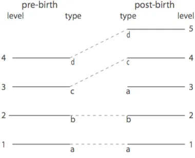
Consider an infinite size population evolving forward in time. LetE=R×N∗. Each(s,i)inEdenotes the (unique) individual living at timesand leveli. This level is affected according to the persistence of each individual: the higher the level is, the faster the individual will die. Let (Ni,j, 0 ≤ i < j) be independent Poisson processes with rate 1. At a jumping time t of Ni j, the individual (t−,i)
reproduces and its unique child appears at level j. At the same time every individual having level at least jis pushed one level up (see Figure 1). These reproduction events involving levelsiand j are called look-down events (as jlooks down ati).
2.1.2 Partition of the set of individuals in lines
We can construct a partition of Ein lines associated to the processes Ni,j as follows. This partition
contains the immortal line ι = R× {1}. All the individuals which belong to the immortal line are called immortal individuals. The other lines of the partition start at look-down events: if an individual is born at level j≥2 at times0 by a look-down event (which means thats0 is a jumping time ofNi,j for somei), it initiates a new line
G= [
k∈N
[sk,sk+1)× {j+k},
of this line. We say that a line is alive at timet if bG≤t<dG, andkis the level ofG at timet if the individual(t,k)∈G. We writeGt for the set of all lines alive at time t. A line at level j is pushed at rate 2j
to level j+1 (since there are 2j
possible independent look-down events which arrive at
rate 1 and which push a line living at level j). SincePj≥21/ j 2
[image:6.612.103.293.170.324.2]
<∞, we get that any line but the immortal one dies in finite time.
Figure 1: A look-down event between levels 1 and 3. Each line living at level at least 3 before the look-down event is pushed one level up after it.
2.1.3 The genealogy
Let (t,j) be an individual in a lineG. An individual(s,i) is an ancestor of the individual (t,j) if
s≤t and either(s,i)∈G, or there is a finite sequence of linesG0,G1,G2, . . . ,Gn=G such that each lineGkis initiated by a child of an individual inGk−1, k=1, 2, . . . ,nand(s,i)∈G0.
For any fixed time t0, we can introduce the following family of equivalence relations R(t0) =
(R(t0)
s ,s ≥ 0): iR
(t0)
s j if the two individuals (t0,i) and (t0,j) have a common ancestor at time
t0−s. It is then easy to show that the coalescent process on N∗ defined byR(t0) is the Kingman’s
coalescent. See Figure 2 for a graphical representation.
2.1.4 Fixation curves
In the study of MRCA, some lines will play a particular role. We say that a lineG is a fixation curve if(bG, 2)∈G: the initial look-down event was from 2 to 1.
Figure 2: The look down process and its associated coalescent tree, started at time t for the 5 first levels. At each look-down event, a new line is born. We indicate at which level this line is at timet. The line of the individual(t, 5)is bold.
joint distribution of(Zt,L0(t),L1(t), . . . ,LZt(t))is given in Theorem 2 of[26], and the distribution ofZt is given in Theorem 3 of[26].
2.1.5 The two oldest families
We consider the partition of the population into the two oldest families given by the equivalence relation Rt(−t)A
t. This corresponds to the partition of individuals alive at time t whose ancestor at time bG
2.1.6 Stationarity and PASTA property
We setHt= (Xt,Yt,Zt,L(t),L1(t), . . . ,LZt(t)). We are interested in the distribution ofHt at as well as the distribution of the labels of the individuals of the same oldest family. By stationarity, those distributions does not depend oftfor fixedt. Arguing as in the proof of Theorem 2 of[26]they are also the same if t is a time when a new MRCA is established. This is the so-called PASTA (Poisson Arrivals See Time Average) property, see[1]for a review on this subject, where the Poisson process considered corresponds to the times when the MRCA changes. For this reason, we shall omit the subscript and writeH, and carry out the proofs at a time when a new MRCA is established.
2.2
Size of the new two oldest families
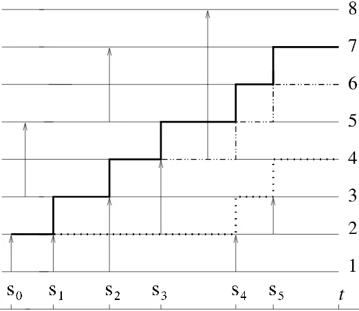
We are interested in the description of the population, and more precisely in the relative size of the two oldest families at the time when a new MRCA is established. Let G∗ be a fixation curve and G be the next fixation curve: they have been initiated by two successive present or future MRCAs. Lets0 = bG∗ be the birth time ofG∗ and(sk,k ∈N
∗) be the jumping times ofG
∗. Notice that s1 = bG corresponds to the birth time of G. Let N ≥ 2. Notice that at time sN−1, only the individuals with level 1 to N will have descendants at the death time dG∗ of G∗. They correspond
to the ancestors at timesN−1 of the population living at time dG∗. We consider the partition into 2
subsets given byR(sN−1)
sN−1−s0 which corresponds to the partition of individuals alive at timesN−1 with
labelsk∈ {1, . . . ,N}whose ancestor at times1is either the individual(s1, 2)which has initiatedGor the immortal individual. We setσN(k) =1 if this ancestor is the immortal individual andσN(k) =0 if it is(s1, 2). LetVN =PNk=1σN(k) be the number of individuals at timesN−1 whose ancestor at times1 is the immortal individual, see Figure 3 for an example. Notice that limN→∞VN/N will be the proportion of the oldest family which contains the immortal individual when(bG∗, 2)becomes
the MRCA of the population. By construction the process(σN,N ∈N∗)is Markov. Notice Theorem 2.1 below gives that(VN,N∈N∗)is also Markov.
In order to give the law of(VN,σN)we first recall some facts on Pólya’s urns, see[19]. LetS(Ni,j)be the number of green balls in an urn afterN drawing, when initially there wasigreen balls and j of some other color in the urn, and where at each drawing, the chosen ball is returned together with one ball of the same color. The process(SN(i,j),N∈N)is a Markov chain, and forℓ∈ {0, . . . ,N}
P
S(Ni,j)=i+ℓ=
N
ℓ
(i+ℓ−1)!(j+N−ℓ−1)!(i+ j−1)!
(i−1)!(j−1)!(i+j+N−1)! ·
In particular, fori=2, j=1 andk∈ {1,N+1}, we have
P(S(2,1)
N =k+1) =
2k
(N+2)(N+1)· (5)
The next Theorem is proved in Section 4.1.
Theorem 2.1. Let N ≥2.
i) The process(1+VN+2,N∈N)is a Pólya’s urn starting at(2, 1). In particular, VN has a size-biased
uniform distribution on{1, . . . ,N−1}, i.e.
P(VN =k) = 2k
Figure 3: In this example, the fixation curveG∗is bold whereas the next fixation curveG is dotted. At times1, we haveσ2= (1, 0)andV2 =1. At times2, we haveσ3 = (1, 0, 1)andV3=2. At time
s3, we haveσ4= (1, 0, 1, 0)andV4=2. At times4, we haveσ5= (1, 1, 0, 1, 0)andV5=3. At time
s5, we haveσ6= (1, 1, 1, 0, 1, 0)andV6=4.
ii) Conditionally on(V1, . . . ,VN),σN is uniformly distributed on the possible configurations: {σ∈ {0, 1}N;σ(1) =1and PNk=1σ(k) =VN}.
Remark2.2. We now give an informal proof of Theorem 2.1-i). If one forgets about the levels of the individuals but for the immortal one, one gets that when there areN lines, the immortal line gives birth to a new line at rateN, whereas one line taken at random (different from the immortal one) gives birth to a new line at rateN/2. Among thoseN−1 lines,VN−1 have a common ancestor with the immortal line at times1, N−VN do not. Let us say the former are of type 1 and the other are
of type 0. The lines of type 0 are increased by 1 at rate(N−VN)N/2. Taking into account that the immortal line gives birth to lines of type 1, we get that the lines of type 1 are increased by 1 at rate
N+ (VN−1)N/2. The probability to add a line of type 1 is then(VN+1)/(N+1). SinceV2=1, we recover that(1+VN,N ≥2)is a Pólya’s urn starting at(2, 1).
Notice that, in general, if N0 ≥ 3, the process (VN0+N,N ∈ N) conditionally on σN0 can not be
described using Pólya’s urns.
Results on Pólya’s urns, see Section 6.3.3 of [19], give that (VN/N,N ∈ N∗) converges a.s. to a random variableY with a beta distribution with parameters(2, 1). This gives the following result.
If one chooses a new oldest family at random (with probability 1/2 the one which contains the im-mortal individual and with probability 1/2 the other one), then its relative proportionX is uniform on (0, 1). This is coherent with the Remark 3.2 given in [26]. Notice that Y has the size biased distribution of X, which corresponds to the fact that the immortal individual is taken at random from the two oldest families with probability proportional to their size.
2.3
Level of the next fixation curve
We keep notations from the previous section. LetL(N)+1 be the level of the fixation curveG when the fixation curveG∗reaches levelN+1, that is at timesN−1. Notice thatL(N)belongs to{1, . . . ,VN}. The law of(L(N),VN)will be useful to give the joint distribution of(Z,Y), see Section 2.5. It also
implies (7) which was already given by Lemma 7.1 of[26]. The process L(N)is an inhomogeneous Markov chain, see Lemma 6.1 of[26]. By construction, the sequence(L(N),N≥2)is non-decreasing and converges a.s. toLdefined in Section 2.1. The next Proposition is proved in Section 4.2.
Proposition 2.4. Let N ≥2.
i) For1≤i≤k≤N−1, we have
P(L(N)=i,VN =k) =2(N−i−1)!
N!
k! (k−i)!
N−k
N−1, (6)
and for all i∈ {1, . . . ,N−1},
P(L(N)=i) = N+1
N−1
2
(i+1)(i+2)· (7)
ii) The sequence((L(N),VN/N),N∈N∗)converges a.s. to a random variable(L,Y), where Y has a
beta(2, 1)distribution and conditionally on Y , L is geometric with parameter1−Y .
A straightforward computation gives that fori∈N∗
P(L=i) = 2 (i+1)(i+2)·
This result was already in Proposition 3.1 of[26].
The level L+1 corresponds to the level of the line of the current MRCA, when the MRCA is newly established. Recall L1(t)is the level at time t of the second fixation curve. We use the convention
L1(t) = 1 if there is only one fixation curve i.e. Z(t) = 0. Just before the random time dG∗ of the death of the fixation curve G∗, we have L1(dG
∗−) = L0(dG∗) = L+1. At a fixed time t, by
stationarity, the distribution of L1(t) does not depend on t, and equation (3.4) from [26] gives that L1(t) is distributed as L. In view of Remark 4.1 in[26], notice the result is also similar for
2.4
Next fixation time
We consider the time dG∗ of death of the lineG∗(which corresponds to a time when a new MRCA
is established). At this time,Y is the proportion of the oldest family which contains the immortal individuals. We denote byτthe time we have to wait for the next fixation time. It is the time needed by the highest fixation curve alive at time dG∗ to reach ∞. Hence, by the look-down construction,
we get that
τ(=d) ∞
X
k=L
2
k(k+1)Ek (8)
where Ek are independent exponential random variables with parameter 1 and independent of Y
andL. See also Theorem 1 in[26].
Proposition 2.5. Let a∈N∗. The distribution of the waiting time for the next fixation time is given by:
forλ∈R+,
E[e−λτ|Y,L=a] = ∞
Y
k=a
k(k+1)
k(k+1) +2λ
. (9)
Its first two moments are given by:
E[τ|Y,L=a] = 2
a and E[τ
2|Y,L=a] =−8
a+8
X
k≥a
1
k2· (10)
We also have: for y,x ∈(0, 1)andλ∈R+,
E[e−λτ|Y = y] = (1−y) ∞
X
ℓ=1
yℓ−1
∞
Y
k=ℓ
k(k+1)
k(k+1) +2λ
, (11)
E[e−λτ|X =x] =x(1−x) ∞
X
ℓ=1
xℓ−1+ (1−x)ℓ−1 ∞
Y
k=ℓ
k(k+1)
k(k+1) +2λ
. (12)
We deduce from (10) thatE[τ|L =a] = 2
a, which was already in Theorem 1 in[26]. Notice that
using (11), we recover the following result.
Corollary 2.6. The random variableτis exponential with mean1.
Using (10) and the fact thatLis geometric with parameter 1−Y, we recover the well known results from Kimura and Ohta[20; 21](see also[12]):
E[τ|Y =y] =−2(1−y)log(1−y)
y , (13)
E[τ2|Y =y] =8 (1−y)log(1− y)
y −
Z 1
y
log(1−z)
z dz
!
. (14)
Lemma 2.7. Let Y be a beta (2,1) random variable and X =ǫY+(1−ǫ)(1−Y)whereǫis independent of Y and such that P(ǫ = 1) = P(ǫ = −1) = 1/2. Then X is uniform on [0, 1]. Furthermore, if W is integrable and independent of ǫ, then we have E[W|X] = X g(X) + (1−X)g(1−X) where g(y) =E[W|Y = y].
We also get, thanks to the above Lemma that:
E[τ|X =x] =−2 xlog(x) + (1−x)log(1−x)
, and (15)
E[τ2|X =x] =8 xlog(x) + (1−x)log(1−x)−x
Z 1
x
log(1−z)
z dz (16)
−(1−x)
Z 1
1−x
log(1−z)
z dz
!
.
2.5
Number of individuals present which will become MRCA
We keep notations from Sections 2.1 and 2.3. We set Z = ZdG∗ the number of individuals living
at time dG∗ which will become MRCA of the population in the future. Let L0 = L(dG∗) +1 and (L0,L1, . . . ,LZ) = (L0(dG∗), . . . ,LZ(dG∗))be the levels of the fixation curves at the death time ofG∗. Recall notations from Section 2.2. The following Lemma and Proposition 2.4 characterize the joint distribution of(Y,Z,L,L1, . . . ,LZ).
Lemma 2.8. Conditionally on(L,Y)the distribution of(Z,L1, . . . ,LZ)does not depend on Y . Condi-tionally on{L=N},(Z,L1, . . . ,LZ)is distributed as follows:
1. Z=0if N=1;
2. Conditionally on{Z≥1}, L1 is distributed as L(N)+1.
3. For N′∈ {1, . . . ,N−1}, conditionally on{Z≥1,L1=N′+1},(Z−1,L2, . . . ,LZ)is distributed
as(Z,L1, . . . ,LZ)conditionally on{L=N′}.
Remark 2.9. If one is interested only in the distribution of (Z,L0, . . . ,LZ,L), one gets that {LZ, . . . ,L0} is distributed as {k;Bk = 1} where (Bn,n ≥ 2) are independent Bernoulli r.v. such
thatP(Bk=1) =1/ k 2
. In particular we have
Z(=d)X
k≥2
Bk−1. (17)
Indeed, set Bk = 1 if the individual (k,dG∗) at level k belongs to a fixation curve and Bk = 0 otherwise. Notice that Bk = 1 if none of the k−2 look-down events which pushed the line of (k,dG∗)between its birth time anddG∗ involved the line of(k,dG∗). This happens with probability
P(Bk=1) =
k−1 2
k
2
· · ·
2 2
3 2
=
1
k
2
.
Moreover Bk is independent of B2, . . . ,Bk−1 which depends on the lines below the line of (k,dG∗)
sup{k;Bk = 1} −1. We deduce that conditionally on L = a, Z = Pak=2Bk (with the convention
Z=0 ifa=1). In particular, we get
E[(1+λ)Z|L=a] =
a
Y
k=2
E[(1+λ)Bk] =
a
Y
k=2
k(k−1) +2λ
k(k−1) =
a−1
Y
k=1
k(k+1) +2λ
k(k+1) .
The result does not change if one considers a fixed timet instead ofdG∗.
We deduce the following Corollary from the previous Remark and Lemma 2.8 and for the first two moments (20) we use (10) and Proposition 1.3.
Corollary 2.10. Let a ≥ 1. Conditionally on (Y,L), Z (=d)
L
X
k=2
Bk (with the convention
P
; = 0),
where (Bk,k ≥ 2) are independent Bernoulli random variables independent of (Y,L) and such that
P(Bk=1) =1/ k 2
. We have for allλ≥0,
E[(1+λ)Z|Y,L=a] =
a−1
Y
k=1
k(k+1) +2λ
k(k+1) , (18)
with the conventionQ;=1. We haveP(Z=0|Y,L=1) =1and for k≥1,
P(Z=k|Y,L=a) = 2
k−1
3
a+1
a−1
X
1<ak<···<a2<a
k
Y
i=2
1
(ai−1)(ai+2)· (19)
We also have
E[Z|Y,L=a] =2−2
a and E[Z
2|Y,L=a] =18−4π 2
3 − 18
a +8
X
k≥a
1
k2· (20)
We are now able to give the distribution of Z conditionally on Y or X. We deduce from ii) of Proposition 2.4 and from Corollary 2.10 the next result.
Corollary 2.11. Let y∈[0, 1]. We have, for allλ≥0,
E[(1+λ)Z|Y= y] = (1−y) +∞
X
a=1
ya−1
a−1
Y
k=1
k(k+1) +2λ
k(k+1) , (21)
with the conventionQ;=1. We haveP(Z=0|Y = y) =1−y, and, for all k∈N∗,
P(Z=k|Y = y) = 2
k−1
3 (1−y)
X
1<ak<···<a1<∞
(a1+1)(a1+2)ya1−1
k
Y
i=1
1 (ai−1)(ai+2)
. (22)
We also have
E[Z|Y = y] =2
1+1−y
y log(1−y)
Corollary 2.12. Let x∈[0, 1]. We have, for allλ≥0,
E[(1+λ)Z|X =x] =x(1−x) ∞
X
a=2
xa−1+ (1−x)a−1 +∞
X
a=1
a−1
Y
k=1
k(k+1) +2λ
k(k+1) , (24)
with the conventionQ;=1. We haveP(Z=0|X =x) =2x(1−x), and, for all k∈N∗,
P(Z=k|X =x)
= 2
k−1
3 x(1−x)
X
1<ak<···<a1<∞
(a1+1)(a1+2)
xa1−2+ (1−x)a1−2
k
Y
i=1
1
(ai−1)(ai+2)· (25)
We also have
E[Z|X =x] =2 1+xlog(x) + (1−x)log(1−x)
. (26)
The second moment of Z conditionally on Y (resp. X) can be deduced from (21) (resp. (24)) or from (4) and (14) (resp. (16)).
Some elementary computations give:
P(Z=0|X =x) =2x(1−x),
P(Z=1|X =x) = 1 3
x2+ (1−x)2−2x(1−x)ln(x(1−x)),
P(Z=2|X =x) = 2 3
11
6(x
2+ (1−x)2)−(1−x)ln(1−x)−xln(x)
+2
3x(1−x)
2− π 2
3 +2 ln(x)ln(1−x)− 1
3ln(x(1−x))
.
We recover by integration of the previous equations the following results from[26]:
P(Z=0) = 1
3, P(Z=1) = 11
27 and P(Z=2) = 107 243−
2 81π
2.
3
Stationary distribution of the relative size for the two oldest families
3.1
Resurrected process and quasi-stationary distribution
Let E be a subset ofR. We recall that if U = (Ut,t ≥ 0) is an E-valued diffusion with absorbing states∆, we say that a distributionν is a quasi-stationary distribution (QSD) of U if for any Borel setA⊂R,
Pν(Ut∈A|Ut6∈∆) =ν(A) t≥0,
where we writePν when the distribution ofU0isν. See also[31]for QSD for diffusions with killing.
Let µand ν be two distributions on E\∆. We define Uµ the resurrected process associated to U, with resurrection distributionµ, underPν as follows:
1. U0is distributed according toν andU µ
2. Conditionally on(τ1,{τ1 < ∞},(Utµ,t ∈[0,τ1))), (Utµ+τ
1,t ≥0)is distributed as U
µ under
Pµ.
According to Lemma 2.1 of [4], the distribution µ is a QSD of U if and only if µ is a stationary distribution ofUµ. See also the pioneer work of[13]in a discrete setting.
The uniqueness of quasi-stationary distributions is an open question in general. We will give a ge-nealogical representation of the QSD for the Wright-Fisher diffusion and the Wright-Fisher diffusion conditioned not to hit 0, as well as for the Moran model for the discrete case.
We also recall that the so-called Yaglom limitµis defined by
lim
t→∞Px(Ut∈A|Ut 6∈∆) =µ(A) ∀A∈ B(R), provided the limit exists and is independent ofx ∈E\∆.
3.2
The resurrected Wright-Fisher diffusion
From Corollary 2.3 and comments below it, we get that the relative proportion of one of the two oldest families at a time when a new MRCA is established is distributed according to the uniform distribution over [0, 1]. Then the relative proportion evolves according to a Wright-Fisher (WF) diffusion. In particular it hits the absorbing state of the WF diffusion,{0, 1}, in finite time. At this time one of the two oldest families dies out and there a new MRCA is (again) established.
The QSD distribution of the WF diffusion exists and is the uniform distribution, see[12, p. 161], or [18]for an explicit computation. From Section 3.1, we get that in stationary regime, for fixed
t (and of course at time when a new MRCA is established) the relative size, Xt, of one of the two oldest families taken at random is uniform over(0, 1).
Similar arguments as those developed in the proof of Proposition 3.1 yield that the uniform distri-bution is the only QSD of the WF diffusion. Lemma 2.1 in[4]implies there is no other resurrection distribution which is also the stationary distribution of the resurrected process.
3.3
The oldest family with the immortal line of descent
Recall thatY = (Yt,t∈R)is the process of relative size for the oldest family containing the immortal
individual. From Corollary 2.3, we get that, at a time when a new MRCA is established, Y is distributed according to the beta (2, 1) distribution. Then Y evolves according to a WF diffusion conditioned not to hit 0; its generator is given byL = 1
2 x(1−x)∂ 2
x+(1−x)∂x, see[9; 18]. Therefore
Y is a resurrected Wright-Fisher diffusion conditioned not to hit 0, with beta (2, 1) resurrection distribution.
The Yaglom distribution of the Wright-Fisher diffusion conditioned not to hit 0 exists and is the beta (2, 1)distribution, see[18]for an explicit computation. In fact the Yaglom distribution is the only QSD according to the next proposition.
Proposition 3.1. The only quasi-stationary distribution of the Wright-Fisher diffusion conditioned not to hit0is the beta(2, 1)distribution.
Lemma 2.1 in[4]implies that the beta(2, 1)distribution is therefore the stationary distribution of
Y. Furthermore, the resurrected Wright-Fisher diffusion conditioned not to hit 0, with resurrection
3.4
Resurrected process in the Moran model
The Moran model has been introduced in[25]. This mathematical model represents the neutral evolution of a haploid population of fixed size, say N. Each individual gives, at rate 1, birth to a child, which replaces an individual taken at random among theNindividuals. Notice the population size is constant. Letξt denote the size of the descendants at time t of a given initial group. The process ξ= (ξt,t ≥ 0) goes from state k to state k+ǫ, where ǫ ∈ {−1, 1}, at rate k(N−k)/N. Notice that 0 and N are absorbing states. They correspond respectively to the extinction of the descendants of the initial group or its fixation. The Yaglom distribution of the processξis uniform over{1, . . . ,N−1}(see[12, p. 106]). Since the state is finite, the Yaglom distribution is the only QSD.
Let µ be a distribution on {1, . . . ,N−1}. We consider the resurrected process (ξµt,t ≥ 0) with resurrection distributionµ. The resurrected process has the same evolution asξuntil it reaches 0 orN, and it immediately jumps according toµwhen it hits 0 orN. The processξµ is a continuous time Markov process on{1, . . . ,N−1}with transition rates matrixΛµgiven by:
Λµ(1,k) =µ(k) +1{k=2}
N−1
N fork∈ {2, . . . ,N−1},
Λµ(k,k+ǫ) = k(N−k)
N forǫ∈ {−1, 1}andk∈ {2, . . . ,N−2},
Λµ(N−1,k) =µ(k) +1{k=N−2}
N−1
N fork∈ {1, . . . ,N−2}.
We deduce from[13], thatµis a stationary distribution for ξµ (i.e. µΛµ=0) if and only ifµis a QSD forξ, hence if and only ifµis uniform over{1, . . . ,N−1}.
Using the genealogy of the Moran model, we can give a natural representation of the resurrected processξµ when the resurrection distribution is the Yaglom distribution. Since the genealogy of the Moran model can be described by the restriction of the look-down process toE(N)=R× {1, . . . ,N}, we get from Theorem 2.1 that the size of the oldest family which contains the immortal individual is distributed as the size-biased uniform distribution on{1, . . . ,N−1}at a time when a new MRCA is established. The PASTA property also implies that this is the stationary distribution. If, at a time when a new MRCA is established, we consider at random one of the two oldest families (with probability 1/2 the one with the immortal individual and with probability 1/2 the other one), then the size process is distributed as(ξµt,t ∈R) under its stationary distribution, with µ the uniform distribution.
Remark 3.2. We can also consider the Wright-Fisher model (see e.g. [9]) in discrete time with a population of fixed finite sizeN,ζ= (ζk,k∈N). This is a Markov chain with state space{0, . . . ,N} and transition probabilities
P(i,j) =
N
j i N
j
1− i
N
N−j
.
There exists a unique quasi-stationary distribution,µN (which is not the uniform distribution), see
4
Proofs
4.1
Proof of Theorem 2.1
We consider the set
AN =
(k1, . . . ,kN);k1=1, fori∈ {1, . . . ,N−1},ki+1∈
ki,ki+1
.
Notice thatP(V1 =k1, . . . ,VN = kN)>0 if and only if (k1, . . . ,kN)∈AN. To prove the first part of Theorem 2.1, it is enough to show that, forN ≥2 and(k1, . . . ,kN+1)∈AN+1,
P(VN+1=kN+1|VN=kN, . . . ,V1=k1) =
(
1−1+kN
N+1 if kN+1=kN, 1+kN
N+1 if kN+1=1+kN.
(27)
ForpandqinN∗such thatq<p, we introduce the set:
∆p,q={α= (α1, . . . ,αp)∈ {0, 1}p,α1=1,
p
X
i=1
αi =q}.
Notice that Card(∆p,q) = p−1
q−1
. Hence to prove the second part of Theorem 2.1, it is enough to show that: for all(k1, . . . ,kN)∈AN, and allα∈∆N,kN,
P(σN=α|VN=kN, . . . ,V1=k1) = 1
N−1
kN−1
· (28)
We proceed by induction on N for the proof of (27) and (28). The result is obvious forN =2. We suppose that (27) and (28) are true for a fixedN. We denote byINandJN, 1≤IN <JN≤N+1, the two levels involved in the look-down event at timesN. Notice that(IN,JN)andσN are independent. This pair is chosen uniformly so that, for 1≤i< j≤N+1,
P(IN=i,JN = j) = 2 (N+1)N,
P(IN=i) = 2(N−i+1) (N+1)N ,
P(JN =j) = 2(j−1) (N+1)N·
For α = α1, . . . ,αN+1
∈ {0, 1}N+1 and j ∈ {1, . . . ,N + 1}, we set α×j = α1, . . . ,αj−1, αj+1, . . . ,αN+1
∈ {0, 1}N.
Let us fix(k1, . . . ,kN+1)∈AN+1, andα= α1, . . . ,αN+1
∈∆N+1,kN+1. Notice that {σN+1 =α} ⊂
{VN+1=kN+1}. We first compute
1st case: kN+1=kN+1.We have:
P(σN+1=α|VN =kN, . . . ,V1=k1)
= X
1≤i<j≤N+1
P(IN=i,JN = j,σN+1=α|VN=kN, . . . ,V1=k1)
= X
1≤i<j≤N+1,αi=αj=1
P(IN=i,JN = j,σN=α×j|VN =kN, . . . ,V1=k1)
= X
1≤i<j≤N+1,αi=αj=1
P(IN=i,JN = j)P(σN =αj
×|VN=kN, . . . ,V1=k1)
= X
1≤i<j≤N+1,αi=αj=1 2 (N+1)N
1
N−1
kN−1
= 2 (N+1)N
1
N−1
kN−1
kN+1(kN+1−1) 2
=(kN+1)!(N−kN)!
(N+1)! , (29)
where we used the independence of(IN,JN)andσN for the third equality, the uniform distribution ofσN conditionally onVN for the fourth, and thatkN+1=kN+1 for the sixth. Hence, we get
P(VN+1=kN+1|VN =kN, . . . ,V1=k1) =
X
α∈∆N+1,kN+1
P(σN+1=α|VN=kN, . . . ,V1=k1)
=
N
kN+1−1
(k
N+1)!(N−kN)!
(N+1)!
=1+kN
N+1· (30)
2nd case: kN+1=kN.Similarly, we have:
P(σN+1=α|VN=kN, . . . ,V1=k1) =
X
1≤i<j≤N+1,αi=αj=0 2 (N+1)N
1
N−1
kN−1
= 2
(N+1)N
1
N−1
kN−1
(N+1−kN)(N−kN)
2
= (N−kN)(kN−1)!(N−kN+1)!
(N+1)! . (31)
Hence, we get
P(VN+1=kN|VN=kN, . . . ,V1=k1) =
X
α∈∆N+1,kN+1
P(σN+1=α|VN=kN, . . . ,V1=k1)
=
N
kN+1−1
(N−k
N)(kN−1)!(N−kN+1)!
(N+1)!
=1−1+kN
Equalities (30) and (32) imply (27). Moreover, we deduce from (29) and (31) that, for kN+1 ∈ {kN,kN+1},
P(σN+1=α|VN+1=kN+1, . . . ,V1=k1) =
P(σN+1=α,VN+1=kN+1|VN=kN, . . . ,V1=k1) P(VN+1=kN+1|VN =kN, . . . ,V1=k1)
= 1N
kN+1−1
,
which proves that (28) withN replaced byN+1 holds. This ends the proof.
4.2
Proof of Proposition 2.4
Theorem 2.1 shows that the distribution ofσN conditionally onVN is uniform. Then, ifVN =k, we can see L(N)as the number of draws (without replacement) we have to do in a two-colored urn of size N−1 with k−1 black balls until we obtain a white ball. Hence, fork ∈ {1, . . . ,N−1}and
i∈ {1, . . . ,k},
P(L(N)=i|VN=k) = k−1
N−1
k−2
N−2· · ·
k−i+1
N−i+1
N−k N−i
= (N−i−1)! (N−1)!
(k−1)!
(k−i)!(N−k).
This and Theorem 2.1 give (6).
It is easy to prove by induction on jthat for all j∈N,
i+j
X
k=i
k! (k−i)!=
(i+j+1)!
j!(i+1) · (33)
Summing (6) overk∈ {i, . . . ,N−1}gives:
P(L(N)=i) = 2(N−i−1)!
N!(N−1)
N−1
X
k=i
k!
(k−i)!(N−k)
= 2(N−i−1)!
N!(N−1)
(N+1)
N−1
X
k=i
k! (k−i)!−
N−1
X
k=i
(k+1)! ((k+1)−(i+1))!
= 2(N−i−1)!
N!(N−1)
(N+1)!
(N−i−1)!(i+1)−
(N+1)! (N−i−1)!(i+2)
=2N+1
N−1
1 (i+1)(i+2),
Since (L(N),n ∈ N∗) is non-decreasing, we deduce from Theorem 2.1 that the sequence ((L(N),V(N)/N),N∈N∗)converges a.s. to a limit(L,Y). Leti≥1 andv∈[0, 1). We have:
P
L(N)=i,VN
N ≤v
= ⌊N v⌋
X
k=i
PL(N)=i,VN=k
= ⌊N v⌋
X
k=i
2(N−i−1)!
N!
k! (k−i)!
N−k N−1
= 2
N
⌊N v⌋
X
k=i
k N−1
k−1
N−2· · ·
k−i+1
N−i
1− k−1
N−1
,
which converges to 2
Z v
0
yi(1− y)d y as N goes to infinity. We deduce that P(L = i,Y ≤ v) =
2Rv 0 y
i(1−y)d y fori∈N∗and v∈[0, 1). Thus Y has a beta(2, 1) distribution and conditionally onY, Lis geometric with parameter 1−Y.
4.3
Proof of Proposition 2.5
The Laplace transform (9) comes from (8). We deduce from (8) that
E[τ|Y,L=a] =X
k≥a
2
k(k+1)= 2
a,
and that
E[τ2|Y,L=a] =8
X
k≥a
1
k(k+1)
X
ℓ≥k
1 ℓ(ℓ+1)
=8X
k≥a
1
k2(k+1)
=8X
k≥a
1
k2 −8
X
k≥a
1
k(k+1)
=8X
k≥a
1
k2 −
8
a·
4.4
Proof of Corollary 2.6
We give a direct proof. We set ck = k(k+1) and bk = ck−2 = (k−1)(k+2). Notice that
ck+2λ= bk+2(1+λ). We have from (11)
E[e−λτ] =
Z 1
0
2y d y X
a≥1
(1− y)ya−1Y
k≥a
ck
ck+2λ
!
=2X
a≥1
1 (a+1)(a+2)
Y
k≥a
ck
ck+2λ
=2X
a≥1
1
ba+2(λ+1)
Y
k≥a+1
bk bk+2(1+λ)
= 1
1+λNlim→+∞
N
X
a=1
1− ba
ba+2(1+λ)
Y
k≥a+1
bk bk+2(1+λ)
= 1
1+λNlim→+∞
Y
k≥N+1
bk
bk+2(1+λ)
= 1 1+λ,
where for the last equality we used that limN→∞Qk≥N+1 bk
bk+2(1+λ) =1.
4.5
Proof of Lemma 2.8
Let us fixN≥2. We have introduced L(N)+1 as the level of the fixation curveG when the fixation curve G∗ reaches level N+1, that is at timesN−1. We denote by ZN the number of other fixation curves alive at this time, andL(1N)>L2(N)>· · ·> L(ZN)
N =2 their levels. By construction of the fixation curves, the result given by Lemma 2.8 is straightforward for(VN/N,ZN,L(N),L1(N),L(2N), . . . ,L(ZN)
N ) in-stead of (Y,Z,L,L1, . . . ,LZ). Now, using similar arguments as for the proof of the second part
of Proposition 2.4, we get that (VN/N,ZN,L(N),L
(N) 1 ,L
(N) 2 , . . . ,L
(N)
ZN ),N ≥ 2
converges a.s. to (Y,Z,L,L1, . . . ,LZ)which ends the proof.
4.6
Proof of Lemma 1.1
Only the second part of this Lemma has to be proved. Assumetis either fixed or a time when a new MRCA is established. The fact that the coalescent timesAt(and thus the TMRCA ) does not depend on the coalescent tree shape can be deduced from[33], Section 3, see also [6]. In particular, At
does not depend on(Xt,Yt,Lt,Zt)neither onτt which conditionally on the past depends only on the coalescent tree shape (see Section 2.4).
4.7
Proof of Theorem 1.2
The distribution ofY is given by Corollary 2.3. Properties ii) and vii) are straightforward by con-struction of X. Proposition 2.4 implies iii). Proposition 2.5 implies iv) and Corollary 2.10 implies v). We deduce vi) from (8), as the exponential random variables are independent of the past before
dG∗.
4.8
Proof of Proposition 3.1
Letµ1be the beta(2, 1)distribution. Using[4], it is enough to prove thatµ1 is the only probability distributionµon[0, 1)such thatµis invariant forYµ. Sincex 7→Ex[τ]is bounded (see (15)), we get thatEµ[τ]<∞. For a measureµand a function f, we set〈µ,f〉=R f dµwhen this is well de-fined. AsEµ[τ]<∞, it is straightforward to deduce from standard results on Markov chains having one atom with finite mean return time (see e.g. [23]for discrete time Markov chains) thatYµ has
a unique invariant probability measureπ which is defined by〈π,f〉 =Eµ
Z τ
0
f(Ys)ds
/Eµ[τ].
Hence we have
Eµ
Zτ
0
f(Ys)ds
=〈π,f〉Eµ[τ]. (34)
Letτn be the n-th resurrection time (i.e. n-th hitting time of 1) after 0 of the resurrected process
Yµ: τ1 =τand forn∈N∗, τn+1 =inf{t > τn;Ytµ−=1}. The strong law of large numbers implies that for any real measurable bounded function f on[0, 1),
Pµ−a.s. 1
τn
Z τn
0
f(Ys)ds −−−→
n→∞ 〈π,f〉.
RecallL is the infinitesimal generator ofY. For g any C2 function defined on [0, 1], the process
Mt=g(Yt)−
Z t
0
Lg(Ys)dsis a martingale. Since|Mt| ≤ kgk∞+t(kg′k∞+kg′′k∞)andEµ[τ]<∞,
we can apply the optional stopping theorem for(Mt,t≥0)at timeτto get that
g(1)−Eµ
Z τ
0
Lg(Ys)ds
=〈µ,g〉·
If aC2 functiongλ is an eigenvector with eigenvalue−λ(withλ >0) such that gλ(1) =0, we de-duce from (34) that〈µ,gλ〉=λEµ[τ]〈π,gλ〉. Therefore, if the resurrection measure is the invariant measure, we get:
〈µ,gλ〉=λEµ[τ]〈µ,gλ〉. (35)
Let(aλn,n≥0)be defined byaλ0 =1 and, forn≥0,
aλn+1= n(n+1)−2λ (n+1)(n+2)a
λ
n.
The functionP∞n=0aλnxn solves Lf =−λf on [0, 1). For N ∈N∗ andλ= N(N+1)
2 , notice that
f). Notice that P1(x) =1−x, which implies that〈µ,P1〉>0. We deduce from (35) thatEµ[τ] =1 and〈µ,PN〉 = 0 for N ≥2. As PN(1) =0 for all N ≥ 1, we can write PN(x) = (1−x)QN−1(x), where QN−1 is a polynomial function of degree N−1. For the probability distribution ¯µ(d x) =
1−x
〈µ,P1〉µ(d x), as
〈µ,PN+1〉
〈µ,P1〉
=0, we get that:
〈µ¯,QN〉=0, for allN≥1. (36)
Since ¯µis a probability distribution on[0, 1], it is characterized by (36). To conclude, we just have to check that ¯µ1 satisfies (36). In fact, we shall check that 〈µ1,gλ〉 = 0 for any C2 function gλ eigenvector ofL with eigenvalue−λsuch thatgλ(1) =0 andλ6=1. Indeed, we have
−λ〈µ1,gλ〉=−λ
Z 1
0
2x gλ(x)d x
=
Z 1 <