AN EIGENVALUE INEQUALITY AND SPECTRUM LOCALIZATION
FOR COMPLEX MATRICES∗
MARIA ADAM† AND MICHAEL J. TSATSOMEROS‡
Abstract. Using the notions of the numerical range, Schur complement and unitary equivalence,
an eigenvalue inequality is obtained for a general complex matrix, giving rise to a region in the complex plane that contains its spectrum. This region is determined by a curve, generalizing and improving classical eigenvalue bounds obtained by the Hermitian and skew-Hermitian parts, as well as the numerical range of a matrix.
Key words. Eigenvalues, Inclusion regions, Numerical range, Hermitian part.
AMS subject classifications. 15A18, 15A60.
1. Introduction. In this article, we consider complex matrices A ∈ Mn(C),
n ≥ 2, and obtain an inequality satisfied by the real and imaginary part of every eigenvalue of A (Section 3).In turn, this inequality gives rise to a region in the complex plane that contains the spectrum of A (Section 4).We examine when an eigenvalue lies on the boundary of such a region.The proof of the main inequality in Theorem 3.1 is an adaptation to general matrices of the proof of [7, Theorem 3.1] for almost skew-symmetric matrices.As a consequence, the spectrum localization results for almost skew-symmetric matrices and (hyper)tournaments obtained in [2, 3, 6, 7] follow as special cases.Furthermore, the fact that Theorem 3.1 holds for general matrices allows its application to rotationseiθA, giving rise to improved localization
results for the spectrum.Our concluding remarks outline some related research goals (Section 5).
2. Notation and preliminaries. We begin by settling on the notation to be used.For A ∈ Mn(C), its spectrum is denoted by σ(A) and its spectral radius by
ρ(A) = max{|λ|:λ ∈σ(A)}.We writeA=H(A) +S(A), where
H(A) = A+A
∗
2 and S(A) =
A−A∗
2
are theHermitian partand theskew-Hermitian partofA, respectively.Thenumerical rangeis the set
F(A) = {v∗Av∈C:v∈Cn withv∗v= 1},
which is a compact and convex subset ofCthat contains the spectrum ofA(see [5]). Recall that A is Hermitian if and only if F(A) ⊂R, and that if A is normal, then
∗Received by the editors 9 December 2005. Accepted for publication 28 August 2006. Handling
Editor: Raphael Lowey. Research supported by a grant of the EPEAEK project Pythagoras II. The project is co-funded by the European Social Fund (75%) and Greek National Resources (25%).
†Department of Mathematics, National Technical University of Athens, Athens 15780, Greece
‡Mathematics Department, Washington State University, Pullman, WA 99164-3113, U.S.A.
F(A) coincides with the convex hull ofσ(A).It is also well known that
ReF(A) = F(H(A)) and iImF(A) = F(S(A)).
WhenA∈ Mn(R), then F(A) is symmetric with respect to the real axis.Also, any
eigenvalueλ ∈ σ(A) that belongs to the boundary of the numerical range, ∂F(A), is anormal eigenvalue ofA; namely, there exists a unitary matrixU ∈ Mn(C) such
that
U∗AU = λ I
k⊕B,
wherek is the algebraic multiplicity ofλ andλ ∈σ(B); see [5, Theorem 1.6.6]. Given A ∈ Mn(C), let y1 be a unit eigenvector corresponding to the largest eigenvalueδ1of its Hermitian partH(A).We define two quantities to be used in the sequel:
v(A) = S(A)y122 and u(A) = Im(y1∗S(A)y1). (2.1)
Notice that u(A) = 0 when A is real.Also if v(A) = 0, then (δ1, y1) is an eigenpair for bothAand A∗.That is, v(A) can be thought of as a measure of how closeδ1 is
to being a normal eigenvalue ofA.
3. The main eigenvalue inequality. Consider a matrixA ∈ Mn(C) and let
δ1be the largest eigenvalue of its Hermitian partH(A).It is well known that all the eigenvalues ofA lie in the closed half-plane{z ∈C: Rez ≤δ1}.In this section, we obtain a new localization ofσ(A) by replacing the line Rez=δ1with an appropriate curve.We proceed immediately with the inequality satisfied by every eigenvalue of
A∈ Mn(C).
Theorem 3.1. LetA∈ Mn(C)and letλ be an eigenvalue ofA. Let alsoδ1 ≥ δ2
be the two largest eigenvalues of the Hermitian part of A. Then
(Reλ −δ2) (Im λ−u(A))2 ≤ (3.1)
(δ1−Reλ) v(A)−u(A)2+ (Reλ−δ2) (Reλ−δ1).
Proof.Lety1∈Cn be a unit eigenvector ofH(A) corresponding to the eigenvalue
δ1.Then, there exists a unitary U ∈ Mn(C), whose first column isy1, such that
U∗H(A)U =
δ1 0 0 H1
, where H1 = diag(δ2, δ3, . . . , δn), δj∈σ(H(A)).
Moreover, asU∗S(A)U is skew-Hermitian, we have
U∗S(A)U =
iα u∗
−u S1
,
(3.2)
where S1∈ Mn−1(C) is skew-Hermitian,u∈Cn−
1 andα∈R.Consequently, when
λ ∈σ(A),
U∗(A−λ I)U =
δ1+iα−λ u∗ −u H1+S1−λ I
is a singular matrix.Note that by assumption,
iα=y∗
1S(A)y1, i.e., α= u(A). (3.3)
At this stage, consider the case where
λ = δ1+iα = y∗1(H(A) +S(A))y1 = y∗1Ay1;
otherwise (3.1) holds trivially andλ =δ1+iu(A) is a normal eigenvalue ofAon the boundary of the numerical rangeF(A).Then the Schur complement of the leading entry inU∗(A−λ I)U is
E = (H1+S1−λ I) + 1
δ1+iα−λ
uu∗,
which must be singular sinceA−λI is singular [4, p.21]. The Hermitian and skew-Hermitian parts ofE can be readily computed to be
H(E) = H1−Reλ I+
δ1−Reλ
(δ1−Reλ)2+ (α−Imλ)2
uu∗,
(3.4)
and
S(E) = S1−iImλ I+
i(Imλ −α) (δ1−Reλ)2+ (α−Imλ)2
uu∗.
(3.5)
Since 0∈σ(E)⊆F(E) andF(H(E)) = ReF(E) (see [5, Properties 1.2.5, 1.2.6]), it follows that 0∈F(H(E)), which in turn implies that there exists unit x∈Cn such
thatx∗H(E)x= 0; that is,
0 = x∗H1x−x∗xReλ + δ1−Reλ
(δ1−Reλ)2+ (α−Imλ)2
x∗uu∗x, x∗x= 1.
(3.6)
Notice that sinceF(H1) = [δn, δ2] and sinceF(uu∗) = [0, u∗u], we respectively have
that
x∗H
1x ≤ δ2 and x∗uu∗x ≤ u∗u.
Hence from (3.6) we obtain
0 ≤ δ2−Reλ +
δ1−Reλ
(δ1−Reλ)2+ (α−Imλ)2
u∗u.
(3.7)
Denoting by e1 the first standard basis vector in Cn, and since unitary matrices preserve the Euclidean norm, it follows that
α2+u∗u= iα −u 2 2 = U
iα u∗
−u S1
e1 2 2 = U
iα u∗
−u S1
U∗U e
1 2 2
= S(A)y1 2
Equality (3.8) implies that
u∗u= v(A)−α2.
(3.9)
The validity of (3.1) now follows from (3.3), (3.7) and (3.9).
Corollary 3.2. Let A∈ Mn(C)and let δ1> δ2 be the two largest eigenvalues
of the Hermitian partH(A). If 4(v(A)−u(A)2)<(δ
1−δ2)2, then for everyλ ∈σ(A)
with Reλ > δ2, we have thatReλ ∈ (s, t), where
s= δ1+δ2−
(δ1−δ2)2−4(v(A)−u(A)2)
2 ,
t= δ1+δ2+
(δ1−δ2)2−4(v(A)−u(A)2)
2 .
Proof. Considerλ ∈σ(A) such thatδ2<Reλ < δ1.Then by (3.1),
(δ1−Reλ)
v(A)−u(A)2 Reλ−δ2
+ Reλ−δ1
≥ 0.
The latter inequality and the assumption (v(A)−u(A)2)<(δ
1−δ2)2/4 imply directly that either
Reλ ≤ δ1+δ2−
(δ1−δ2)2−4(v(A)−u(A)2) 2
or
Reλ ≥ δ1+δ2+
(δ1−δ2)2−4(v(A)−u(A)2)
2 .
4. Localization of the spectrum. We will use our results in the previous section to obtain an inclusion region for σ(A) determined by a curve Γ(A).This curve comprises the pointss+it∈Cthat satisfy (3.1) as an equality.
In order to define and plot Γ(A), as well as study its position relative to the eigenvalues, it is useful to first rewrite inequality (3.1) by separating the imaginary part from the real part ofλ.
Recalling the proof and notation used in Theorem 3.1, notice that (3.1) takes a trivial form when Reλ=δ1 or Reλ≤δ2.Therefore, let us consider λ ∈σ(A) with
δ2<Reλ < δ1.Then (3.1) implies that
(Imλ −u(A))2
≤ (δ1−Reλ)
v(A)
−u(A)2 Reλ −δ2
+ Reλ−δ1
.
(4.1)
Definition 4.1. Prompted by the latter inequality, we define a curve Γ(A) in
the complex plane associated with the matrixA∈ Mn(C) given by
s+it∈C:s, t∈Rand (t−u(A))2= (δ1−s)
v(A)
−u(A)2
s−δ2
+s−δ1
Recalling the notation and definitions in (2.1), by Cauchy-Schwarz, we have
|y∗
1S(A)y1| ≤ S(A)y12y12.
As y12= 1, the following implications ensue:
Re2(y∗
1S(A)y1) + Im 2
(y∗
1S(A)y1) =|y1∗S(A)y1|2 ≤ S(A)y122= v(A) =⇒
Im2(y∗
1S(A)y1)≤v(A)−Re 2(y∗
1S(A)y1)≤v(A) =⇒
u(A)2
≤v(A).
(4.2)
We can now make the following observations regarding Γ(A).
Observation 4.2.
1.Ifδ1=δ2, the defining equation of Γ(A) becomes
(t−u(A))2+ (s
−δ1)2=
−v(A) + u(A)2= 0;
that is, by (4.2), Γ(A) is degenerate, consisting of only one point.Henceforth we assume thatδ1> δ2.
2.The line{z∈C: Rez=δ2}is a vertical asymptote of Γ(A).
3.Γ(A) is symmetric with respect to the horizontal line {z∈C: Imz= u(A)} which it intercepts atδ1.
4.As the defining equation of Γ(A) for any fixedtis a cubic equation ins, Γ(A) may intercept the line L ={z ∈ C : Imz = u(A)} in up to three distinct points.Specifically, the defining equation of Γ(A) fort= u(A), s=δ2,is
(δ1−s)s2−(δ1+δ2)s+δ1δ2+ v(A)−u(A)2= 0. (4.3)
Consider then the discriminant of the quadratic factor
∆ = (δ1−δ2)2−4v(A)−u(A)2.
◮ If ∆ < 0, then (4.3) has only one real root, δ1.Consequently, Γ(A)
intercepts L only once, at the point (δ1,u(A)) and Γ(A) is a simple open curve; see Examples 4.3 and 4.4.
◮ If ∆>0, then (4.3) has distinct roots
s1=
δ1+δ2− √
∆
2 , s2=
δ1+δ2+ √
∆
In this case Γ(A) comprises two branches one of which is a Jordan curve (closed and simple); see the matrix A in Example 4.5. Note that s1, s2 coincide with the endpoints of the interval (s, t) in Corollary 3.2.
◮ If ∆ = 0, then (4.3) has a double root δ1+δ2
2 and a simple rootδ1.In this case Γ(A) is a folium of Descartes; see the matrixB in Example 4.5.
5.By (4.2) and since for pointss+it∈Γ(A) we have
(δ1−s)
v(A)−u(A)2
s−δ2
+s−δ1
≥0,
Γ(A) must lie in the complex region {z∈C: δ2 < Rez ≤ δ1}.
Based on the above observations and inequality (4.1), Γ(A) yields a localization for the spectrum ofAjustified as follows:
• First of all, by items (2) and (5) of Observation 4.2,every eigenvalue λ of A with Reλ≤δ2 lies to the left of Γ(A).
• When Γ(A) is a simple open curve, anyλ∈σ(A) with δ2<Reλ < δ1 must lie in a regionW bounded by Γ(A) with the following property: By items (2), (3) and (5) of Observation 4.2, as well as the orientation of the inequality in (4.1), for every
w∈W, Rew≤δ1 and Rew+it∈Γ(A) for somet≥0.In other words,when Γ(A)
is a simple open curve (∆<0), all eigenvalues of A lie to the left of Γ(A); this situation is illustrated in Examples 4.3 and 4.4.
• Finally, when Γ(A) is not a simple open curve (∆≥0), some eigenvaluesλwith
δ2 <Reλ < δ1 may lie to the right of the point s2 in regions formed by Γ(A) that satisfy (4.1). When ∆>0, by Corollary 3.2, no eigenvalue has real part in (s1, s2). See the two instances in Example 4.5, as well as our discussion in Section 5.
Example 4.3. Let
A=
−2 1 −1 1 1 0 −1 −1 2 0 −3 0 1 1 −1 2
for which
v(A) = 1.7051, u(A) = 0, δ1= 2.2944 and δ2= 0.3536.
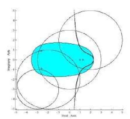
Fig. 4.1. Γ(A)when∆<0, the numerical range and the Gerˇsgorin disks ofA.
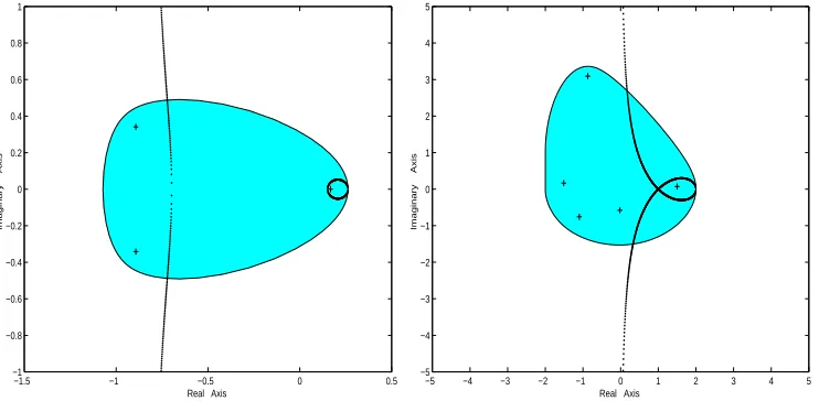
Example 4.4. We have constructed a matrixA∈ M4(C) with v(A) = 17.0173, u(A) = 3.3800 and δ1= 3.5708, δ2=−0.2342.
As ∆ <0, Γ(A) in Figure 4.2 is a simple open curve. A is a non-real matrix and Γ(A) is symmetric with respect to the horizontal line {z ∈ C: Imz = u(A) = 0}. Eigenvalues ofAare marked with +’s.
−10 −8 −6 −4 −2 0 2 4 6
−10 −8 −6 −4 −2 0 2 4 6 8 10
Real Axis
Imaginary Axis
[image:7.612.184.392.437.623.2]Example 4.5. We have constructed matricesAandB with the following data:
A∈ M3(R) with v(A) = 0.1063, u(A) = 0, δ1= 0.2621, δ2=−0.8082;
B∈ M5(C) with v(B) = 1, u(B) = 0, δ1= 2, δ2= 0.
In Figure 4.3, the eigenvalues of each matrix are marked with +’s.
Γ(A) comprises two branches∗, one of which is open and the other a Jordan curve
(∆>0). The closed branch of Γ(A) surrounds a real eigenvalue ofA and the other branch isolates the rest of the spectrum to its left (since all eigenvalues whose real parts are less thanδ2 must lie to the left of Γ(A)).
Γ(B) intersects itself like a folium of Descartes (∆ = 0) whose loop encloses an eigenvalueλwith Reλ > δ1+δ2+
√
∆
2 =s2.All other eigenvalues lie to the left of Γ(B) for the same reason as above.
−1.5 −1 −0.5 0 0.5
−1 −0.8 −0.6 −0.4 −0.2 0 0.2 0.4 0.6 0.8 1
Real Axis
Imaginary Axis
−5 −4 −3 −2 −1 0 1 2 3 4 5
−5 −4 −3 −2 −1 0 1 2 3 4 5
Real Axis
[image:8.612.102.473.299.481.2]Imaginary Axis
Fig. 4.3. Γ(A)has a simple closed branch andΓ(B)is not simple.
Note that whenAis a normal matrix, by the definitions and the fact that left and right eigenvectors ofA coincide, it follows that there existsλ∈σ(A) with Reλ=δ1 and v(A) = Im2λ, u(A) = Imλ.In particular, if Imλ= 0 (e. g. , whenAis Hermitian), thenδ1∈σ(A), namely, an eigenvalue ofAlies on Γ(A).
Our next goal is to identify eigenvalues on Γ(A).For that purpose, denote the circle centered atα∈Cwith radiusr≥0 by
C(α, r) = {s+it:s, t∈R and (s−Reα)2+ (y−Imα)2=r2}.
Theorem 4.6. LetA∈ Mn(C)and λ be an eigenvalue ofAsuch thatλ ∈Γ(A).
Let alsoδ1 > δ2be the two largest eigenvalues of the Hermitian part ofA. Then either
λis a real root of the equation
λ3
−(2δ1+δ2)λ2+ (δ12+ 2δ1δ2+ v(A))λ+ u(A)2(δ1−δ2)−δ1(v(A) +δ1δ2) = 0,
or λ=x+iy /∈C(δ1,u(A)) satisfies the equation
2x3
−(5δ1+δ2)x2+ [2δ1δ2+ 4δ21+ 2y
2+ 2u(A)y]x
−(δ1+δ2)y2−2δ1u(A)y
= (δ1−δ2)u(A)2+δ21(δ1+δ2).
Proof.Letλ =δ1 be an eigenvalue of A with Reλ = δ2, and u, E, H(E), S(E) be as defined in the proof of Theorem 3.1. Equality in (3.1), namely
(Imλ−u(A))2 = (δ
1−Reλ)
v(A)
−u(A)2 Reλ−δ2
+ Reλ−δ1
holds if and only if
Reλ−δ2=
(δ1−Reλ)u∗u (δ1−Reλ)2+ (Imλ−u(A))2
.
(4.4)
In this case, the eigenvalue 0∈σ(H(E)) is simple and corresponds to the eigenvector
u that appears in (3.2). Moreover, the matrix E is singular and 0∈∂F(E) because ReF(E) =F(H(E)). Thus 0 must be a normal eigenvalue ofE (see [5]) and every corresponding eigenvector belongs to Nul(H(E)) ∩ Nul(S(E)) = span{u}. Hence,
u is an eigenvector of S(E) in (3.5) corresponding to the eigenvalue 0 and so
u∗S1u
u∗u = iImλ −
i(Imλ −u(A)) (δ1−Reλ)2+ (Imλ −u(A))2
u∗u.
(4.5)
The same arguments applied to λ ∈σ(A) yields
u∗S1u
u∗u = iImλ −
i(Imλ −u(A)) (δ1−Reλ)2+ (Imλ −u(A))2
u∗u.
(4.6)
We set λ =x+iy and by (4.5), (4.6) we obtain
2y = 2y[(x−δ1) 2+y2
−u(A)2]
[(δ1−x)2+ (y−u(A))2] [(δ1−x)2+ (y+ u(A))2]
u∗u.
(4.7)
From (4.7) we now have two cases: Either
(a) y= Imλ = 0, in which case since λ ∈Γ(A) , we have
u(A)2 = (δ1−λ)
v(A)
−u(A)2
λ−δ2
+λ−δ1
that is, equivalently, λ coincides with the (triple) real root of
λ3
−(2δ1+δ2)λ2+ [δ21+ 2δ1δ2+ v(A)]λ −δ21δ2−δ2u(A)2−δ1(v(A)−u(A)2) = 0;
or
(b) y= 0 and thus (x−δ1)2+y2= u(A)2; in this case (4.7) can be written as
(x−δ1)2+ (y+ u(A))2 (x−δ1)2+y2−u(A)2 =
u∗u
(δ1−x)2+ (y−u(A))2
and so by (4.4) we have
x−δ2 =
(δ1−x) [(x−δ1)2+ (y+ u(A))2] (x−δ1)2+y2−u(A)2 ,
completing the proof.
We can apply the results in the previous section to rotations ofA ∈ Mn(C) in
order to obtain localizations of its spectrum that are complementary to the one ob-tained by Γ(A).For example, we can consider three additional curves, Γ(−A),Γ(iA) and Γ(−iA).The spectrum inclusion region resulting from these curves is illustrated in the next example.
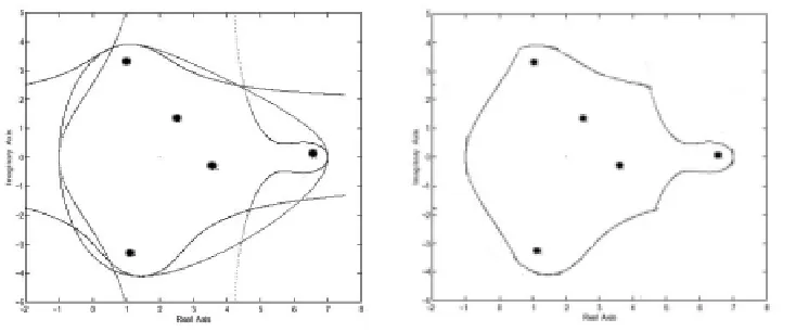
Example 4.7. LetA=
4 0 −1 0 0
0 5 −1 2 3
1 1 2 +i −1 0 0 −2 1 −1 3−i
0 1 0 −3−i 5
. In Figure 4.4, the
[image:10.612.107.474.447.600.2]numerical range and the curves Γ(A), Γ(−A), Γ(iA) and Γ(−iA) are superimposed on the left; on the right the region carved out of the numerical by the four curves is isolated.The eigenvalues ofAare marked with•’s.
Fig. 4.4. Left: the numerical range and Γ(A),Γ(−A),Γ(iA),Γ(−iA)superimposed. Right:
5. Conclusions. We have provided an inequality satisfied by each eigenvalueλ
ofA∈ Mn(C).Upon rotation ofA byπ/2, πand 3π/2, it generalizes the classical
fact generally attributed to Bendixson [1, Theorem II] that
min{µ:µ∈σ(H(A))} ≤ Reλ ≤ max{µ:µ∈σ(H(A))}
and
min{ν:ν∈σ(S(A)/i)} ≤ Imλ ≤ max{ν:ν ∈σ(S(A)/i)}
by replacing the lines represented by these lower and upper bounds with cubic curves. We note that there have been other improvements of Bendixson’s results by replacing the bounding box with circular and hyperbolic regions that depend on all the eigen-values of the Hermitian and skew-Hermitian parts; see Wielandt [8] and references therein.
In our results, the curve Γ(A) depends only on the quantities v(A) and u(A) defined in (2.1), as well as on the two largest eigenvalues ofH(A),δ1 and δ2.As a consequence, the additional computational effort for Γ(A) over Bendixson’s results is reasonably small and with the help of a graphing device, Γ(A) can provide a new efficient localization for the eigenvalues ofA.
We conclude with possible directions for future research:
(1) Consider arbitrary rotationseiθA of A in order to obtain a family of localizing
curves and thus sharper localization results.Specifically, determine the intersection of all the localization regions arising from Theorem 3.1 applied toeiθAasθranges in
[0,2π).This effort appears to be analogous to the characterization of the numerical range as an intersection of half-planes [5, Theorem 1.5.12]. As the computational effort is likely to be substantial for matrices of large order, it may instead be interesting to determine a minimal number of localizing curves so that the intersection of the corresponding regions is contained entirely in the numerical range ofA.
(2) Referring to Observation 4.2 item (4), the notation thereby and the case when Γ(A) is not a simple open curve (∆≥0), investigate the number of eigenvalues ofA
that can lie to the right of the points2 on the lineL={z∈C: Imz= u(A)}.
(3)Recall that whenδ1=δ2, Γ(A) degenerates to a single point.Pursue non-trivial generalizations of Γ(A) when the largest eigenvalue ofH(A) is not simple.Referring to the proof of Theorem 3.1, this may be possible by orthogonally reducing H(A) relative to the entire eigenspace corresponding to its largest eigenvalue.
REFERENCES
[1] I. Bendixson. Sur les racines d’une ´equation fondamentale.Acta Mathematica, 25:359-365, 1902. [2] S. Friedland, Eigenvalues of almost skew-symmetric matrices and tournament matrices. In
Gu-bernatorial and graph-theoretical problems in linear algebra (R. A. Brualdi, S. Friedland,
and V. Klee, Eds), IMA Vol. Math. Appl. 50, Springer-Verlag, New York, 1993, pp. 189–206. [3] S. Friedland and M. Katz. On the maximal spectral radius of even tournament matrices and the spectrum of almost skew-symmetric compact operators.Linear Algebra and its Applications, 208/209:455–469, 1994.
[4] R. Horn and C.R. Johnson.Matrix Analysis, Cambridge University Press, 1990.
[5] R. Horn and C.R. Johnson.Topics in Matrix Analysis, Cambridge University Press, 1991. [6] S. Kirkland, P. Psarrakos, and M. Tsatsomeros. On the location of the spectrum of
hypertour-nament matrices.Linear Algebra and its Applications, 323:37–49, 2001.
[7] J.J. McDonald, P.J. Psarrakos, and M.J. Tsatsomeros. Almost skew-symmetric matrices.Rocky
Mountain Journal of Mathematics, 34:269–288, 2004.