Bethe Ansatz Solutions of the Bose–Hubbard Dimer
⋆Jon LINKS and Katrina E. HIBBERD
Centre for Mathematical Physics, School of Physical Sciences, The University of Queensland, 4072, Australia
E-mail: [email protected], [email protected]
URL: http://www.maths.uq.edu.au/∼jrl/, http://www.maths.uq.edu.au/∼keh/
Received October 26, 2006, in final form December 19, 2006; Published online December 29, 2006 Original article is available athttp://www.emis.de/journals/SIGMA/2006/Paper095/
Abstract. The Bose–Hubbard dimer Hamiltonian is a simple yet effective model for descri-bing tunneling phenomena of Bose–Einstein condensates. One of the significant mathema-tical properties of the model is that it can be exactly solved by Bethe ansatz methods. Here we review the known exact solutions, highlighting the contributions of V.B. Kuznetsov to this field. Two of the exact solutions arise in the context of the Quantum Inverse Scattering Method, while the third solution uses a differential operator realisation of the su(2) Lie algebra.
Key words: Bose–Hubbard dimer; Bethe ansatz
2000 Mathematics Subject Classification: 81R12; 17B80; 81V99
1
Introduction
The experimental realisation of Bose–Einstein condensation using atomic alkali gases has pro-vided the means to study macroscopic tunneling in systems with tunable interation parame-ters [9]. From the theoretical perspective, the Bose–Hubbard dimer model (see equation (1) below), also known as thediscrete self-trapping dimer[4,5,6] or thecanonical Josephson Hamil-tonian[9], has been extremely useful in understanding this tunneling phenomena in the context of a bosonic Josephson junction. Despite its apparent simplicity, the Hamiltonian captures the essence of competing linear and non-linear interactions which lead to non-trivial dynamical be-haviour and ground-state properties (e.g. [7, 12, 14, 15, 16]). In particular the model predicts macroscopic self-trapping and the collapse and revival of Rabi oscillations, features which have been directly observed experimentally in a single bosonic Josephson junction [1,11].
The Bose–Hubard dimer Hamiltonian is given by
H = k
8(N1−N2)
2
−µ2(N1−N2)−E
2(b
†
1b2+b†2b1), (1)
whereb†1,b †
2 denote the single-particle creation operators for two bosonic modes andN1 =b † 1b1, N2 =b†2b2 are the corresponding boson number operators. The couplingkprovides the strength
of the scattering interaction between bosons, µ is the external potential and E is the coupling for the tunneling. The change E → −E corresponds to the unitary transformation b1 → b1, b2 → −b2, while µ → −µ corresponds to b1 ↔ b2. The total boson number N = N1 +N2 is
conserved and consequently the model is integrable as it has only two degrees of freedom and two conserved operators, viz. H andN. Mathematically the Hamiltonian is of interest because, related to its integrability, it admits exact Bethe ansatz solutions. This property opens avenues
to rigorously analyse the model. For example, the Bethe ansatz solution can be used to study the ground-state crossover from a delocalised state to a “Schr¨odinger cat” state in the attractive case [3], as well as facilitating the calculation of form factors [10].
The first Bethe ansatz solution of the Hamiltonian was given by Enol’skii et al. [4,5] using the machinery of the Quantum Inverse Scattering Method. A key ingredient in this approach was the use of a bosonic realisation of the Yang–Baxter algbera, which was developed in the work of Kuznetsov and Tsiganov [8]. For zero external potential an alternative application of the Quantum Inverse Scattering Method, using the Gaudin algebra formulation, was given by Enol’skii, Kuznetsov and Salerno [6]. We remark this method of solution for the model has also been recently discussed in [13,14]. In this approach a connection was made with confluent Heun polynomials. It was also observed in their work [6] that this connection could be established using an su(2) realisation of the Hamiltonian (see also [17]). This property provides a direct route to a third Bethe ansatz solution using elementary properties of second-order ordinary differential eigenvalue equations with polynomial solutions.
2
Exact Bethe ansatz solution I
In this section we review the Quantum Inverse Scattering Method and associated algebraic Bethe ansatz. The notational conventions we adopt follow those of [10], which also contains the full details for the following calculations. Then we will apply this approach to derive the exact Bethe ansatz solution of (1), as was originally described in [4,5].
We begin with thesu(2)-invariantR-matrixR(u)∈End(C2⊗C2), depending on the spectral
parameter u∈C:
R(u) =
1 0 | 0 0
0 b(u) | c(u) 0
− − − −
0 c(u) | b(u) 0
0 0 | 0 1
, (2)
with b(u) =u/(u+η) and c(u) = η/(u+η). Above, η is an arbitrary parameter. It is easy to check that R(u) satisfies the Yang–Baxter equation
R12(u−v)R13(u)R23(v) =R23(v)R13(u)R12(u−v) (3)
on End(C2 ⊗C2
⊗C2). Above R
jk(u) denotes the matrix acting non-trivially on the j-th and
k-th spaces and as the identity on the remaining space. Next we define the Yang–Baxter algebra with monodromy matrixT(u),
T(u) =
A(u) B(u)
C(u) D(u)
(4)
subject to the constraint
R12(u−v)T1(u)T2(v) =T2(v)T1(u)R12(u−v). (5)
Given a representationπ of the monodromy matrix, the transfer matrix is defined
t(u) =π(A(u) +D(u)) (6)
which satisfies [t(u), t(v)] = 0 for any choice of u and v as a result of (3). If there exists a pseudovacuum state |χi which satisfies
π(C(u))|χi 6= 0, π(D(u))|χi=d(u)|χi
the transfer matrix has eigenvalues
Λ(u) =a(u) M
Y
k=1
u−vk+η
u−vk
+d(u) M
Y
k=1
u−vk−η
u−vk
. (7)
Provided the Bethe ansatz equations
a(vk)
d(vk) = M
Y
j6=k
vk−vj−η
vk−vj+η
, k= 1, . . . , M (8)
are satisfied.
We may choose the following realization for the Yang–Baxter algebra, with arbitraryω ∈C,
π(T(u)) =Lb1(u+ω)L
b
2(u−ω) (9)
written in terms of the bosonic realisation of the Lax operator given by Kuznetsov and Tsiga-nov [8]:
Lbi(u) =
u+ηNi bi
b†i η−1
, i= 1,2. (10)
Since L(u) satisfies the relation
R12(u−v)Lbi1(u)Lbi2(v) =Lbi2(v)Lbi1(u)R12(u−v), i= 1,2 (11)
it is easy to check that the relations of the Yang–Baxter algebra (5) are obeyed. Specifically, the realisation of the generators of the Yang–Baxter algebra is
π(A(u)) = (u2 −ω2
)I+ηuN+η2
N1N2−ηω(N1−N2) +b†2b1, π(B(u)) = (u+ω+ηN1)b2+η−1b1,
π(C(u)) =b†1(u−ω+ηN2) +η−1b†2, π(D(u)) =b†1b2+η
−2 I,
It is straightforward to verify the Hamiltonian (1) is related with the transfer matrix (6) through
H =−ρ
t(u)−1 4(t
′(0))2
−ut′(0)−η−2+ω2 −u2
,
where the following identification has been made for the coupling constants:
k
8 =
ρη2
4 ,
µ
2 =−ρηω,
E
2 =ρ.
We can apply the algebraic Bethe ansatz method, using the Fock vacuum |0i as the pseudova-cuum |χi, giving
a(u) =u2−ω2, d(u) =η−2.
For this case the Bethe ansatz equations are
η2
(v2
k−ω
2
) = M
Y
j6=k
vk−vj−η
vk−vj+η
whereM is the eigenvalue of the total number operatorN. The energies of the Hamiltonian are
This last expression is independent of the spectral parameteru, which can be chosen arbitrarily.
3
Exact Bethe ansatz solution II
The second Bethe ansatz solution of (1) described by Enol’skii, Kuznetsov and Salerno [6] applies only when µ= 0, i.e. for the Hamiltonian
H = k
8(N1−N2)
2
− E2(b†1b2+b†2b1). (13)
To obtain this solution, first we introduce new operators through a transformation
b1 =
such that the canonical commutation relations [aj, a†k] =δjkI etc. hold. Under the above trans-formation the Hamiltonian (13) becomes
H = k
The next step is to write (14) in terms of an su(2) realisation. The su(2) algebra has generators {Sz, S±}with relations
[Sz, S±] =±S±, [S+, S−] = 2Sz. (15)
It may be shown that
S+
is ansu(2) realisation preserving the commutation relations (15). It follows that we may write
H = k
To derive the Bethe ansatz solution for (16), one takes
g=
with α∈C, and constructs the monodromy matrix
where β∈Cand
The elements of the monodromy matrix are found to be
π(A(u)) = exp(ηα)
from which we can construct the transfer matrix (6). For the Bethe ansatz solution, the pseudo-vacuum state |χi can be chosen to be the vacuum state |0i, either of the one-particle states
a†1|0i ora
In this manner the form of the Bethe ansatz solution depends on whether the total particle number is even or odd. We find
a(u) = exp(ηα)
are related to the Hamiltonian (16) and the total number operator through
H =τ2−τ1−
Letting λj denote the eigenvalue of τj, it follows from (7) that
The eigenvalues of the Hamiltonian are given by
E =E(κ2−κ1) +
where those of the number operator are
N = 2M+ 2(κ1+κ2)−1.
It is apparent that the Bethe ansatz equations (12) with ω = 0, which are in multiplicative form, take on a different form to those given by (19) which are additive. Moreover, the Bethe ansatz equations (12) are associated with a single reference state whereas (19) are dependent on the choice of reference state. In this latter case there are four forms of the Bethe ansatz equations associated with the choices of κ1,κ2 which can take values 1/4 or 3/4. In the following it will
be shown how a unified system of Bethe ansatz equations can be derived in the additive form. This approach does not use the Quantum Inverse Scattering Method.
4
Exact Bethe ansatz solution III
We again follow the work of Enol’skii, Kuznetsov and Salerno [6] (see also [17]) and start with the Jordan-Schwinger realisation of the su(2) algebra (15):
S+
=b†1b2, S−=b†2b1, Sz =
1
2(N1−N2)
which is (N + 1)-dimensional when the constraint of fixed particle number N = N1 +N2 is
imposed. In terms of this realisation the Hamiltonian (1) may be written as
H = k
The same (N + 1)-dimensional representation of su(2) is given by the mapping to differential operators
acting on the (N + 1)-dimensional space of polynomials with basis {1, u, u2
, . . . , uN}. We can then equivalently represent (20) as the second-order differential operator
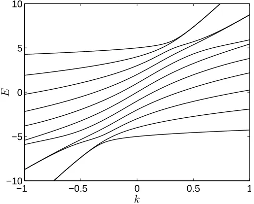
−1 −0.5 0 0.5 1 −10
−5 0 5 10
k
E
Figure 1. Energy levelsE versus couplingkof the Hamiltonian (1) forN= 10,µ= 0, and E= 1.
Solving for the spectrum of the Hamiltonian (1) is then equivalent to solving the eigenvalue equation
HQ(u) =EQ(u), (22)
where H is given by (21) andQ(u) is a polynomial function ofu of orderN.
From this point, it is little effort to obtain a third Bethe ansatz solution for the Hamilto-nian (1) (cf. [3]). First express Q(u) in terms of its roots{vj}:
Q(u) = N
Y
j=1
(u−vj).
Evaluating (22) at u=vl for eachl leads to the set of Bethe ansatz equations
Ev2
l + (k(1−N)−2µ)vl− E
kv2
l
= N
X
j6=l 2
vj−vl
, l= 1, . . . , N. (23)
Writing the asymptotic expansion Q(u) ∼ uN −uN−1 PN
j=1
vj and by considering the terms of
order N in (22), the energy eigenvalues are found to be
E = kN
2
8 −
µN
2 +
E
2 N
X
j=1
vj. (24)
associated with the Bethe ansatz solution (23), (24) there is a mapping of the spectrum of the Hamiltonian into the low energy spectrum of a one-dimensional Schr¨odinger equation. This facilitates a different approach for determining quantum phases of the Hamiltonian where the crossover is identified with a bifurcation of the Schr¨odinger equation potential [3].
Acknowledgements
The work was funded by the Australian Research Council under Discovery Project DP0557949.
[1] Albiez M., Gati R., F¨olling J., Hunsman S., Cristiani M., Oberthaler M., Direct observation of tunneling and non-linear self-trapping in a single bosonic Josephson junction, Phys. Rev. Lett., 2005, V.95, 010402, 4 pages,cond-mat/0411757.
[2] Cirac J.I., Lewenstein M., Molmer K., Zoller P., Quantum superposition states of Bose–Einstein condensates, Phys. Rev. A, 1998, V.57, 1208–1218,quant-ph/9706034.
[3] Dunning C., Hibberd K.E., Links J., On quantum phase crossovers in finite systems,J. Stat. Mech.: Theor. Exp., 2006, P11005, 11 pages,quant-ph/0602098.
[4] Enol’skii V.Z., Salerno M., Kostov N.A., Scott A.C., Alternate quantizations of the discrete self-trapping dimer,Phys. Scripta, 1991, V.43, 229–235.
[5] Enol’skii V.Z., Salerno M., Scott A.C., Eilbeck J.C., There’s more than one way to skin Schr¨odinger’s cat, Phys. D, 1992, V.59, 1–24.
[6] Enol’skii V.Z., Kuznetsov V.B., Salerno M., On the quantum inverse scattering method for the DST dimer, Phys. D, 1993, V.68, 138–152.
[7] Kohler S., Sols F., Oscillatory decay of a two-component Bose–Einstein condensate,Phys. Rev. Lett., 2002, V.89, 060403, 4 pages,cond-mat/0107568.
[8] Kuznetsov V.B., Tsiganov A.V., A special case of Neumann’s system and the Kowalewski–Chaplygin– Goryachev top,J. Phys. A: Math. Gen., 1989, V.22, L73–L79.
[9] Leggett A.J., Bose–Einstein condensation in the alkali gases: some fundamental concepts, Rev. Modern Phys., 2001, V.73, 307–356.
[10] Links J., Zhou H.-Q., McKenzie R.H., Gould M.D., Algebraic Bethe ansatz method for the exact calcula-tion of energy spectra and form factors: applicacalcula-tions to models of Bose–Einstein condensates and metallic nanograins,J. Phys. A: Math. Gen., 2003, V.36, R63–R104,nlin.SI/0305049.
[11] Matthews M.R., Anderson B.P., Haljan P.C., Hall D.S., Holland M.J., Williams J.E., Wieman C.E., Cor-nell E.A., Watching a superfluid untwist itself: recurrence of Rabi oscillations in a Bose–Einstein condensate, Phys. Rev. Lett., 1999, V.83, 3358–3361,cond-mat/9906288.
[12] Milburn G.J., Corney J., Wright E.M., Walls D.F., Quantum dynamics of an atomic Bose–Einstein conden-sate in a double-well potential,Phys. Rev. A, 1997, V.55, 4318–4324.
[13] Ortiz G., Somma R., Dukelsky J., Rombouts S., Exactly-solvable models derived from a generalized Gaudin algebra,Nuclear Phys. B, 2005, V.707, 421–457,cond-mat/0407429.
[14] Pan F., Draayer J.P., Quantum critical behavior of two coupled Bose–Einstein condensates,Phys. Lett. A, 2005, V.339, 403–407,cond-mat/0410423.
[15] Tonel A.P., Links J., Foerster A., Quantum dynamics of a model for two Josephson-coupled Bose–Einstein condensates,J. Phys. A: Math. Gen., 2005, V.38, 1235–1245,quant-ph/0408161.
[16] Tonel A.P., Links J., Foerster A., Behaviour of the energy gap in a model of Josephson-coupled Bose–Einstein condensates,J. Phys. A: Math. Gen., 2005, V.38, 6879–6891,cond-mat/0412214.