COMBINATORICS OF BRANCHINGS IN HIGHER DIMENSIONAL
AUTOMATA
PHILIPPE GAUCHER
ABSTRACT. We explore the combinatorial properties of the branchingareas of
execu-tion paths in higher dimensional automata. Mathematically, this means that we inves-tigate the combinatorics of the negative corner (or branching) homology of a globular
ω-category and the combinatorics of a new homology theory called the reduced branch-ing homology. The latter is the homology of the quotient of the branchbranch-ing complex by the sub-complex generated by its thin elements. Conjecturally it coincides with the non reduced theory for higher dimensional automata, that is ω-categories freely generated by precubical sets. As application, we calculate the branchinghomology of some ω -categories and we give some invariance results for the reduced branching homology. We only treat the branchingside. The mergingside, that is the case of mergingareas of execution paths is similar and can be easily deduced from the branchingside.
1. Introduction
After [22, 14], one knows that it is possible to model higher dimensional automata (HDA) using precubical sets (Definition 2.1). In such a model, a n-cube corresponds to a n-transition, that is the concurrent execution ofn 1-transitions. This theoretical idea would be implemented later. Indeed a CaML program translating programs in Concurrent Pascal into a text file coding a precubical set is presented in [10]. At this step, one does not yet consider cubical sets with or without connections since the degenerate elements have no meaning at all from the point of view of computer-scientific modeling (even if in the beginning of [12], the notion of cubical sets is directly introduced by intellectual reflex).
In [14], the following fundamental observation is made : given a precubical set(Kn)n0 together with its two families of face maps (∂α
i ) for α ∈ {−,+}, then both chain
com-plexes (ZK∗, ∂α), where ZX means the free abelian group generated by X and where ∂α =
i(−1) i+1∂α
i , give rise to two homology theories H∗α for α ∈ {−,+} whose
non-trivial elements model the branching areas of execution paths for α=− and the merging areas of execution paths forα = + in strictly positive dimension. Moreover the group H−
0 (resp. H0+) is the free abelian group generated by the final states (resp. the initial states) of the HDA.
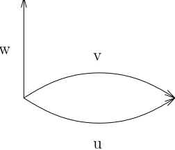
Consider for instance the 1-dimensional HDA of Figure 1. Then u−w gives rise to a non-trivial homology class which corresponds to the branching which is depicted.
Then the first problem is that the category of precubical sets is not appropriate to
Received by the editors 2000 January 29 and, in revised form, 2001 June 27. Transmitted by Ronald Brown. Published on 2001 July 3.
2000 Mathematics Subject Classification: 55U.
Key words and phrases: cubical set, thin element, globular higher dimensional category, branching, higher dimensional automata, concurrency, homology theory.
c
Philippe Gaucher, 2001. Permission to copy for private use granted.
u
v
w x
Figure 1: A 1-dimensional branching area
u
w
Figure 2: A 1-dimensional branching area
identify the HDA of Figure 1 with that of Figure 2because there is no morphism between them preserving the initial state and both final states.
No matter : it suffices indeed to work with the category of precubical sets endowed with the +i cubical composition laws satisfying the axioms of Definition 2.4 and with the
morphisms obviously defined. Now for any n 1, there are n cubical composition laws +1, . . . ,+n representing the concatenation of n-cubes in the n possible directions. Let
X =u+1 v and Y :=w+1x. Then there is a unique morphism f in this new category
of HDA from the HDA of Figure 2to the HDA of Figure 1 such that f : u → X and f :w →Y. However f is not invertible in the category of precubical sets equipped with cubical composition laws because there still does not exist any morphism from the HDA of Figure 1 to the HDA of Figure 2.
To make f invertible (recall that we would like to find a category where both HDA would be isomorphic), it still remains the possibility of formally adding inverses by the process of localization of a category with respect to a collection of morphisms. However a serious problem shows up : the non-trivial cyclesu−w andX−Y of Figure 1 give rise to two distinct homology classes although these two distinct homology classes correspond to the same branching area. Indeed there is no chain in dimension 2(i.e. K2 =∅), so no
way to make the required identification !
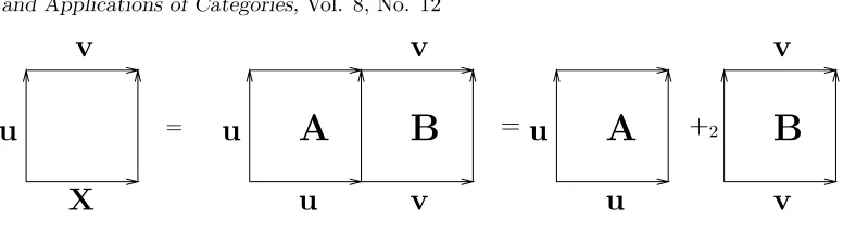
This means that something must be added in dimension 2, but without creating ad-ditional homology classes. Now consider Figure 3. The element A must be understood as a thin 2-cube such that, with our convention of orientation, ∂1−A = u, ∂2−A = u, ∂1+A=ǫ1∂1−v, ∂2+A=∂2−B =ǫ1∂1−v. And the element B must be understood as another thin 2-cube such that∂−
2 B =ǫ1∂1−v,∂2+B =ǫ1∂1+v and ∂1−B =∂1+B =v. In such a
situa-tion, ∂−(A+
2B) = u+1v−u thereforeu+1v andu become equal in the first homology
group H−
1 . By adding this kind of thin 2-cubes to the chain complex (ZK∗, ∂−), one can
cubes which are necessary to treat the branching case. The first kind is well-known in cubical set theory : this is for example B = ǫ1v or ∂1+A = ǫ1∂1−v. The second kind is
for exampleA which will be denoted by Γ−
1u and which corresponds to extra-degeneracy
maps as defined in [6].
To take into account the symmetric problem of merging areas of execution paths, a third family Γ+i of degeneracy maps will be necessary. In this paper, we will only treat
the case of branchings. The case of mergings is similar and easy to deduce from the branching case. The solution presented in this paper to overcome the above problems is then as follows :
• One considers the free globular ω-category F(K) generated by the precubical set K : it is obtained by associating to any n-cube x of K a copy of the free globular ω-category In generated by the faces of the n-cube (paragraph 3.1) ; the faces of
thisn-cube are denoted by (x;k1. . . kn) ; one takes the direct sum of all these cubes
and one takes the quotient by the relations
(∂iαy;k1. . . kn)∼(y;k1. . . ki−1αki. . . kn)
for any y∈Kn+1,α ∈ {−,+} and 1in+ 1.
• Then we take its cubical singular nerve N
(F(K)) (which is equal also to the free cubical ω-category generated by K) ; the required thin elements above described (the three families ǫi, Γ−i and Γ+i ) do appear in it as components of the algebraic
structure of the cubical nerve (Definition 2.4 and Definition 3.3).
• The branching homology ofF(K) (Definition 3.5) is the solution for both following reasons :
1. Let x and y be two n-cubes of the cubical nerve which are in the branching complex. If x+j y exists for some j with 1 j n, then x and x+j y are
equal modulo elements in the chain complex generated by the thin elements (Theorem 9.2) ;
2. The chain complex generated by the thin elements is conjecturally acyclic in this situation, and so it does not create non-trivial homology classes (Conjec-ture 3.6).
We have explained above the situation in dimension 1. The 2-dimensional case is depicted in Figure 8. Additional explanations are available at the end of Section 9.
The branching homology (or negative corner homology) and the merging homology (or positive corner homology) were already introduced in [12]. This invariance with respect to the cubifications of the underlying HDA was already suspected for other reasons. The branching and merging homology theories are the solution to overcome the drawback of Goubault’s constructions.
+2
= =
u
v
u
v
v
v
X
u
v
u
u
A
B
A
B
Figure 3: Identifyingu+1v and u
1. the extra structure ofconnections Γ± on cubical sets, which allow extra degenerate elements in which adjacent faces coincide. This structure was first introduced in [6].
2. the notion of folding operator. This was introduced in the groupoid context in [6], to fold down a cube to an element in a crossed complex, and in the category context in [1] to fold down a cube to an element in a globular category. Properties of this folding operator are further developed in [2]. This we call the ‘usual folding operator’.
3. the notion of thin cube, namely a multiple composition of cubes of the form ǫiy or
Γ±z. A crucial result is that these are exactly the elements which fold down to 1 in the contained globular category.
This paper is organized as follows. Section 2recalls some important notations and con-ventions for the sequel. In Section 3, the branching homology and the reduced branching homology are introduced. In Section 4, the matrix notations for connections and de-generacies are described. Next in Section 5, the branching homology of some particular ω-categories (theω-categories of length at most 1) is completely calculated in terms of the usual simplicial homology. In Section 6, the negative folding operators are introduced. In Section 7, the negative folding operators are decomposed in terms of elementary moves. In Section 8, we prove that each elementary move appearing in the decomposition of the folding operators induces the identity map on the reduced branching complex. Therefore the folding operators induce the identity map as well. In Section 9, the behaviour of the cubical and globular composition laws in the reduced branching complex is completely studied. In the following Section 10, some facts about the differential map in the reduced branching complex are exposed. In the last Section 11, some invariance results for the re-duced branching homology are exposed and the rere-duced branching homology is calculated for some simple globular ω-categories.
2. Preliminaries : cubical set, globular and cubical category
Here is a recall of some basic definitions, in order to make precise some notations and some conventions for the sequel.
2.1. Definition. [6] [16] A cubical set consists of a family of sets(Kn)n0, of a family of
face maps Kn ∂α
i
//Kn−1 forα ∈ {−,+}and of a family of degeneracy maps Kn−1 ǫi //Kn
with 1in which satisfy the following relations
1. ∂α i ∂
β j = ∂
β
j−1∂iα for all i < j n and α, β ∈ {−,+} (called sometimes the cube
axiom)
2. ǫiǫj =ǫj+1ǫi for all ij n
3. ∂α
i ǫj =ǫj−1∂iα for i < j n and α ∈ {−,+}
4. ∂α
i ǫj =ǫj∂iα−1 for i > j n and α∈ {−,+} 5. ∂α
i ǫi =Id
A family (Kn)n0 only equipped with a family of face maps ∂iα satisfying the same axiom
as above is called a precubical set. An element of K0 will be sometimes called a state, or a 0-cube and an element of Kn a n-cube, or a n-dimensional cube.
2.2. Definition. Let (Kn)n0 and (Ln)n0 be two cubical (resp. precubical) sets. Then a morphism f from (Kn)n0 to(Ln)n0 is a familyf = (fn)n0 of set maps fn :Kn→Ln
such that fn∂iα =∂iαfn and fnǫi =ǫifn (resp. fn∂iα =∂iαfn) for any i. The corresponding
category of cubical sets is isomorphic to the category of pre-sheaves Setsop
over a small category . The corresponding category of precubical sets is isomorphic to the category of pre-sheaves Setspreop
2.3. Definition. [5] [26] [24] A (globular) ω-category is a set A endowed with two families of maps (d−
n = sn)n0 and (d+n = tn)n0 from A to A and with a family of partially defined 2-ary operations(∗n)n0 where for anyn 0, ∗n is a map from{(a, b)∈
A×A, tn(a) = sn(b)} to A ((a, b) being carried over a∗nb) which satisfy the following
axioms for all α and β in {−,+} :
1. dβ
mdαnx=
dβ
mx if m < n
dα
nx if mn
2. snx∗nx=x∗ntnx=x
3. if x∗ny is well-defined, then sn(x∗n y) = snx, tn(x∗ny) = tny and for m = n,
dα
m(x∗ny) = dαmx∗ndαmy
4. as soon as the two members of the following equality exist, then (x∗n y) ∗nz =
x∗n(y∗nz)
5. ifm =n and if the two members of the equality make sense, then(x∗ny)∗m(z∗nw) =
(x∗mz)∗n(y∗mw)
6. for any x in A, there exists a natural number n such that snx = tnx = x (the
smallest of these numbers is called the dimension of x and is denoted by dim(x)).
A globular set is a set A endowed with two families of maps (sn)n0 and (tn)n0
satisfying the same axioms as above [27, 21, 3]. We callsn(x) then-source of xand tn(x)
the n-target ofx.
Notation. The category of all ω-categories (with the obvious morphisms) is denoted by ωCat. The corresponding morphisms are called ω-functors. The set of n-dimensional morphisms of C is denoted byCn. The set of morphisms of C of dimension lower or equal
than n is denoted by trnC. The element ofC0 will be sometimes called states. An initial state (resp. final state) of C is a 0-morphism α such that α=s0x(resp. α=t0x) implies
x=α.
2.4. Definition. [6, 1] A cubical ω-category consists of a cubical set
((Kn)n0, ∂iα, ǫi)
together with two additional families of degeneracy maps called connections
Γα
i : Kn //Kn+1
with α ∈ {−,+}, n 1 and 1 in and a family of associative operations +j defined
on {(x, y)∈Kn×Kn, ∂j+x=∂
−
j y} for 1j n such that
1. ∂α i Γ
β j = Γ
β
2. ∂α
The corresponding category with the obvious morphisms is denoted by ∞Cat.
Notation. If S is a set, the free abelian group generated by S is denoted by ZS. By definition, an element of ZS is a formal linear combination of elements of S.
2.5. Definition. [12] Let C be an ω-category. Let Cn be the set of n-dimensional
mor-phisms of C. Two n-morphismsx andy are homotopic if there exists z ∈ZCn+1 such that snz−tnz =x−y. This property is denoted by x∼y.
We have already observed in [12] that the corner homologies do not induce functors fromωCatto the category of abelian groups. A notion of non-contractingω-functors was required.
2.6. Definition. [12] Let f be an ω-functor from C to D. The morphism f is non-contracting if for any 1-dimensional x ∈ C, the morphism f(x) is a 1-dimensional mor-phism of D.
The theoretical developments of this paper and future works in progress entail the following definitions too.
2.7. Definition. Let C be an ω-category. Then C is non-contracting if and only if for any x ∈ C of strictly positive dimension, s1x and t1x are 1-dimensional (they could be a priori 0-dimensional as well).
A justification of this definition among a lot of them is that ifC is anω-category which is not non-contracting, then there exists a morphism u of C such that dim(u) > 1 and such that for instance s1u is 0-dimensional. For example consider the two-element set
{A, α} with the rules s1A =t1A= s0A =t0A= α and s2A =t2A =A. This defines an
ω-category which is not non-contracting. Then A is 2-dimensional though s1A and t1A
are 0-dimensional. And in this situation−2(A) defined in Section 6.5 is not an element of the branching nerve, and therefore for thatC, the morphismCF2−(C) (see Proposition 9.4)
to CR−
2(C) is not defined.
Notation. The category of non-contracting ω-categories with the non-contracting ω-functors is denoted by ωCat1.
If f is a non-contracting ω-functor from C to D, then for any morphism x ∈ C of dimension greater than 1, f(x) is of dimension greater than one as well. This is due to the equality f(s1x) =s1f(x).
All globular ω-categories that will appear in this work will be non-contracting.
3. Reduced branching homology
3.1. The globularω-category In. We need first to describe precisely theω-category
associated to the n-cube. Set n = {1, ..., n} and let cubn be the set of maps from n to
{−,0,+} (or in other terms the set of words of length n in the alphabet {−,0,+}). We say that an element x of cubn is of dimension p if x−1(0) is a set of p elements. The set
cubn is supposed to be graded by the dimension of its elements. The set cub0 is the set of
be the map from (cubn)i to (cubn)dim(y) defined as follows (with x∈ (cubn)i) : for k ∈n,
x(k)= 0 implies ry(x)(k) = x(k) and ifx(k) is thel-th zero of the sequencex(1), ..., x(n),
then ry(x)(k) =y(ℓ). If for any ℓ between 1 and i, y(ℓ)= 0 implies y(ℓ) = (−)ℓ, then we
set by(x) := ry(x). If for any ℓ between 1 and i, y(ℓ) = 0 impliesy(ℓ) = (−)ℓ+1, then we
setey(x) :=ry(x). We have
If x is an element of cubn, let us denote by R(x) the subset of cubn consisting of y ∈cubn such that y can be obtained fromx by replacing some occurrences of 0 in x by
− or +. For example, −00 + +− ∈R(−000 +−) but +000 +−∈/ R(−000 +−). If X is a subset of cubn, then let R(X) = x∈X R(x). Notice that R(X∪Y) =R(X)∪R(Y).
3.2. Theorem. There is one and only one ω-category In such that
1. the underlying set of In is included in the set of subsets of cubn
2. the underlying set of In contains all subsets like R(x) where x runs overcubn
3. all elements of In are compositions of R(x) where x runs over cubn
4. for x p-dimensional with p1, one has
sp−1(R(x)) =R({by(x), dim(y) = p−1})
tp−1(R(x)) =R({ey(x), dim(y) = p−1})
5. if X and Y are two elements of In such that t
p(X) = sp(Y) for some p, then
X∪Y ∈In and X∪Y =X∗ pY.
Moreover, all elements X of In satisfy the equality X =R(X).
The elements of In correspond to the loop-free well-formed sub pasting schemes of the
pasting scheme cubn [15] [9] or to the molecules of anω-complex in the sense of [25]. The condition “X∗nY exists if and only ifX∩Y =tnX =snY” of [25] is not necessary here
because the situation of [25] Figure 2 cannot appear in a composable pasting scheme. The map which sends every ω-category C toN(C)∗ =ωCat(I∗,C) induces a functor from ωCat to the category of cubical sets. If x is an element of ωCat(In,C),ǫ
i(x) is the
ω-functor from In+1 to C defined by ǫ
i(x)(k1...kn+1) = x(k1...ki...kn+1) for all i between
1 and n+ 1 and ∂α
i (x) is the ω-functor from In−1 to C defined by ∂iα(x)(k1...kn−1) =
x(k1...ki−1αki...kn−1) for all i between 1 andn.
The arrow ∂α
i for a given isuch that 1in induces a natural transformation from
ωCat(In,−) to ωCat(In−1,−) and therefore, by Yoneda, corresponds to an ω-functor
δα
i from In−1 to In. This functor is defined on the faces of In−1 by δiα(k1...kn−1) =
R(k1...[α]i...kn−1). The notation [...]i means that the term inside the brackets is at the
i-th place.
3.3. Definition. The cubical set (ωCat(I∗,C), ∂α
i , ǫi)is called the cubical singular nerve
3.4. Remark. For α∈ {−,+}, and x∈ωCat(In,C), let
∂αx:=
n
i=1
(−1)i+1∂iαx
Because of the cube axiom, one has∂α◦∂α = 0.
3.5. Definition. [12] Let C be a non-contracting ω-category. The set of ω-functors
x∈ωCat(In,C) such that for any 1-morphism u with s
0u=−n+1, x(u) is 1-dimensional
(a priori x(u) could be 0-dimensional as well) is denoted by ωCat(In,C)−. Then
∂−(ZωCat(I∗+1,C)−)⊂ZωCat(I∗,C)−
by construction. We set
H−
∗ (C) =H∗(ZωCat(I∗,C)−, ∂−)
and we call this homology theory the branching homology of C. The cycles are called the branchings of C. The map H−
∗ induces a functor from ωCat1 to Ab.
The definition ofωCat(In,C)−is a little bit different from that of [12]. Both definitions coincide if C is the free ω-category generated by a precubical set or a globular set. This new definition ensures that the elementary moves introduced in Section 7 are well-defined on the branching nerve. Otherwise it is easy to find counterexample, even in the case of a non-contracting ω-category.
3.6. Conjecture. (About the thin elements of the branching complex) Let C be a globular ω-category which is either the free globular ω-category generated by a precubical set or the free globular ω-category generated by a globular set. Let xi be elements of
ωCat(In,C)− and let λ
i be natural numbers, where i runs over some set I. Suppose that
for any i, xi(0n)is of dimension strictly lower than n (one calls it a thin element). Then
iλixi is a boundary if and only if it is a cycle.
The thin elements conjecture is not true in general. Here is a counterexample. Con-sider an ω-category C constructed by considering I2 and by dividing by the relations
R(−0) = R(0−) and R(−0) ∗0 R(0+) = R(0−) ∗0 R(+0). Then the ω-functor F ∈
ωCat(I2,C)− induced by the identity functor from I2 to itself is a thin cycle in the
branching homology. One can verify that this cycle would be a boundary if and only if R(0+) was homotopic to R(+0) in C. This observation suggests the following questions.
3.7. Definition. Let C be an ω-category. Then the n-th composition law is said to be left regular up to homotopy if and only if for any morphisms x, y and z such that
x∗ny =x∗nz, then y∼z.
3.8. Question. Does the thin elements conjecture hold for anω-category C such that all composition laws ∗n for any n 0 are left regular up to homotopy ?
3.10. Definition. Let M−
n(C) ⊂ ZωCat(In,C)− be the sub-Z-module generated by the
thin elements (M for “mince” which means “thin” in French). Set
CR−
n(C) = ZωCat(In,C)−/(Mn−(C) +∂−Mn−+1(C)) where M−
n(C) + ∂−M
−
n+1(C) is the sub-Z-module of ZωCat(In,C)− generated by Mn−(C)
and the image of M−
n+1(C) by ∂−. The differential map ∂− induces a differential map
CR−
n+1(C)−→CR−n(C)
This chain complex is called the reduced branching complex ofC. The homology associated to this chain complex is denoted by HR−
∗(C) and is called the reduced branching homology
of C.
3.11. Proposition. Conjecture 3.6 is equivalent to the following statement : if C is the free ω-category generated by a precubical set or by a globular set, then the canonical map from the branching chain complex to the reduced branching chain complex of C is a quasi-isomorphism.
Proof. By the following short exact sequence of chain complexes
0 //M∗−(C) +∂−M−
∗+1(C) //ZωCat(I∗,C)− //CR−∗(C) //0 the assumption H−
n(C) ∼= HR−n(C) for all n is equivalent to the acyclicity of the chain
complex (M−
∗ +∂−M −
∗+1, ∂−) (notice that M0−(C) =M1−(C) = 0).
Now if Conjecture 3.6 holds, then take an element x∈M−
n(C) +∂−M
−
n+1(C) which is
a cycle. Then x = t1+∂−t2 where t1 ∈ Mn−(C) and t2 ∈ Mn−+1(C). Then t1 is a cycle
in ZωCat(In,C)− and a linear combination of thin elements. Therefore t1 is a cycle in ZωCat(In,tr
n−1C)−. By Conjecture 3.6, t1 = ∂−t3 where t3 ∈ ZωCat(In+1,trn−1C)−.
Therefore t1 ∈ ∂−Mn−+1(C). Conversely, suppose that the sub-complex generated by the
thin elements is acyclic. Take a cycle t of ZωCat(In,C)− which is a linear combination of thin elements. Then t is a cycle of M−
n(C) +∂−M
−
n+1(C), therefore there exists t1 ∈
Mn−+1(C) and t2 ∈Mn−+2(C) such that t=∂−(t1+∂−t2) =∂−t1.
3.12. Definition. Let x and y be two elements of ZωCat(In,C)−. Then x and y are
T-equivalent (T for thin) if the corresponding elements in the reduced branching complex are equal, that means if x−y ∈M−
n(C) +∂−Mn−+1(C). This defines an equivalence relation on ZωCat(In,C)− indeed.
4. Matrix notation for higher dimensional composition in the cubical
sin-gular nerve
There exists on the cubical nerve ωCat(I∗,C) of an ω-category C a structure of cubical ω-categories [12] by setting
Γ−
i (x)(k1. . . kn) = x(k1. . .max(ki, ki+1). . . kn)
Γ+
i (x)(k1. . . kn) = x(k1. . .min(ki, ki+1). . . kn)
4.1. Proposition. [12] Let C be a globular ω-category. For any strictly positive natural number n and anyj between1 and n, there exists one and only one natural map +j from
the set of pairs (x, y) of N(C)
n× N(C)n such that ∂j+(x) =∂j−(x) to the set N(C)n
which satisfies the following properties :
∂−
Moreover, these operations induce a structure of cubical ω-category on N(C).
The sum (x+iy) +j(z+it) = (x+j z) +i(y+jt) if there exists will be denoted by
and using this notation, one can write
• If i=j, Γ−i (x+j y) =
The matrix notation can be generalized to any composition like
(a11+i. . .+ia1n) +j. . .+j (am1+i. . .+iamn)
whenever the sources and targets of the aij match up in an obvious sense (this is not
necessarily true). In that case, the above expression is equal by the interchange law to
(a11+j . . .+j am1) +i. . .+i(a1n+j . . .+j amn)
and we can denote the common value by
4.2. Definition. [6][1] A n-shell in the cubical singular nerve is a family of 2(n+ 1)
elements x±
i of ωCat(In,C) such that ∂iαx β j = ∂
β
j−1xαi for 1 i < j n+ 1 and α, β ∈
{−,+}.
4.3. Definition. The n-shell (x±i ) is fillable if
1. the sets {x(i−)i,1 i n+ 1} and {x
(−)i+1
i ,1 i n+ 1} have each one exactly
one non-thin element and if the other ones are thin.
2. if x(i0−)i0 and xi1(−)i1 +1 are these two non-thin elements then there exists u ∈ C such that sn(u) = x(
−)i0
i0 (0n) and tn(u) = x(
−)i1 +1 i1 (0n).
The following proposition is an analogue of [1] Proposition 2.7.3.
4.4. Proposition. [12] Let (x±i ) be a fillable n-shell with u as above. Then there exists
one and only one elementxofωCat(In+1,C)such thatx(0
n+1) =u, and for1in+1, and α∈ {−,+} such that ∂α
i x=xαi.
Proposition 4.4 has a very important consequence concerning the use of the above notations. In dimension 2, an expressionA like (for example)
x y
✲✻1 2
is necessarily equal to
x y
✲2
✻
1
because the labels of the interior are the same (A(00) = (x+2y)(00)) and because the shells
of 1-faces are equal (∂−
1 A=∂1−x, ∂1+A=∂1+x+1∂1+y, ∂2−A=∂2−x,∂2+A=∂1−y+1∂2+y) :
the dark lines represent degenerate elements which are like mirrors reflecting rays of light. This is a fundamental phenomenon to understand some of the calculations of this work. Notice that A=x+2y because ∂1−A=∂1−(x+2y).
All calculations involving these matrix notations are justified because the Dawson-Par´e condition holds in 2-categories due to the existence of connections (see [11] and [7]). The Dawson-Par´e condition stands as follows : suppose that a square α has a decomposition of one edge a as a = a1 +1 a2. Then α has a compatible composition α = α1+i α2, i.e.
such that αj has edge aj for j = 1,2. This condition can be understood as a coherence
condition which ensures that all “compatible” tilings represent the same object.
5. Relation between the simplicial nerve and the branching nerve
5.1. Proposition. [12] Let C be an ω-category and α∈ {−,+}. We setN−
n (C) =ωCat(I
n+1,C)−
and for all n 0 and all 0in,
∂i :Nn−(C) //N
−
n−1(C)
is the arrow ∂−
i+1, and
ǫi :Nn−(C) //N
−
n+1(C) is the arrow Γ−
i+1. We obtain in this way a simplicial set
(N−
∗ (C), ∂i, ǫi)
called the branching simplicial nerve of C. The non normalized complex associated to it gives exactly the branching homology ofC (in degree greater than or equal to 1). The map
N− induces a functor from ωCat
1 to the category Sets∆
op
of simplicial sets.
The globular ω-category ∆n. Now let us recall the construction of the ω-category
called by Street then-th oriental [26]. We use actually the construction appearing in [17]. LetOn be the set of strictly increasing sequences of elements of{0,1, . . . , n}. A sequence
of length p+ 1 will be of dimension p. If σ ={σ0 < . . . < σp} is a p-cell of On, then we
set∂jσ ={σ0 < . . . <σj < . . . < σk}. If σ is an element of On, let R(σ) be the subset of
On consisting of elements τ obtained fromσ by removing some elements of the sequence
σ and letR(Σ) =σ∈ΣR(σ). Notice that R(Σ∪T) =R(Σ)∪R(T).
5.2. Theorem. There is one and only one ω-category ∆n such that
1. the underlying set of ∆n is included in the set of subsets of On
2. the underlying set of ∆n contains all subsets like R(σ) where σ runs over On
3. all elements of ∆n are compositions of R(σ) where σ runs over On
4. for σ p-dimensional with p1, one has
sp−1(R(σ)) = R({∂jσ, j is even})
tp−1(R(σ)) = R({∂jσ, j is odd})
5. if Σ and T are two elements of ∆n such that t
p(Σ) = sp(T) for some p, then
Σ∪T ∈∆n and Σ∪T = Σ∗ pT.
Moreover, all elements Σ of ∆n satisfy the equality Σ =R(Σ).
If C is an ω-category and if x∈ ωCat(∆n,C), then consider the labeling of the faces
• ǫi(x)(σ0 < . . . < σr) =x(σ0 < . . . < σk−1 < σk−1< . . . < σr−1) if σk−1 < i and
σk > i.
• x(σ0 < . . . < σk−1 < i < σk+1−1< . . . < σr−1) ifσk−1 < i,σk =iandσk+1 > i+1.
• x(σ0 < . . . < σk−1 < i < σk+2−1< . . . < σr−1) ifσk−1 < i,σk =iandσk+1 =i+1.
and
∂i(x)(σ0 < . . . < σs) =x(σ0 < . . . < σk−1 < σk+ 1< . . . < σs+ 1)
where σk, . . . , σsi and σk−1 < i.
It turns out that ǫi(x) ∈ ωCat(∆n+1,C) and ∂i(x) ∈ ωCat(∆n−1,C). See [19, 28] for
further information about simplicial sets. One has :
5.3. Definition. [26] The simplicial set (ωCat(∆n,C), ∂
i, ǫi)is called the simplicial
ner-ve N(C) of the globular ω-category C. The corresponding homology is denoted by H∗(C).
5.4. Definition. Let C be a non-contracting ω-category. By definition,C is of length at most 1 if and only if for any morphisms x and y of C such that x∗0y exists, then either
x or y is 0-dimensional.
5.5. Theorem. Let C be an ω-category of length at most 1. D enote by PC the unique ω-category such that its set ofn-morphisms is exactly the set of(n+1)-morphisms ofC for any n0with an obvious definition of the source and target maps and of the composition laws. Then one has the isomorphisms Hn(PC)∼=Hn−+1(C) for n 1.
Proof. We give only a sketch of proof. By definition, H−
n+1(C) = Hn(N−(C)) for n
1. Because of the hypothesis on C, every element x of ωCat(In+1,C)− is determined by the values of the x(k1. . . kn+1) where k1. . . kn+1 runs over the set of words on the
alphabet {0,−}. It turns out that there is a bijective correspondence between On and
the word of length n + 1 on the alphabet {0,−} : if σ0 < . . . < σp is an element of
On, the associated word of length n+ 1 is the word m
0. . . mn such that mσi = 0 and if j /∈ {σ0, . . . , σp}, then mj = −. It is then straightforward to check that the simplicial
structure of N−(C) is exactly the same as the simplicial structure of ωCat(∆∗,PC) in strictly positive dimension 1.
The above proof together with Proposition 5.1 gives a new proof of the fact that if x∈ωCat(∆n,C), the labelings ∂
i(x) and ǫi(x) above defined yieldω-functors from ∆n−1
(resp. ∆n+1) to C.
Notice that the above proof also shows that Hn(PC) ∼= Hn++1(C) where H∗+ is the merging homology functor 2 This means that for an ω-category of length at most 1,
H−
n+1(C) ∼= Hn++1(C) for any n 1. In general, this isomorphism is false as shown by
1The latter point is actually detailed in [13].
2Like the branching nerve, the definition of the merging nerve needs to be slightly change, with respect
to the definition given in [12]. The correct definition is : an ω-functor xfrom In to a non-contracting
ω-categoryCbelongs toωCat(In
,C)+if and only if for any 1-morphismγofIn such that
t0(γ) =R(+n),
BRANCHING MERGING
Figure 4: A case where branching and merging homologies are not equal in dimension 2
Figure 4. The precubical set we are considering in this figure is the complement of the depicted obstacle. Its branching homology is Z⊕Z in dimension two, and its merging homology is Z in the same dimension.
The result Hn(PC) ∼= Hn−+1(C) ∼= Hn++1(C) for C of length at most one and for n 1
also suggests that the program of constructing the analogue in the computer-scientific framework of usual homotopy invariants is complete for this kind of ω-categories. The simplicial set N(PC) together with the graph obtained by considering the 1-category generated by the 1-morphisms of C up to homotopy contain indeed all the information about the topology of the underlying automaton. Intuitively the simplicial set N(PC) is an orthogonal section of the automaton. Theorem 5.5 suggests that non-contracting ω-categories of length at most one play a particular role in this theory. This idea will be deepened in future works.
5.6. Corollary. With the same notation, ifPC is the free globularω-category generated
by a composable pasting scheme in the sense of [15], then H−
n+1(C) vanishes for n 1.
Proof. By [25] Corollary 4.17 or by [17] Theorem 2.2, the simplicial nerve of the ω-category of any composable pasting scheme is contractible.
p1 and any n1, H−
n(2p) = 0.
Proof. It is obvious for n = 1 and for n 2, H−
n(2p) ∼= Hn−1(P2p). But P2p = 2p−1,
therefore it suffices to notice that the (p−1)-simplex is contractible.
5.8. Corollary. For any n 1, let GnA, B be the ω-category generated by two n
-morphisms A and B satisfying sn−1(A) =sn−1(B) and tn−1(A) =tn−1(B). Then
H−
p (GnA, B) = 0
for 0< p < n or p > n and
H−
0 (GnA, B) = Hn−(GnA, B) =Z.
Proof. It suffices to calculate the simplicial homology of a simplicial set homotopic to a (n−1)-sphere.
Let S be a composable pasting scheme (see [15] for the definition and [17] for addi-tional explanations). A reasonable conjecture is that the branching homology of the free ω-category Cat(S) generated by any composable pasting scheme S vanishes in strictly positive dimension. By Conjecture 5.10, it would suffice for a given composable pasting schemeSto calculate the branching homology of thebilocalization Cat(S)[I, F] ofCat(S) with respect to its initial stateI and its final stateF, that is the sub-ω-category of Cat(S) which consists of the p-morphismsxwithp1 such that s0x∈I and t0x∈F and of the
0-morphism I and F. The question of the calculation of
H−
p+1(Cat(S)[I, F])∼=Hp(PCat(S)[I, F])
for p1 seems to be related to the existence of what Kapranov and Voevodsky call the derived pasting scheme of a composable pasting scheme [17]. It is in general not true thatPCat(S)[I, F] (denoted by ΩCat(S) in their article) is the free ω-category generated by a composable pasting scheme. But we may wonder whether there is a “free cover” of ΩCat(S) by some Cat(T) for some composable pasting scheme T. This T would be the derived pasting scheme of S.
As for the n-cube In, its derived pasting scheme is the composable pasting scheme
generated by the permutohedron [20, 4, 18]. Therefore one has
5.9. Proposition. Denote byIn[−
n,+n]the bilocalization ofInwith respect to its initial
state −n and its final state +n, Then for all p1, Hp−(In[−n,+n]) = 0.
Proof. It is clear that H−
1 (In[−n,+n]) = 0. For p 2, Hp−(In[−n,+n]) ∼= Hp−1(ΩIn)
by Theorem 5.5. But ΩIn is the free ω-category generated by the permutohedron, and
with Corollary 5.6, one gets H−
By filtrating the 1-morphisms ofInby their length, it is possible to construct a spectral
sequence abutting to the branching homology of In. More precisely a 1-morphism x is
of length ℓ(x) if x = R(x1)∗0 . . . ∗0 R(xℓ(x)) where x1, . . . , xℓ(x) ∈ (cubn)1. Now let
FpωCat(I∗, In)− be the subset of x∈ ωCat(I∗, In)− such that for any k1. . . k∗ ∈ (cub∗)1
such that +∈ {k1, . . . , k∗},ℓ(x(k1. . . k∗))p. Then one gets a filtration on the branching
complex of In such that
F−1ZωCat(I∗, In)− ⊂F0ZωCat(I∗, In)− ⊂. . .⊂FnZωCat(I∗, In)−
with
F−1ZωCat(I∗, In)− = 0
F0ZωCat(I∗, In)− = ZωCat(I∗, In(−n,+n))−
FnZωCat(I∗, In)− = ZωCat(I∗, In)−.
One has E1
pq =Hp+q(FpZωCat(I∗, In)−/Fp−1ZωCat(I∗, In)−) =⇒Hp−+q(In). By
Proposi-tion 5.9, E0q= 0 if q= 0 and E00=Z.
The above spectral sequence probably plays a role in the following conjecture :
5.10. Conjecture. Let C be a finite ω-category (that is such that the underlying set is finite). Let I be the set of initial states of C and let F be the set of final states of C (then
H−
0 (C) = H0−(C[I, F]) = ZF). If for any n > 0, Hn−(C[I, F]) = 0, then for any n > 0,
H−
n(C) = 0.
By [17], Ω∆n = In−1, therefore the vanishing of the branching homology of In−1 in
strictly positive dimension and Conjecture 5.10 would enable to establish thatH−
p (∆n) =
0 for p >0 and for any n.
6. About folding operators
The aim of this section is to introduce an analogue in our framework of the usual folding operators in cubicalω-categories. First we show how to recover the usual folding operators in our context.
The notations 0 or −0 (resp. 1 or −1) correspond to the canonical map from C0
toωCat(I0,C) (resp. from tr
1C toωCat(I1,C)). Now let us recall the construction of the
operators −
n of [12].
6.1. Proposition. [12] Let C be an ω-category and let n 1. There exists one and only one natural map −n from trnC to ωCat(In,C) such that the following axioms hold :
1. one has ev0nn=IdtrnC where ev0n(x) =x(0n) is the label of the interior of x.
2. if n3 and 1in−2, then ∂i±−n = Γ
−
n−2∂
±
i
−
n−1sn−1.
3. ifn2andn−1in, then ∂−
i −n =
−
n−1d (−)i
n−1 and∂i+−n =ǫn−1∂n+−1−n−1sn−1.
Moreover for 1i n, we have ∂±
i −nsn =∂i±−ntn and if x is of dimension greater or
6.2. The usual folding operators. One defines a natural map n from Cn to
ωCat(In,C) by induction onn 2as follows (compare with Proposition 6.1).
6.3. Proposition. For any natural number n greater or equal than 2, there exists a unique natural map n from Cn to ωCat(In,C) such that
1. the equality n(x)(0n) = x holds.
2. one has ∂α
1n=n−1d(
−)α
n−1 for α=±.
3. for 1< in, one has ∂α
i n=ǫ1∂iα−1n−1sn−1.
Moreover for 1in, we have ∂±
i nsnu=∂i±ntnu for any (n+ 1)-morphism u.
Proof. The induction equations define a fillable (n−1)-shell (see Proposition 4.4).
6.4. Proposition. For alln0, the evaluation mapev0n :x→x(0n)fromωCat(I
n,C)
to C induces a bijection from γN(C)
n to trnC where γ is the functor defined in [1]. Proof. Obvious for n= 0 and n= 1. Recall that γ is defined by
(γG)n ={x∈Gn, ∂jαx∈ǫ j−1
1 Gn−j for 1j n, α = 0,1}
Let us suppose that n2and let us proceed by induction on n. Sinceev0nn(u) =u by the previous proposition, then the evaluation mapev fromγN(C)
n to trnC is surjective.
Now let us prove that x ∈ γN(C)
n and y ∈ γN(C)n and x(0n) = y(0n) = u imply
x=y. Since x and y are in γN(C)
n, then one sees immediately that the four elements
∂±
1 x and∂1±y are in γN(C)n−1. Since all other ∂iαxand ∂iαy are thin, then ∂
−
1 x(0n−1) =
∂−
1 y(0n−1) = sn−1u and ∂1+x(0n−1) = ∂1+y(0n−1) = tn−1u. By induction hypothesis,
∂1−x = ∂1−y = n−1(sn−1u) and ∂1+x = ∂+1y = n−1(tn−1u). By hypothesis, one can
set ∂α jx = ǫ
j−1
1 xαj and ∂jαy = ǫ j−1
1 yjα for 2 j n. And one gets xαj = (∂1α)j−1∂jαx =
(∂α
1)jx = (∂1α)jy=yjα. Therefore ∂jαx=∂jαy for all α ∈ {−,+} and all j ∈[1, . . . , n]. By
Proposition 4.4, one gets x=y.
The above proof shows also that the map which associates to any cubexof the cubical singular nerve of C the cube dim(x)(x(0dim(x))) is exactly the usual folding operator as
exposed in [1].
Unfortunately, these important operators are not internal to the branching complex, due to the fact that ann-cubexof the cubical singular nerve is in the branching complex if and only for any 1-morphism γ of In starting from the initial state −
n of the n-cube,
x(γ) is 1-dimensional (see Definition 3.5). But for example (n(x(0n)))(−. . .− 0) is
0-dimensional.
6.5. The negative folding operators. The idea of the negative folding operator Φ−
n is to “concentrate” an-cube x of the cubical singular nerve of anω-categoryC to the
faces δ−
6.6. Definition. Set Φ−
n(x) = −n(x(0n)). This operator is called the n-dimensional
negative folding operator.
It is clear that x∈ ωCat(In,C)− implies Φ−
n(x)∈ωCat(In,C)−. Therefore Φ−n yields
a map from ωCat(In,C)− to itself. Since∂−
n−1−n =−n−1d (−)n−1
n−1 and∂n−−n =−n−1d (−)n
n−1, the effect of−n(x(0n)) is indeed
to concentrate the faces of the n-cube x on the faces δ−n−1(0n−1) and δ−n(0n−1). All the
(n−1)-cubes ∂α
i−n(x) for (i, α) ∈ {/ (n−1,−),(n,−)} are thin. Of course there is not
only one way of concentrating the faces of x on δ−
n−1(0n−1) and δn−(0n−1). But in some
way, they are all equivalent in the branching complex (Corollary 8.4). We could decide also to concentrate the n-cubes for n 2on the faces δ−
1(0n−1) and δ2−(0n−1), or more
generally to concentrate the n-cubes on the faces δ−
p(n)(0n−1) and δ−q(n)(0n−1) where p(n)
and q(n) would be integers of opposite parity for all n 2. Let us end this section by explaining precisely the structure of all these choices.
In an ω-category, recall that d−
n =sn, d+n = tn and by convention, let d−ω = d+ω =Id.
All the usual axioms of globular ω-categories remain true with this convention and the partial ordern < ω for any natural numbern.
If x is an element of an ω-category C, we denote by x the ω-category generated by x. The underlying set of x is{snx, tnx, n∈N}. We denote by 2n any ω-category freely
generated by one n-dimensional element.
Let R(k1. . . kn) ∈ In a face. Denote by evk1...kn the natural transformation from ωCat(In,−) to tr
ω which maps f to f(R(k1. . . kn)).
6.7. Definition. Let n ∈ N. Recall that trn is the forgetful functor from ω-categories
to sets which associates to any ω-category its set of morphisms of dimension lower or equal than n and let in be the inclusion functor from trn−1 to trn. We call cubification of
dimension n, or n-cubification a natural transformation from trn to ωCat(In,−). If
moreover, ev0n=Id, we say that the cubification is thick.
We see immediately that −n, n (and +n of [12]) are examples of thick
n-cubifica-tions. By Yoneda the set ofn-cubifications is in bijection with the set of ω-functors from In to 2
n. So for a given n, there is a finite number of n-cubifications.
6.8. Proposition. Let f be a natural transformation from trm to trn with m, n∈N∪
{ω}. Then there exists p m and α ∈ {−,+} such that f = dα
p. And necessarily,
pInf(m, n).
Proof. Denote by
<A>= 2n g
−−−→ <B>= 2m
the ω-functor which corresponds to f by Yoneda. Then g(A) = dα
p(B) for some p and
some α. And necessarily, p min(m, n) (where the notation min means the smallest element).
6.9. Corollary. Let be a n-cubification with n1 a natural number. Then for any
Proof. We have
∂±
i snx(l1. . . ln−1) =evl1...[±]i...ln−1sn(x)
But evl1...[±]i...ln−1 is a natural transformation from trn to trn−1. By Proposition 6.8, we
get
∂±
i snx(l1. . . ln−1) =evl1...[±]i...ln−1tn(x) = ∂
±
i tnx(l1. . . ln−1)
We arrive at a theorem which explains the structure of all cubifications :
6.10. Theorem. Let be a thick n-cubification and let f be an ω-functor from In+1 to
In such that f(R(0
n+1)) =R(0n). D enote by f∗ the corresponding natural transformation
from ωCat(In,−) to ωCat(In+1,−). Then there exists one and only one thick (n+ 1) -cubification denoted by f∗. such that for 1in+ 1,
(f∗.)i
n+1 =f∗
where in+1 is the canonical natural transformation from trn to trn+1.
Proof. One has
∂α
i (f∗.) = ∂iα(f∗.)d(−)
i
n
= ∂α
i (f∗.)in+1d(−)
i
n
= ∂α
i f∗d(−)
i
n
Therefore if x∈ Cn+1 for some ω-categoryC, then ∂iα(f∗.)x =∂iαf∗d
(−)i
n x for 1i
n+ 1 and we obtain a fillable n-shell in the sense of Proposition 4.4.
6.11. Corollary. Letu be anω-functor fromIn to2
nwhich maps R(0n) to the unique
n-morphism of 2n (we will say that u is thick because the corresponding cubification is
also thick). Let f be an ω-functor from In+1 to In which maps R(0
n+1) to R(0n). Then
there exists one and only one thick ω-functor v from In+1 to 2
n+1 such that the following diagram commutes :
In+1 v //
f
2n+1
In u //2 n
the arrow from2n+1 to 2n being the uniqueω-functor which sends the (n+ 1)-cell of 2n+1 to the n-cell of 2n.
If is a n-cubification and fi thick ω-functors from In+i+1 to In+i for 0 i
p then we can denote without ambiguity by fp.fp−1. . . . .f0. the (n +p)-cubification
fp.(fp−1.(. . . .f0.)). Let us denote by0the unique 0-cubification. We have the following
6.12. Proposition. Let x∈ C be a p-dimensional morphism with p1 and let np. Then
−nx= Γ−
n−1. . .Γ−p−px
(by convention, the above formula is tautological for n =p)
Proof. We are going to show the formula by induction on n. The casen =pis trivial. If in−1, then∂i±
Proof. It is an immediate consequence of Proposition 6.12and of the uniqueness of Theorem 6.10.
The converse of Theorem 6.10 is true. That is :
6.14. Proposition. Let v be a thick ω-functor from In+1 to 2
n+1. Then there exists
an ω-functor f such that for any thick ω-functor u from In to 2
n, the following diagram
commutes :
Here is an example of cubification : if the following picture depicts the 3-cube,
we can represent a 3-cubificationby indexing each face k1k2k3 by the corresponding
value ofevk1k2k3i3 which is equal to sd or td for some d between 0 and 2. So let us take
Now let us come back to our choice. It is not completely arbitrary anyway because the operator−
n satisfies the following important property : ifuis an-morphism withn 2,
then −n(u) is a simplicial homotopy within the branching nerve between −n−1(sn−1u)
and −n−1(tn−1u). Moreover, the family of cubifications (−n)n0 is the only family of
cubifications which satisfies this property because it is equivalent to defining an-shell for alln. However most of the results of the sequel can be probably adapted to any family of n-cubification, provided that they yield internal operations on the branching nerve (see Conjecture 7.7 and 7.8).
6.15. Characterization of the negative folding operators. Now here is a useful property of the folding operators :
6.16. Theorem. Let C be an ω-category. Let x be an element of N
n(C). Then the
following two conditions are equivalent :
1. the equality x= Φ−
by induction for n 3. By hypothesis, as soon as + ∈ {k1, . . . , kn}, then x(k1. . . kn) is
6.17. Corollary. The folding operator Φ−
n is idempotent.
The end of this section is devoted to the description of Φ−
2 and Φ−3. Since∂1−−2 =1s1
because the 2-source of R(000) in I3 looks like
R(00−) R(0 + 0) R(−00)
and
because the 2-target of R(000) in I3 looks like
R(+00)
R(0−0) R(00+)
So by convention, an element x of ωCat(I3,C) will be represented as follows
x= A B
3Beware of the fact thatA, . . . F are elements of the cubical singular nerve whereas Gis an element
7. Elementary moves in the cubical singular nerve
In this section, the folding operators Φ−
n are decomposed in elementary moves. First of
all, here is a definition.
7.1. Definition. The elementary moves in the n-cube are one of the following operators (with 1in−1 and x∈ωCat(In,C)) :
Proposition 7.2expresses the elementary moves using the notation of the previous paragraph (only the operators used in the sequel are calculated).
hψ−
2 x=
A B
C
G =⇒
D E F
θ1−x=
A B
C G
=⇒
D
E F
Proof. One has vψ+
i x= Γ+i ∂
−
i x+i x. Therefore
∂−
1
v
ψ1+x=ǫ1∂1−∂1−x
∂1+ vψ+
1(x) = ∂1+x
∂−
2 vψ1+x=ǫ1∂1−∂1−x+1 ∂2−x
∂+
2 vψ1+x=∂1−x+1 ∂2+x
∂3± vψ1+x=∂3±Γ+1∂1−x+1∂3±x
So one has
v
ψ+1x=
A B
C G
=⇒
D
E F
And
∂−
1 vψ2+x= Γ+1∂1−∂2−x+1∂1−x
∂2− vψ2+x=ǫ2∂2−∂2−x
∂3− vψ2+x=ǫ2∂2−x+2∂3−x
∂1+ vψ2+x= Γ+1∂1+∂2−x+1∂1+x
∂2+ vψ2+x=∂2+x ∂3+ vψ+
2x=∂2−x+2 ∂3+x
Consequently one has
v
ψ2+x=
A B
C G
=⇒
D
E F
One has vψ−
i x=x+iΓ−i ∂i+x. Therefore
∂−
1 vψ2−x=∂1−x+1 ∂1−Γ−2∂2+x
∂1+ vψ2−x=∂1+x+1 ∂1+Γ−2∂2+x
∂2− vψ2−x=∂2−x ∂2+ vψ2−x=ǫ2∂2+∂2+x
∂−
3
v
ψ−
2x=∂3−x+2 ∂2+x
∂3+ vψ−
So
vψ−
2 x=
A B
C G
=⇒ D
E F
And
∂−
1
v
ψ−
1x=∂1−x
∂1+ vψ−
1x=ǫ1∂1+∂1+x
∂−
2 vψ1−x=∂2−x+1 ∂1+x
∂+
2 vψ1−x=∂2+x+1 ǫ1∂1+∂1+x
∂3− vψ1−x=∂3−x+1 Γ−1∂2−∂1+x
∂3+ vψ1−x=∂3+x+1 Γ−1∂2+∂1+x
therefore
v
ψ1−x= A B C
G
=⇒ D
E F
One has hψ−
1x=x+2Γ−1∂2+x. Then
∂1− hψ1−x=∂1−x+1∂2+x
∂1+ hψ1−x=∂1+x ∂−
2
h
ψ−
1 x=∂2−x
∂2+ hψ−
1 x=ǫ1∂1+∂2+x
∂−
3 hψ1−x=∂3−x+2Γ−1∂2−∂2+x
∂+
3 hψ1−x=∂3+x+2Γ−1∂2+∂2+x
So
hψ−
1x=
A
B C
G
=⇒ D
E F
One has hψ−
2x=x+3Γ−2∂3+x. Therefore
∂−
1 hψ2−x=∂1−x+2Γ−1∂1−∂3+x
∂1+ hψ2−x=∂1+x+2Γ−1∂1+∂3+x
∂2− hψ2−x=∂2−x+2∂3+x
∂2+ hψ2−x=∂2+x+2ǫ2∂2+∂3+x
∂−
3
h
ψ−
2 x=∂3−x
∂3+ hψ−
so
The following proposition describes some of the commutation relations satisfied by the previous operators, the differential maps and the connection maps.
∂i−+1θ
−
i =∂
−
i+1 (15)
∂i++1θi−=ǫi+1∂i++1∂i−+iǫi+1∂i++1∂i++1 (16)
∂i−+2θ
−
i =
∂−
i+2 ∂i++1
∂i−
✲i+1 ✻
i
(17)
∂i++2θi−= v
ψi+∂i++2 (18)
θ−
i Γ
−
i = Γ
−
i+1 (19)
θ−
i Γ
−
i+1 = Γ−i+1 (20)
Proof. Equalities (1), (2), (3) and (4) are obvious. Equalities from (5) to (12) are immediate consequences of the definitions. With Proposition 7.2, one sees that
∂1−θ1−= Γ−1∂1−∂1− ∂1+θ1−= vψ1−∂1+ ∂−
2 θ1−=∂2−
∂2+θ−
1 =ǫ2∂2+∂1−+1ǫ2∂2+∂2+
∂−
3 θ1−=
∂3− ∂2+ ∂1−
✲2
✻
1
∂3+θ1−= vψ1+∂3+
For a given x, the above equalities are equalities in the free cubical ω-category gener-ated by x. Therefore, they depend only on the relative position of the indices 1, 2and 3 with respect to one another. Therefore, we can replace each index 1 byi, each index 2by i+ 1 and each index 3 by i+ 2to obtain the required formulae.
In the same way, it suffices to prove the last two formulae in lower dimension and for i= 1. One has
θ−
1Γ−1x = θ−1 x
x(00)
=⇒ x
= x x(00)
=⇒ x
= Γ−2x
and
θ1−Γ−2x = θ−1 x x(00)
=
generated byx, and therefore
= (vΨ−1 hΨ−1). . .(vΨ−n−1
Why does the proof of Theorem 7.4 work. The principle of the proof of Theo-rem 7.4 is the following observation (see in [2]) : let f1, . . . , fn be n operators such that
(the product notation means the composition)
1. for anyi, one has fifi =fi (the operators fi are idempotent)
2. |i−j|2implies fifj =fjfi
3. fifi+1fi =fi+1fifi+1 for any i
Then the operatorF =f1(f2f1). . .(fnfn−1. . . f1) satisfiesfiF =F for anyi. This means
thatF enables to apply allfi a maximal number of times. It turns out that the operators vψ±
i and hψ
±
i satisfy the above relations : 7.5. Proposition. The operators vψα
i and hψ β
j are idempotent. Moreover for any
i1 and any j 1, with |i−j|2, the following equalities hold :
Proof. Equalities 21 and 22 are obvious.
For the sequel, one can supposeα =−. In the cubical singular nerve of an ω-category, two elements A and B of the same dimension n are equal if and only if A(0n) = B(0n)
equivalent to proving it for the case i= 1 and to replacing each index 1 by i, each index 2in byi+ 1 and each index 3 byi+ 2 . And in the casei= 1, the equality is a calculation in the free cubical ω-category generated by x. So we can suppose that x is of dimension as low as possible. In our case, this equality makes sense if xis 3-dimensional. Therefore it suffices to verify Equality 23 in dimension 3 for i= 1. And one has
= hψ−
2 A B
C G
=⇒ D
E F
= A B
C
G
=⇒ D
E F
= vψ−
1
A B
C
G =⇒
D E F
= vψ1− hψ2− A B C
G =⇒
D E F
In the same way, to prove Equality 24, it suffices to prove it for i = 1 and in the 3-dimensional case. And one has
v
ψ−1 vψ−2 vψ−1 A B C
G =⇒
D E F
= vψ−
1 vψ2− A B
C G
=⇒ D
E F
= vψ−
1 A B
C G
=⇒ D
E F
=
A B C
G =⇒
D
E F
and
v
ψ2− vψ−1 vψ−2 A B C
G =⇒
D E F
= vψ−
2
v
ψ−
1
A B
C G
=⇒ D
= vψ2− A B
In the same way, one can verify that
hψ−
We are going to prove that
Φ−
n = Θ n−2
n−2Θnn−−32. . .Θn1−2(vΨ1− hΨ−1). . .(vΨ−n−1 hΨ−n−1)
by verifying that the second member satisfies the characterization of Theorem 6.16. Let x∈ωCat(In,C)−. Theorem 7.4 implies that for 1 in, the dimension of
is zero (or equivalently that it belongs to the image of ǫn−1
1 ). With Proposition 7.3, one
for any y∈ωCat(In,C)−. One has
mations of set-valued functors from ωCat(In,−)− to itself.
7.7. Conjecture. Let f be an ω-functor from In to itself such that f(0
n) = 0n and
such that the corresponding natural transformation from ωCat(In,−) to itself induces a
natural transformation Φ− from ωCat(In,−)− to itself. Then Φ− is a composition of
7.8. Conjecture. Let Φ be a natural transformation from ωCat(In,−) to itself such
that the corresponding functor (Φ)∗ from In to itself satisfies (Φ)∗(0
n) = 0n. Then Φ is a
composition of vψ±
i and hψ
±
i for 1in−1.
By Yoneda, the operators vψ±
i and hψ
7.9. Conjecture. Letf be an ω-functor from In to itself such that f(0
We claim that the above construction is sufficient to prove that xand hψ−
1 (x) are
T-equivalent for anyx∈ωCat(In,C)− and for anyn 2. The labeled 3-cubey
1 is actually
a certain thin 3-dimensional element of the cubical ω-categoryN(C) and it corresponds
to the filling of a thin 2-shell. So
y1 =f1(ǫ1x, ǫ2x, ǫ3x,Γ1−x,Γ−2x,Γ+1x,Γ+2x)
where f1 is a function which only uses the operators +1, +2, and +3. In this particular
case, f1 could be of course calculated. But it will not be always possible in the sequel to
make such a calculation : this is the reason why no explicit formula is used here. And one has ∂−
2 f1(x) = x, ∂3−f1(x) = hψ−1(x) and all other 2-faces ∂iαf1(x) are (necessarily)
thin 2-faces. The equalities ∂2−f1(x) = x and ∂3−f1(x) = hψ1−(x) do not depend on
the dimension of x. Therefore for any x ∈ ωCat(In,C)− and for any n 2, one gets ∂−y
1 = hψ−1(x)−x+t where t is a linear combination of thin elements.
Now we want to explain that the above construction is also sufficient to prove that x and hψ−
i (x) are T-equivalent for anyi1 and anyx∈ωCat(In,C)− and for anyn 2.
The equalities∂−
2 f1(x) =xand ∂3−f1(x) = hψ1−(x) do not depend on the absolute values
1, 23. But only on the relative values 1 = 3−2 , 2 = 3−1 and 3 = 3−0. So let us introduce a labeled (n+ 1)-cube yi = fi(x) by replacing in f1 any index 1 in by i, any
index 2by i+ 1 and any index 3 by i+ 2. Then one gets a thin (n+ 1)-cube yi =fi(x)
such that ∂i−+1fi(x) =x and ∂i−+2fi(x) = hψi−(x).
If the reader does not like this proof and prefers explicit calculations, it suffices to notice that y1 = hψ1−Γ−2x by Proposition 7.2. Set yi = hψi−Γ−i+1x. Then
∂−(yi) =
j<i
(−1)j+1 hψi−−1Γ
−
i ∂
−
j x+ (−1) i+1(Γ−
i ∂
−
i x+iǫi+1∂i++1x) +
(−1)i+2(x− hψ−
i x) +
j>i+2
(−1)j+1 hψ−
i Γ
−
i+1∂j−−1x
and one completes the proof by an easy induction on the dimension of x(0n).
8.2. Proposition. For any i 1 and any n 2, if x ∈ ωCat(In,C)−, then vψ−
i (x)
and x are T-equivalent.
Proof. It suffices to make the proof for i= 1 andn = 2. And to consider the following thin 3-cube
x
x(00)
=⇒ x
Notice that the above 3-cube is exactly vψ−
2Γ
−
1x by Proposition 7.2.
8.3. Proposition. For any i1 and any n 3, if x ∈ωCat(In,C)−, then θ−
i (x) and
Proof. It suffices to make the proof for i= 1 and n= 3. Set
x= A B
C G =⇒
D E F
One has already seen that
θ1−x=
A B
C G
=⇒
D
E F
It suffices to construct a thin 4-cube y such that ∂3−y = x and ∂2−y = θ−1x. If the 4-cube is conventionally represented by Figure 5, the thin labeled 4-cube of Figure 6 with 00+0→(∂+2∂−
1 x+1∂2+∂2+x)(0) meets the requirement. The latter labeled 4-cube can be
defined as the unique thin 4-cube ω(x) which fills the 3-shell defined by
∂−
1ω(x) = Γ−2∂1−x
∂−
2ω(x) =θ1−(x)
∂−
3ω(x) =x
∂−
4ω(x) =
Γ−
2∂3−x ǫ2∂2+x
Γ1−Γ+1∂1−∂2+x+2ǫ1Γ−1∂
−
1∂2+x Γ
−
1∂
−
1 x
✲3 ✻
1
∂1+ω(x) = vψ−2Γ−1∂1+x ∂2+ω(x) = Γ−
2∂2+x
∂3+ω(x) =ǫ3(Γ−1∂2+∂1−x+1ǫ2∂2+∂+2x)
∂4+ω(x) = vψ+
2Γ−2∂3+x
8.4. Corollary. For any n 2, for any x ∈ ωCat(In,C)−, x and Φ−
n(x) are
T-equivalent and Φ−
n is the identity map on the reduced branching complex.
We have proved that for any x ∈ ωCat(In,C)−, there exists t
1 ∈ Mn and t2 ∈ Mn+1
such that Φ−
n(x)−x= t1+∂−t2. The proofs of this section use only calculations in the
free cubical ω-category generated by x. This means that t1 and t2 can be formulated in
terms of expressions in the same cubical ω-category. And so this means that t1 and t2
are linear combinations of expressions which use onlyxas variable and the operators ∂±
i ,
Γ±
i , ǫi and +i. With Theorem 7.6 which allows to consider Φ−n like an operator defined
in any cubical ω-category, one sees that Corollary 8.4 does make sense in an appropriate cubical setting. Moreover the termst1 andt2being elements of the free cubicalω-category
+ + 00
D