Understanding Differences in
Household Financial Wealth between
the United States and Great Britain
James Banks
Richard Blundell
James P. Smith
a b s t r a c t
In this paper, we describe the household wealth distribution in the United States and United Kingdom over the past two decades, and compare both wealth inequality and the form in which wealth is held. Unconditionally, there are large differences in financial wealth between the two countries at the top fifth of the wealth distribution. Even after controlling for age and income differences between the two countries, we show that the me-dian U.S. household accumulates more financial wealth than their United Kingdom counterpart does. We explore a number of alternative reasons for these differences and reject some explanations as implausible. Some of the observed differences are due to what we refer to as ‘‘initial condi-tions,’’ in particular previously high rates of corporate equity ownership in the U.S. and housing ownership among young British households. This only provides a partial explanation, however. Among other explanations are differences in the annuitization of retirement incomes and in the amount of wealth held in the form of housing equity. In the first case, forced and voluntary annuitization in the United Kingdom mean older households face considerably less longevity risk. In the second, higher James Banks and Richard Blundell are professors of economics at the Institute for Fiscal Studies and University College, London. James P. Smith is a Senior Economist at RAND. The first two authors gratefully acknowledge the support of the Leverhulme Trust for funding the Institute for Fiscal Studies (IFS) research programme entitled ‘‘The changing distribution of consumption, economic resources and the welfare of households,’’ of which this study forms a part. Cofunding has been provided by the Economic and Social Research Council (ESRC) Centre for the Microeconomic Analysis of Fiscal Pol-icy at IFS. Many thanks are also due to NOP Financial for providing us with the Financial Reporting System (FRS) data used in this study. Neither the ESRC, the Leverhulme Trust, nor NOP Financial bear any responsibility for the analysis or interpretation of the data reported here. Smith’s research was supported by grants from the National Institute on Aging in the United States. Expert program-ming assistance of David Rumpel is gratefully acknowledged. Any remaining errors are attributable to the authors alone. Addresses for correspondence: j.banks@ifs.org.uk;r.blundell@ucl.ac.uk;smith@ rand.org;
[Submitted March 2001; accepted July 2002]
ISSN 022-166X2003 by the Board of Regents of the University of Wisconsin System
242 The Journal of Human Resources
house price volatility in the United Kingdom can create an incentive, as shown Banks, Blundell, and Smith (2002), away from stock market equity earlier in the life cycle.
I. Introduction
Economists have conducted considerable theoretical and empirical research during the last decade on the motives underlying household decisions garding optimal paths of consumption, savings, and wealth accumulation. This re-search has been decidedly international in the sense that scholars from many coun-tries have investigated many diverse country settings. But very little of this existing research has explicitly used cross-national patterns and differences in household wealth to enrich our understanding about what are the primary determinants of these household choices. This is unfortunate in that there are institutional and policy pa-rameters impacting wealth accumulation that vary mainly across and not within country settings. As such, comparative research may be able to exploit a greater source of variation than research on one country alone. In our particular case, a number of central questions could be examined with such an analysis: Are the rea-sons for savings unique to specific nations or do some savings motives transcend national boundaries? Are the citizens of some countries ‘‘savers’’ while the citizens of others ‘‘spenders’’? Are the forms in which wealth is accumulated similar across countries? Do institutions and national policies matter for aggregate national sav-ings? Of course, such comparative research needs to control adequately for covariates that may differ across countries, or across population groups within countries. Hence, it will typically require microdata at the individual or household level. In the case of variables relating to dynamic choices, such as saving and wealth accumulation, such comparisons are further enhanced if the data are of a panel design.
In this paper, we document in detail differences between U.S. and British financial wealth distributions and also attempt to shed light on potential explanations for these differences. Although we will show that comparable microdata exists for the two countries, the data for the United Kingdom are more limited in the sense that only one cross-section is currently available for researchers so that a longitudinal dimension is lacking in the British data.1Consequently, certain hypotheses that we are able to investigate in the United States can only be investigated in Britain on a pseudo-panel basis (using a time-series of cross-sections drawn from a different data source) and others cannot be examined at all. Given what one can learn from the types of analysis presented in this paper, comparable data with a longitudinal dimension would offer even further enhanced opportunities for detailed comparative work, par-ticularly when dealing with issues such as saving, where cohort, age, and time effects all combine to produce trends and patterns in the population.
A number of comparative studies have looked at difference in incomes, wages, and employment patterns between the United States and Britain using a variety of cross-sectional and panel datasets. Few have looked at either savings or wealth, however, and these have typically not used microdata at all. Comparisons that do
Banks, Blundell, and Smith 243
exist suggest that although some differences exist in median financial wealth between the United States and Europe, by far the most striking differences are in the upper middle of the wealth distribution.2These differences are observed between the United States and Britain despite the fact that both appear to have similarly developed fi-nancial systems. In addition, some econometric evidence suggests that consumption-smoothing models for working-age households work equally well across the two countries.3But this evidence exists only for models estimated at the cohort, or cohort and education, specific means, and hence may say little about the behavior at various quantiles of the wealth distribution.
In this paper, we examine microdata from the Panel Study of Income Dynamics and the British Household Panel Study in detail, grouping potential reasons for marked differences in financial wealth dispersion across countries into broad catego-ries. There are a set of issues concerning the importance of measurement and institu-tional factors in generating differences in the wealth distribution across countries. As with any comparative exercise, these have to be dealt with on a specific basis, but differences in the policy regime (both past and future) can play an important role. For example, since saving and wealth levels reflect anticipated future consump-tion needs, to the extent these are diminished by differential provision of social security or health care at different points in the wealth distribution, there may be less incentive to accumulate wealth for precautionary or retirement reasons.
A second set of possible explanations is that the dynamic economic environment facing households differs substantially across countries. Consumption smoothing, through saving or wealth accumulation, is a response to an inherently dynamic pro-cess; past experiences as well as expectations about the future affect the cross-sectional distribution of wealth. There are several motives for saving and wealth accumulation, including intertemporal consumption smoothing (to provide income in retirement, funds for the education of children), precautionary saving (to cover potential periods of poor health or unemployment), and the desire to leave bequests to children. The housing market creates further savings incentives both through the level of down payment required on mortgages and the degree of house price volatil-ity.4 The importance of these motives will depend on both household preferences and the economic environment in which they make their decisions. The dynamics of income processes may be important, and panel data are essential in picking up differences across countries. The degree of deterministic growth in individual income processes, coupled with the persistence and the (conditional) variance of shocks to household income, may be central in driving wealth accumulation and hence wealth dispersion. Equally salient may be household composition, as it will determine spending needs across the life cycle.
Another explanation, and one on which we focus in some detail, may relate to differences in ‘‘initial conditions’’ across the two wealth distributions. Differences in levels and trends in rates of return across countries would lead to increasing differ-ences in inequality across time. But this divergence will be amplified if there are
2. See, for example, the country papers presented at National Academy of Sciences international panel on aging, London, October 1999, summarized in National Academy of Science(2001).
3. See Attanasio and Weber (1993, 1995) for empirical evidence in each country.
244 The Journal of Human Resources
initial differences across countries in the prevalence of ownership of assets where differentials in rate of return are largest. Such an explanation is natural when thinking about the high returns to risky assets (predominantly equity) in the 1980s and 1990s. Only recently (post 1988) has the United Kingdom had substantial levels of direct share ownership in comparison to the United States, and even then, the direct hold-ings of equity of many stockholders are small.
In this paper, we focus almost entirely on financial wealth. In order to understand broader differences in wealth levels one needs to examine housing equity and pen-sion savings. We have chosen to focus on financial wealth because this is the central source of liquidity for families across their working life and a direct measure of the resources available to households. Housing equity and pensions will clearly be important in a complete measure of wealth accumulation, and this needs to be borne in mind when interpreting financial wealth differences across countries. Evidence of the relationship between financial wealth differences and housing equity differ-ences is provided in Banks, Blundell, and Smith (2002a). Using the same data and a similar comparative methodology, they show that although home ownership rates are, on average, similar across the two countries, there are important differences between the United States and Britain. In particular, British households enter the housing market at a younger age, and typically accumulate net housing equity more rapidly than their U.S. counterparts through early stages of the life cycle despite weaker tax incentives for home ownership (or more specifically mortgage interest payments) in Britain. These differences in housing wealth profiles are shown to be consistent with differences in the volatility of the housing market across the two countries.
II. Data Sources
To make wealth comparisons between the United Kingdom and the United States, we rely on two microdata sources that represent among the best at-tempts in each country to improve measurement of household wealth for the entire age distribution. For the United States, we use the Panel Study of Income Dynamics (PSID), which has gathered almost 30 years of extensive economic and demographic data on a nationally representative sample of approximately 5,000 (original) families and 35,000 individuals who live in those families. Unlike many other prominent American wealth surveys, the PSID is representative of the complete age distribution. Wealth modules were included in the 1984, 1989, and 1994 waves of the PSID and all four waves are examined here.
For the United Kingdom, we use the British Household Panel Survey (BHPS). The BHPS has been running annually since 1991 and, like the PSID, is also represen-tative of the complete age distribution. The Wave 1 sample consisted of some 5,500 households, and continuing representativeness of the survey is maintained by follow-ing panel members wherever they move in the United Kfollow-ingdom and also by includfollow-ing in the panel the new members of households formed by original panel members.
house-Banks, Blundell, and Smith 245
hold level, we construct a household wealth definition from the Wave 5 information to use in what follows. Hence, we draw a subsample of households from the BHPS for whom the head and the spouse (where relevant) remain present, and who success-fully complete the wealth module in 1995. This results in a total of 4,688 households, who are each observed in the panel for between one and eight waves.
One question involves whether the two wealth modules are comparable. Appendix Table A1 contains a side-by-side account of the elements that comprise household wealth. Besides housing equity, PSID nonhousing assets are divided into seven cate-gories: other real estate (which includes any second home); vehicles; farm or business ownership; stocks, mutual funds, investment trusts, and stocks held in Individual Retirement Accounts (IRAs); checking, savings accounts, CDs, treasury bills, sav-ings bonds, and liquid assets in IRAs; bonds, trusts, life insurance, and other assets; and other debts. PSID wealth modules include transaction questions about purchases and sales so that active and passive (capital gains) savings can be distinguished.5
While the BHPS detail on assets is similar to those available in PSID, there are some salient differences.6Neither survey oversamples high income or wealth house-holds which—given the extreme skew in the wealth distribution—implies that both surveys understate the concentration of wealth among the extremely wealthy. While this lack of a high wealth oversample is typically a limitation in describing wealth distributions, it has the advantage here of greater comparability between the datasets. Another limitation common to both countries is that neither provides any measure of private pension or government pension wealth.
There are differences between the surveys in how financial asset wealth was col-lected. Both surveys collect information in four broad classes but the classes are slightly different in each country. The PSID uses checking accounts, stocks, other saving (predominantly bonds) and debts, whereas the BHPS uses bank accounts, savings accounts, investments, and debts. For each of these BHPS classes, there are a series of dummy variables recording whether each individual has funds in a particular component of each category. In addition, for investments a variable records which of the various subcomponents is the largest. The following procedure is used to make the wealth categories comparable when disaggregate data are necessary. First, bank accounts and savings accounts are aggregated in the BHPS data. Second, we subdi-vide investments as follows: For individuals who report no ownership of either Na-tional Savings Bonds, NaNa-tional Savings Certificates or Premium Bonds we code their entire investment wealth as shares (27 percent who report owning investment wealth). For those who report no ownership of shares, mutual funds, Personal Equity Plans, or ‘‘Other’’ investments, we code their entire investment wealth as bonds (44 percent of those with investment wealth). For those reporting both ‘‘types’’ of
5. The PSID was the first study to use unfolding brackets to reduce the missing data problem that has plagued surveys with wealth modules. The value of unfolding brackets is not simply in reducing item nonresponse, but in obtaining more accurate measures of asset values. Juster and Smith (1997) conclude that this device increases estimates of total nonhousing net worth by 20 percent for the HRS sample. Unfolding brackets are also used for BHPS financial wealth measures, but other components of net worth were collected using a banded question (secondary housing wealth) or simple point values (housing and vehicles).
246 The Journal of Human Resources
investment wealth (28 percent of those with any investments), we allocate wealth entirely to either shares or bonds, according to the asset type of the largest asset.
One important issue where comparability needs to be established is over retirement savings. Neither survey collects detailed information on state pension wealth or on private (employer) pensions. In the PSID wealth data, however, IRA wealth is in-cluded whereas in the BHPS wealth in the form of Personal Pensions (the nearest comparator to IRAs) is not. Strictly, from a measurement point of view, this is not as problematic as it might seem. In the United Kingdom, Personal Pensions (as well as employer pensions) are a privatealternativeto social security—individuals who choose to contribute to such schemes forfeit their rights to accrue benefits within the state earnings related pension scheme (SERPS). Such private pension contribu-tors have a fraction of their social security contributions rebated and redirected into their personal pension accounts. What is more, for the first few years following the introduction of personal pensions in 1988, most individuals did not make additional contributions over and above these social security contribution rebates (see Inland Revenue 2000 or Disney, Emmerson, and Wakefield 2001, for example). This was still somewhat true for contributors in 1995, and it is certainly not unreasonable to assume that accumulated stocks at this point largely reflect past social security re-bates. Hence, one would not want to include them when constructing a definition of financial wealth to match to the United States where such wealth is unmeasured.7 Most important, an issue of comparability arises over the unit of assessment to which the wealth module applies. It is not possible to get a single estimate of house-hold wealth in any subcategory of financial wealth from the BHPS. This is because every individual was asked to complete the wealth questionnaire, and having reported a total amount for, say, investments, was then asked ‘‘Are any of your investments jointly held with someone else?’’ This framework creates obvious problems in gener-ating a measure of household wealth. We address this issue with a bounding ap-proach. For each of the financial wealth categories in the BHPS two measures are reported. First, we compute an upper bound, assuming that any jointly held asset class is held solely by the individual (the limit of the case where the individual owns ‘‘most’’ of the asset). Second, we compute a lower bound assuming that an individual only owns 1/Nth of the asset class in which joint ownership is reported, whereN is the number of adults in the household. To compute the upper bound of net financial wealth, we add the upper bounds for the asset components and subtract the lower bound of the debt component, and vice versa for the lower bound. In this paper, both lower and upper bound estimates are presented. Fortunately, our conclusions are not sensitive to how this problem is resolved.
Data do not exist to evaluate relevant explanations for differences in several di-mensions of the wealth distribution in the United States and the United Kingdom. Hence, where necessary we also supplement our analysis by the use of other cross-sectional or short panel surveys, such as the Financial Research Survey and the Family Expenditure Survey in the United Kingdom and the Survey of Consumer Expenditures (SCF) in the United States.
Banks, Blundell, and Smith 247
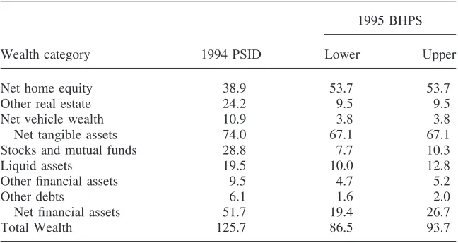
Table 1
Mean Household Wealth and Components in the United States and United Kingdom, 1995 US$, thousands
1995 BHPS
Wealth category 1994 PSID Lower Upper
Net home equity 38.9 53.7 53.7
Other real estate 24.2 9.5 9.5
Net vehicle wealth 10.9 3.8 3.8
Net tangible assets 74.0 67.1 67.1
Stocks and mutual funds 28.8 7.7 10.3
Liquid assets 19.5 10.0 12.8
Other financial assets 9.5 4.7 5.2
Other debts 6.1 1.6 2.0
Net financial assets 51.7 19.4 26.7
Total Wealth 125.7 86.5 93.7
III. Comparing Wealth Distribution in the United
States and Britain
In this section, we describe the main characteristics of household financial wealth distributions in the United Kingdom and United States, highlighting both the similarities and differences. Because the BHPS wealth module was only fielded during the fifth wave (1995), we initially confine our cross-section compari-sons to the 1994 wave of the PSID. Simple summary statistics such as means and medians can be quite misleading when the subject is wealth. Hence, attributes of the full wealth distribution in each country will also be highlighted. To deal with currency differences, the U.K. data (collected in September 1995) are converted into U.S. dollars using the then exchange rate of 1.5525 and all financial statistics for both countries are presented in 1995 U.S. dollars.8
Table 1 lists mean values of wealth and its components for both countries. The striking difference between United Kingdom and United States lies in financial wealth where mean values in America are more than twice those in Britain. These differences exist in all components of financial wealth, but they are particularly large in stock market equity. On average, in the mid-1990s American households owned almost $20,000 more in corporate equity.
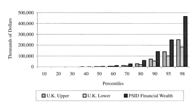
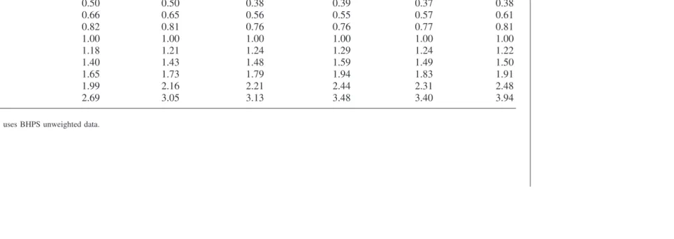
Given the extreme skew in wealth distributions, means are treacherous summary statistics to use for household wealth. Full financial wealth distributions are described in Figure 1. Before highlighting across-country differences, it is worth noting some key similarities. Most important, financial wealth distributions in both countries are
248 The Journal of Human Resources
Figure 1
Net Financial Wealth at Income Percentiles
very unequally distributed. Most American and British households have very few financial assets, but a few have a great deal more. Median financial wealth in both countries is only a few thousand dollars. Again, the real story involves extreme dispersion with relatively few households possessing most of the financial assets. In the United States and the United Kingdom, the top 5 percent have about more than 50 times the level of financial assets of the median household. Of course, reliance on the PSID and BHPS understates the extent of total wealth inequality in each country because both surveys exclude the super-rich in their sampling frames.
Turning to the differences between the countries, Figure 1 illustrates that these differ-ences do not emerge for the typical or median household since median financial assets are only slightly greater among American households. Rather the critical differences lie in the upper tails of the respective financial wealth distribution. No matter which assumption about joint or separate ownership of assets is made in the BHPS, the top fifth of American households have considerably more financial wealth than the top fifth of British households do. Moreover, the between-country discrepancy in financial wealth expands rapidly as we move up the respective financial wealth distributions. The 98thpercentile numbers are more than a quarter of a million dollars apart.
The data in Table 1 and Figure 1 point to the principal research question addressed in this paper. Why do the wealthiest fifth of American households hold so much more financial wealth than the wealthiest fifth of British households? In the next section, we outline some possible factors that could provide answers to this question.
IV. Explaining Wealth Differences
Banks, Blundell, and Smith 249
wealth distributions in their respective populations. We conclude that measurement issues are quite unlikely to explain the principal differences between the countries.
A second class of potential explanations relates to the possibility that measured differences in unconditional distributions reflect differences in wealth covariates across households rather than differences in the wealth accumulation of truly ‘‘simi-lar’’ households. The obvious factors here are differences in the age-structure of the population, as well as differences in income levels or dispersion within age groups. To the extent that these factors cannot fully explain observed differences in wealth distributions (which they do not), we then consider other potential explanations.
Throughout our analysis we keep in mind the possible influence of what we refer to as ‘‘initial conditions.’’ That is, we consider the possibility that current differences in wealth distributions largely reflect past differences that have either persisted, or even been amplified, over the past 10 or 20 years; as opposed to current differences in wealth accumulating behavior across countries. For example, one question is simply whether these financial wealth distributions reflect much higher amounts of financial inheritances received by higher-income American households. Our answer to that will be a definitive no. A second initial condition argument is that differences in wealth distributions in the past have been amplified by the inequality-increasing effect of high returns on risky assets. The argument here is that American households held a greater share of financial wealth in equity on the stock market in the early 1980s and the subsequent ‘‘unexpected’’ growth in equity prices created wider dif-ferences in financial wealth in the 1990s. This initial portfolio allocation toward stock market equity in the United States in the early 1980s coupled with the subsequent macroshock to equity prices does indeed play a significant role but, we will argue, it fails to fully explain intercountry differences in financial wealth.
This then points us toward more behavioral differences between the two countries in their decisions about how much to consume and how much wealth to accumulate over the life cycle, which may also help explain why differences in initial stocks of financial assets arise in the first place. A primary example concerns the much greater reluctance of British households in the past to invest in equity markets. In addition, we also explore reasons why typical as well as atypical households in the two coun-tries may desire to accumulate different amounts of financial wealth over their life cycle. These reasons include differences in the financial consequences of the various risks faced by households (health, or longevity risk, for example) that may produce different levels of ‘‘precautionary savings,’’ differences in bequest motives, ences in markets as a result of transactions costs, taxes or annuity markets, differ-ences in the housing market, and the possibly different roles played by government and occupation pensions in providing income security during old age.
V. Data Comparability
250 The Journal of Human Resources
concentrated.9Although neither sample provides a reliable estimate of mean population wealth, estimates of mean wealth are not our goal. The principal comparability question involves whether the two surveys accurately depict all but the top 1 or 2 percent of wealth holders. The PSID gives a quite good measure of the bottom 99.5 percent of the wealth distribution.10While there is less evidence about the BHPS, a few points are worth noting. Most important, as shown below, BHPS financial wealth data closely mimic financial wealth data in other recently collected wealth surveys in the United Kingdom. Thus, there appears to be nothing unique in the sampling frame used, its panel nature, or questions asked in the BHPS, which distorts financial wealth distribu-tions within the range of our interest. But without a large-scale official survey on house-hold wealth (such as the Survey of Consumer Finances), it is difficult to address the issue of wealth-related differential sample response in the BHPS more directly. Cer-tainly, the use of sample weights ought to correct for known dimensions of nonresponse, but the degree to which these weights (computed on the basis of region, dwelling type, and socioeconomic group) capture nonresponse or attrition by wealth is not known.
The addition of a wealth instrument in the fifth wave of BHPS does not appear to have resulted in any additional attrition in the panel. To get a broader idea of this we look at attrition by education group, which we assume is positively associated with wealth. The results are mixed. Encouragingly, overall levels of attrition are certainly no higher after the wealth module than before, and are fairly low overall, with recontact rates of more than 90 percent after Waves 1 and 2. On the other hand, the attrition occurring at or after the wealth module does appear to be differentially associated with higher education households. Those with education at or above A-levels are significantly more likely to attrit after the wealth module than those with education below A-levels. We evaluated this question with a difference in difference approach. A probit for attrition (that is, individual not present in the following year) that includes year and education dummies and a treatment variable taking the value 1 for an educated indi-vidual observed at or after the wealth module in 1995. This yields a marginal effect on the treatment variable of 0.041 with standard error 0.006.11To the extent that attrition is controlled for by the cross-sectional sample weights, differential attrition will not affect our analysis, which is based on the 1995 cross-section, rather than the longitudinal changes taking place after 1995. We are most encouraged by the comparability of the BHPS financial wealth distribution with those obtained from other cross-sectional surveys collected at the same time in Great Britain.
VI. Controlling for Age and Income Differences
A. Age and the Life-Cycle
Since wealth accumulation is a life-cycle process, unconditional comparisons may be misleading if age structures in the United States and United Kingdom differ. To
9. The PSID contains a low-income oversample that the BHPS does not, but the use of frequency weights in each survey ought to control for this.
10. See, Juster, Smith, and Stafford (1999).
Banks, Blundell, and Smith 251
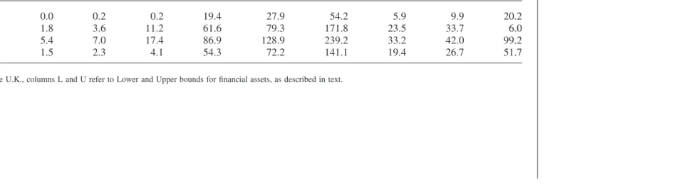
see if age differences underpin wealth differences we condition on three broad age groups of the head of household—(less than 40, 40 to 59, and 60 or over).12Table 2 presents estimates of mean, median, and 90thpercentiles of net financial assets by these broad age groups. If anything, the age split exacerbates differences between the two countries. In all age groups, the mean and 90th percentiles in the United States are much higher than in the United Kingdom. This ranking is also true for median financial wealth in all but the youngest age group. Among those older than age 40, even the median household has more financial wealth in the United States. Equally interesting is to compare wealth inequality within age groups. The ratio of the 90thto the 50thpercentile within age groups tells a different story than the 90/ 50 ratios across all households. In the youngest age group, the United States exhibits much more dispersion than the United Kingdom, but the reverse is true for those age groups above 40, primarily because financial wealth held at the median in the United States has increased rapidly to an extent not observed in the United Kingdom. These extreme patterns are in contrast to the unconditional ratio, which suggests that the United States is more unequal than the United Kingdom (with wealth concen-trated at the top end relative to the median) but not by nearly so much.
Of course, given that at this stage we are treating both the 1994 PSID and 1995 BHPS as cross-sections, differences in wealth across age groups cannot be inter-preted as life cycle patterns. Indeed the possibility of cohort effects distorting such a picture is not unrelated to the initial-conditions argument that we will explore below.
B. Income Levels and Income Inequality
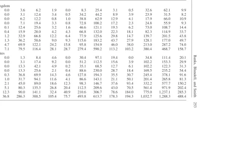
Income is an important determinant of both savings and wealth accumulation. The data in Table 3 show that, within our three age groups, financial. wealth in both countries increases with household disposable income in a highly nonlinear way. Below the median income household in each age group, median financial wealth increases are small as income rises, but then this association becomes quantitatively larger as we move to the highest income households. In both countries for those ages 40–59, median wealth in the highest income decile is more than three times larger than median wealth in the eighth income decile.
Can absolute income differences between the countries as well as higher income inequality in the United States account for much larger financial wealth holdings by American households? Table 4 highlights differences in income dispersion by listing for each country within income decile median incomes relative to median household income. Columns 4 and 6 give income inequality measures for the survey years corresponding to the wealth data in our comparison. While the United Kingdom and United States differ very little in overall levels of income inequality, U.S. income dispersion is higher, especially in the upper two deciles of the income distributions. While U.S. median household income exceeds that in the United Kingdom by 28 percent, the percent gap rises to 44 percent at the 90thpercentile and 75 percent at the 99thpercentile. For issues concerning household savings and wealth, the only
252
The
Journal
of
Human
Resources
Table 2
Net Financial Assets by Broad Age Band of Head of Household, 1995 US$, thousands
Median 90th Percentile Mean
U.K. U.S. U.K. U.S. U.K. U.S.
Age Band L U L U L U
⬍40 0.0 0.2 0.2 19.4 27.9 54.2 5.9 9.9 20.2
40–59 1.8 3.6 11.2 61.6 79.3 171.8 23.5 33.7 6.0
60⫹ 5.4 7.0 17.4 86.9 128.9 239.2 33.2 42.0 99.2
All 1.5 2.3 4.1 54.3 72.2 141.1 19.4 26.7 51.7
Banks,
Blundell,
and
Smith
253
Table 3
Percentiles of Net Financial Wealth and Mean Net Financial Wealth, by Decile of Household Disposable Income Within Broad Age Groups, 1995 US$, thousands
Age⬍40 Age 40–59 Age 60⫹
Income
Decile 50 90 95 Mean 50 90 95 Mean 50 90 95 Mean
United Kingdom
1 0.0 3.6 6.2 1.9 0.0 8.3 25.4 3.1 0.5 32.6 62.1 9.9
2 0.0 3.1 12.4 3.4 0.5 34.2 44.2 8.9 3.9 23.9 31.5 8.2
3 0.0 6.2 12.2 0.8 1.0 38.8 62.9 12.9 4.1 17.9 66.0 10.9
4 0.0 7.1 19.4 3.3 0.8 72.8 100.2 17.2 2.3 24.8 55.9 9.3
5 0.1 12.4 25.6 3.2 1.6 46.6 121.1 19.3 6.2 73.0 108.7 14.4
6 0.4 15.9 28.0 4.2 4.3 66.8 132.0 22.3 18.1 82.3 114.9 33.7
7 1.2 32.9 66.8 12.2 6.4 77.9 125.6 29.8 14.7 139.7 201.5 43.8
8 1.3 36.2 58.6 9.0 9.3 115.6 183.2 43.7 27.9 128.1 177.0 49.7
9 4.7 69.9 122.1 24.2 15.8 95.8 154.9 46.0 38.0 213.0 287.2 74.0
10 7.1 79.5 116.4 28.1 28.7 279.4 590.2 113.2 103.2 380.4 468.7 158.7
United States
1 0.0 1.3 8.4 4.6 0.0 30.4 97.1 19.4 0.0 34.8 111.4 20.1
2 0.0 3.1 17.4 9.2 0.0 51.2 112.5 15.6 3.9 102.2 153.3 29.9
3 0.0 13.3 42.1 4.9 0.2 35.1 68.5 12.7 6.1 102.2 122.3 31.3
4 0.0 13.3 25.6 2.1 0.4 88.6 230.0 28.7 18.4 169.5 235.2 54.4
5 0.3 36.8 69.9 14.3 4.6 127.8 194.3 35.5 30.7 245.4 378.1 91.6
6 1.0 31.7 94.1 11.6 4.1 86.6 143.1 21.1 50.1 201.4 265.8 81.3
7 2.1 45.0 89.0 18.6 12.3 98.3 146.7 37.6 93.4 332.2 577.7 150.2
8 5.1 80.3 135.3 26.8 20.4 112.5 209.6 43.0 70.5 561.4 971.9 202.4
9 12.3 90.0 141.1 32.4 40.9 210.6 306.7 78.6 184.0 775.0 1,237.1 285.3
254
The
Journal
of
Human
Resources
Table 4
Income inequality in the United States and United Kingdom, Ratio of median income within income deciles to median income within 5th decile
(1) (2) (3) (4) (5) (6)
1984 1995 1995 1995 1984 1994
Income Decile FES FES BHPS* BHPS PSID PSID
1 0.37 0.35 0.24 0.26 0.20 0.16
2 0.50 0.50 0.38 0.39 0.37 0.38
3 0.66 0.65 0.56 0.55 0.57 0.61
4 0.82 0.81 0.76 0.76 0.77 0.81
5 1.00 1.00 1.00 1.00 1.00 1.00
6 1.18 1.21 1.24 1.29 1.24 1.22
7 1.40 1.43 1.48 1.59 1.49 1.50
8 1.65 1.73 1.79 1.94 1.83 1.91
9 1.99 2.16 2.21 2.44 2.31 2.48
10 2.69 3.05 3.13 3.48 3.40 3.94
Banks, Blundell, and Smith 255
Figure 2
Median Financial Wealth at Income Percentiles
aspect of dispersion that really matters is at the upper end, since that is where most of the wealth is concentrated in both countries.
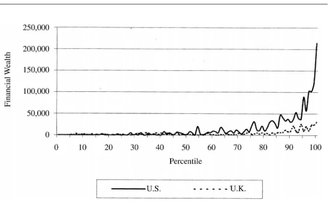
Figure 2 illustrates one way of controlling for both intercountry differences in income levels and dispersion. This figure plots median financial wealth by percentiles of household income in both countries where the solid line represents the United States, and the dashed the United Kingdom. For the population below median in-come, median financial wealth is quite similar in the two countries.13 The profiles of financial wealth holdings then depart at an increasing rate as one moves toward higher percentiles of household income.
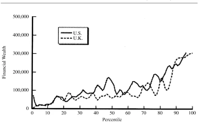
In making the right comparison across countries we need to match our datasets in a way that is robust to potential nonlinearities in the relationship between income and wealth. Therefore, the companion Figure 4 presents the same data except that now the U.K. financial wealth data are matched to U.S. household income percen-tiles, adjusted so that levels of household income are the same in both countries. For example, since median income in the United States corresponds to the 64th per-centile in the United Kingdom, Figure 4 aligns financial wealth at the 64thincome percentile in the United Kingdom with financial wealth at the median income in the United States. This is equivalent to fully nonparametric matching across percentiles of the income distribution. This figure shows that some but certainly not all of the excess financial wealth in the United States is due to income differences between the two countries, especially among the well-to-do.
Median households are only one relevant point of comparison between the two
256 The Journal of Human Resources
Figure 3
90th Percentile Financial Wealth at Income Percentiles
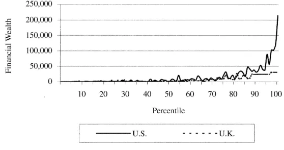
countries, Figures 3 and 5 perform the same analyses for households at the 90th percentile within each household income percentile. Here, it is much clearer that income differences between the countries cannot explain the much larger concentra-tions of wealth holdings at the very top of the distribuconcentra-tions.
To investigate changes in inequality over time, data are presented in Table 4 from the 1984 and 1994 PSID: for the United Kingdom, we append onto the 1995 BHPS series inequality measures from the 1984 and 1995 Family Expenditure Survey (FES)
Figure 4
Banks, Blundell, and Smith 257
Figure 5
90th Percentile Financial Wealth at Matched Income
in Columns 1–2.14Both countries experienced an equal increase in income inequality at the top of the distribution over this period. Since the United States is richer, and hence on what is likely to be a more concave portion of the savings income function, however, the same increase in inequality in both countries should have a larger im-pact on savings and wealth in the United States than in the United Kingdom.
After controlling for age and income, the basic differences remain. Conditional on age and income, differences in median financial assets emerge only among those over 40 and those households above median income deciles. These two factors inter-act so that among those over age 60, median financial assets are always higher in the United States. Most important, the differences between the two countries remain far greater among the richest fifth. The wealthiest top 10 percent of American house-holds within age and income cells have far more financial wealth than do the top 10 percent of British households.
VII. The Role of the Stock Market
One explanation for the substantial mid-1990s differences in finan-cial wealth holdings (espefinan-cially at the top) between the United Kingdom and United States is that they reflect smaller longer term behavioral differences exacerbated by macroshocks affecting financial holdings in both countries. An example of a mac-roshock involves the stock market surge in both countries during this period. The
258 The Journal of Human Resources
Figure 6
Time Series of Stock Prices
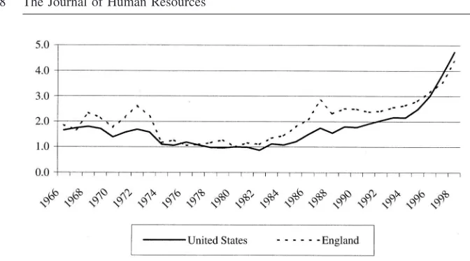
sharp appreciation in equity values may have affected financial wealth holdings dif-ferentially if households in the United Kingdom and United States differed in the initial size of their stock portfolios or if the magnitude of equity appreciation differed Figure 6 addresses the second issue by plotting inflation adjusted equity price indexes for both countries, each expressed relative to a 1980 base.15The magnitude of the recent stock market boom is impressive even compared to historical equity premiums. Real equity prices in the United Kingdom are about two and one-half times larger in real terms in 1995 as they were in 1980—slightly larger than the equity appreciation in the United States over the same period. Yet, measured from this 1980 base, it is remarkable how similar equity appreciation has been in both countries. If we instead used the mid-1970s as the reference, U.S. equity rates of return would be higher than those in the United Kingdom. This suggests that until 1980 the (recent) historical experience in the stock market was more favorable in America. Still, the compelling message from Figure 6 is that differential rates of return in each country’s equity markets during the 1980s and 1990s cannot explain the quite different levels of financial wealth holdings in each country by the mid-1990s.
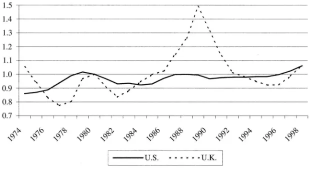
While equity appreciation was similar in the United States and United Kingdom, the relative exposure to the benefits from that appreciation were very different. In the PSID, one-quarter of U.S. households directly owned some stock in 1984, a fraction that would grow to one-third by 1994. Direct share ownership was far less common among British households especially in the early 1980s. Figure 7 plots patterns of rates of equity ownership in the United Kingdom between 1978 and 1996. By the mid-1980s, British household equity ownership rates had been stable and
Banks, Blundell, and Smith 259
Figure 7
Time Series of UK Household Share-Ownership Rates from FES Data
hovered just below 10 percent—well less than the U.S. figure in 1984. Starting in 1984, equity ownership grew more rapidly in the United Kingdom than in the United States. While the gap in equity ownership has narrowed, by the mid-1990s one-quarter of British households directly owned stock compared to one-third of Ameri-can households.
In the United Kingdom most of the increase was concentrated in a four-year period from 1985 to 1988, coinciding with the flotation of previously nationalized public utilities such as British Telecom (1984) and British Gas (1986). Around, this time,
Figure 8
260 The Journal of Human Resources
the United Kingdom government introduced also a set of measures aimed at promot-ing a ‘‘share-ownpromot-ing democracy’’—namely tax-favored employee-share ownership schemes. In the United States, the increase in share ownership was more gradual throughout the 1980s. Although the stock market boom was relatively similar across the countries, the fraction of American households benefiting was far higher than in Britain throughout the 1980s and 1990s.
Moreover, conditional on owning some stock, the value of stock holdings was considerably higher among American households. Table 5 lists values of shares owned for all households and for shareowners only as revealed in the 1995 BHPS and the 1984 and 1994 PSID. In the mid-1990s, mean value of shares in America was almost three times larger than those in Britain and about twice as large among shareholders only. In both countries, distributions of stock values are highly skewed, with concentrations in 5 to 10 percent of households. But at all points in the distribu-tions, the values of American holdings are multiples of two or three of those held by British households.
The remarkable contrast in Table 5 involves the 1995 BHPS and the 1984 PSID. Both for the full population and for shareholders only, the distribution of share values held by households is virtually identical. That is, after the stock market surge in both countries, British households had stock wealth similar to American households ten years earlier. In the early 1980s, British households’ stock holdings were consid-erably smaller than their American counterparts were. This initial condition differ-ence between the two countries would have profound impacts on wealth distributions by the mid-1990s.
That the initial share of holdings in stock market equity—the initial conditions— may have been important is demonstrated in Table 6, which lists total financial wealth obtained from the 1984, 1989, and 1994 PSID wealth modules. Since the principal differences occur at the top, the data are displayed for selected percentiles of initial wealth starting at the median. Between 1984 and 1994, there was little change in inflation-adjusted median financial wealth in the United States. Relative to roughly stable medians, these two wealth distributions became far more dispersed over these ten years. For example, in real dollars, financial wealth in the United States grew by 35 percent at the 70thpercentile and by 54 percent at the 90th percen-tile. Clearly, the 1994 American financial wealth distribution to which we are com-paring to the 1995 U.K. financial wealth distribution is a far more unequal distribu-tion than that which existed in the United States even ten years earlier.
The culprit causing rapidly increasing financial wealth inequality in the United States is easy to find. Table 7 uses 1984 deciles of household income to list changes in financial wealth alongside changes in capital gains in stocks over the same period. Since stock ownership is concentrated at the top, these data are arrayed for the 70th, 90th, and 95thpercentiles of financial wealth and changes in financial wealth respec-tively. Throughout, increments in financial net assets are almost one to one with the magnitude of the capital gains achieved in the stock market. Moreover, the largest increases in financial wealth are concentrated among the well-to-do indicating that the stock market surge was largely responsible for increasing U.S. wealth inequality during the 1980s and 1990s.16
Banks,
Blundell,
and
Smith
261
Table 5
Value of stocks and shares, by percentile of Wealth Held in Stocks and Shares, 1995 US$, thousands
1995 BHPS 1984 PSID 1994 PSID
Percentile All Share owners only All Share owners only All Share owners only
50 0.0 10.1 0.0 9.9 0.0 20.5
70 0.0 31.1 0.0 21.3 2.0 51.1
90 15.5 116.4 14.2 99.3 51.1 204.5
95 50.5 156.8 42.6 141.9 139.9 306.7
98 116.4 326.0 127.7 354.8 306.7 511.2
262 The Journal of Human Resources
Table 6
Net Financial Wealth Over Time, by Percentile of Financial Wealth, 1995 US$, thousands
BHPS PSID
1995 1995
1984 1989 1994 Lower Upper
Percentile of Financial Wealth
50 3.1 4.0 4.1 1.5 2.3
70 16.0 22.6 22.6 9.3 12.4
90 82.3 101.3 141.1 54.3 72.2
95 146.2 178.8 249.2 100.9 139.7
98 276.7 359.6 465.2 184.0 251.1
Table 7
Changes in Financial Assets and Capital Gains in Stocks, by 1984 Income Decile and Percentile of Financial Assets
Change in Financial Assets Capital Gains in Stocks Income
Decile 70th 90th 95th 70th 90th 95th
1 0.9 17.4 82.6 0.0 22.4 62.3
2 1.4 30.1 86.0 2.1 55.3 83.1
3 2.8 38.9 60.5 0.0 27.1 53.0
4 6.4 48.6 94.3 4.2 58.7 137.8
5 11.5 77.0 130.4 6.0 48.1 143.5
6 16.5 59.1 103.9 6.8 67.3 140.2
7 31.8 98.6 167.9 23.3 105.0 200.5
8 41.3 125.7 218.0 29.8 143.1 276.0
9 68.4 166.6 307.9 56.2 200.4 367.4
10 191.7 560.4 848.9 106.0 473.4 900.3
Due to limitations on availability of wealth data for earlier periods, the shape of the financial wealth distribution in the United Kingdom ten years before is more uncertain. The only microdata available covering even part of this period is the Fi-nancial Research Survey, collected privately by NOP FiFi-nancial. This cross-sectional survey was first collected over the period April 1987 to March 1988, and then on an ongoing basis, with a different design, from 1994–95 onward.17There are several
Banks, Blundell, and Smith 263
Table 8
U.K. individual Net Financial Wealth Over Time, by Percentile Individual Financial Wealth, 1995 US$, thousands
Percentile 1987–88 NOP 1995 BHPS 1997–98 NOP
50th 0.8 0.7 1.1
70th 3.4 3.5 5.0
75th 4.1 5.5 6.6
90th 17.0 24.0 24.6
95th 25.2 47.5 47.3
98th 47.1 90.0 99.1
Mean 5.9 9.9 10.3
issues in using this NOP data to understand changes in wealth distributions, the most important of which is that the NOP relates to a sample of individuals as opposed to all individuals in a sample of households. Hence, no estimate of the wealth distri-bution can be made at the household level.18
To look at changes in wealth over time therefore, Table 8 shows percentiles of the wealth distribution at the individual level in the 1987–88 NOP data and at the individual level in the 1995 BHPS data.19We present estimates from the 1997–98 NOP data to examine comparability between the two data sources. The NOP collects asset values within fixed bands and we use a simple estimate of percentiles that takes asset values to be the midpoint of bands. The 1995 BHPS and 1997–98 NOP prove to be highly consistent, with estimates for all percentiles rising slightly between the two surveys—encouraging since some households in the two surveys are separated by a time period of 18 months. Given this seeming compatibility of our two data sources, we can look at growth in percentiles from 1987–88 to1995 across the two surveys with some confidence. Strikingly, the bottom three quarters of the distribu-tion of net financial wealth remains close to constant in real terms over this period in contrast to the United States where this is true only for the bottom half. Indeed the substantial real increases in financial assets over this period are only at the 90th or even 95thpercentiles and above.
Given that stock ownership in 1987–88 was lower in the United Kingdom than in the United States, and concentrated further up the income and wealth distributions, the lack of growth in financial wealth in the middle of the distribution could be a direct consequence of the differences in initial conditions. To examine this, Table 9 lists percentiles of stock wealth conditional on being a stockholder in 1987–88 and 1995. The table shows marked rises in all percentiles at and above the median,
264 The Journal of Human Resources
Table 9
Percentiles of Individual Stock Wealth, Stockholders Only, 1995 US$, thousands
Percentile 1987–88 NOP 1995 BHPS
10 0.6 0.8
50 1.7 7.8
70 3.4 18.6
90 23.5 77.6
95 50.7 124.2
98 134.5 214.7
Mean 10.4 31.7
in accordance with the receipt of the substantial capital gains shown in the FTSE all share return index in Figure 7.20But these real gains were concentrated in far fewer hands than in the United States, suggesting that the fact that less households were in the stock market to experience these real gains is one reason why the top of the U.S. wealth distribution is now so much higher than its United Kingdom counterpart. The interaction between the initial share of stock market equity and the subsequent macroeconomic shock in equity prices during the late 1980s and 1990s is therefore an important component explaining the differences in wealth between the United States and the United Kingdom.
A. Cross-Country Differences across Equity Markets
The previous analysis shows that stock market participation has always been higher in the United States than in the United Kingdom. This has led to a difference in initial conditions that is interesting to explore. One possible explanation is that market conditions—in particular transaction costs, taxes or information—differ across the two countries. Certainly prior to the mid-1980s in Britain there was a tax bias away from direct holdings of equity toward wealth held in housing or occupational sions, since equity was more heavily taxed than consumption, and housing and pen-sions benefited from tax advantages relative to consumption. Given the structure of the tax system these differences were significantly greater in times of high inflation.21
20. One must be careful in interpreting these changes since we are using two cross-sections as opposed to a panel, and so changes are not for the same person over time. If anything these will be a lower bound on the changes experienced by the percentiles of the 1987–99 distribution, given that it is extremely un-likely that new entrants to the set of shareowners are more wealthy than those who held shares in 1987– 88.
Banks, Blundell, and Smith 265
The introduction of Personal Equity Plans and Employee Share Ownership schemes meant that, from 1987 at least, equity could be held in a more favorably taxed manner by British households. Indeed, Personal Equity Plans give holdings of equity an identical tax treatment to IRAs or 401(k)s; that is, neutral with respect to consumption. On direct holdings of equity or mutual funds held outside of PEPs or IRAs the tax treatment is also comparable across the United States and United Kingdom. Dividend income is taxed as income in both countries, and realized capital gains are taxable in both countries. In the United Kingdom, however, capital gains are taxed only above a fairly sizable annual exemption (around $10,000 per year) whereas in the United States, capital gains are taxed at a rate lower than that in the United Kingdom (and also varying with the length of the time the asset is held) but with no exemption.
Perhaps a more pertinent difference is stamp duty, where a 0.5 percent charge is levied on all share transactions in the United Kingdom. But for infrequently traded portfolios, this difference is unlikely to be behind the marked differences in share ownership observed across the two countries. Finally, there could be differences in the information individuals have about stock market investment opportunities. Although this is a plausible explanation for differences in the middle of the income distribution, the previous analysis shows that there are cross-country differences even in the very highest percentiles of the income or wealth distribution, where such information differences are unlikely to be so pronounced.
Another explanation far these differences, and possibly for higher accumulations of financial wealth in America compared to most of Europe (including the United Kingdom) more generally, involves differences in attitudes toward capitalist financial institutions. Especially during the 1970s and early 1980s, it is probably a fair charac-terization that there was more distrust of the fairness of capitalism as an economic system at least among significant segments of the European population. The stock market is one of most vivid capitalist symbols so this distrust may have resulted in lower average participation in equity markets among Europeans. This could be one reason why the equity boom that eventually occurred in the United Kingdom affected fewer households.
The existence and importance of ideological differences are always difficult to test, especially among economists who tend to be wary of them. The approach used here compares financial wealth portfolios of U.K. citizens who self-identify with either the Labour or Conservative Party.22 Especially during the 1970s and early 1980s, it may also be a fair characterization that distrust of the fairness of capitalism was stronger among those who self-identified with Labour. Since Conservative and Labour supporters differ in other salient ways (particularly age and income) that might affect wealth holdings, it will be necessary to control for such factors.
Table 10 documents differences between the parties in their participation in equity markets. One-third of Conservative affiliates held stock compared to about one-fifth of Labour affiliates. Among those who held some stock, mean value of those holdings
266 The Journal of Human Resources
Table 10
Share Ownership and Political Preferences in the United Kingdom, Values: 1995 US$, thousands
Conservative Labour Unaffiliated (22.9 percent) (36.3 percent) (40.8 percent)
Descriptive statistics
Proportion with shares 0.346 0.209 0.208
Mean share wealth (shareholders only) 69.1 32.5 30.7 Median share wealth (shareholders only) 23.3 7.8 7.8 90thpercentile share wealth (shareholders only) 170.8 62.1 79.2
Regression coefficients
Financial wealth 17,926.01 ⫺5,070.12
t-ratio 5.559 ⫺1.845
Probability of owning shares (marginal effect) 0.056 0.006
t-ratio 3.25 0.42
Proportion of financial wealth held in shares 0.056 0.006
t-ratio 4.357 0.509
Note: All regressions control for age and education of head of household as well as for household income decile. Probit for being a shareholder and regression on proportion of financial wealth held in shares also control for level of financial wealth.
was about $69,000 for Conservatives and $33,000 for Labour. The differences at the 90thpercentile are more striking. To see if such differences could be explained by differing attributes of affiliates of these political parties we estimated a set of models controlling for income decile, our three broad age groups, and education of the household head.
Table 10 also reports estimated parameters on these political group variables, where the base case is an unaffiliated head of household. The first line of coefficients reported come from a linear regression for financial wealth conditioning on age, education, and income, and show that Conservative households are more likely to have accumulated wealth. Therefore, we condition on the level of financial wealth in what follows. In the second line of coefficients we run a probit for share ownership, which indicate that, even conditional on income, age, education, and financial wealth, Conservative supporters are 5 percentage points more likely to be share holders than their Labour counterparts. Finally, we look at the proportion of financial wealth held in shares (for those with positive financial wealth) and show that, again conditional on income, age, education, and level of financial wealth, a Conservative supporter would hold around 4 percent more of their wealth in shares than an equivalent Labour supporter.
Banks, Blundell, and Smith 267
differences that existed between the United Kingdom and United States especially in the late 1970s and early 1980s.
This analysis has shown that differences in the holdings of stock market equity in the early 1980s that predate the stock market boom are an important component of the changes in wealth inequality in recent years. But these initial differences do not explain everything. That is, there are apparently some behavioral differences between households in these two countries that produce far smaller financial wealth holdings of British households compared to American households. We deal with this important issue below.
VIII. Motives for Financial Wealth Accumulation
Initial conditions cannot explain all differences in financial wealth between British and American households. As they age, and especially during their post-retirement ages, even the median American households appear to have accumu-lated significantly more financial wealth than British households were able to do. This disparity grows much larger in the top fifth of wealth holders in both countries. In subsequent sections, we discuss some theoretical reasons for these differences. The data have suggested that the following facts need to be explained. First, for median households, except for the very highest income deciles, at young ages there appears to be very little difference in financial wealth holdings between U.S. and U.K. households. In fact, young households in both countries have few financial assets of any kind. As households age and incomes grow over the life cycle, a sig-nificant gap in median financial assets emerges until after age 60 the gap in financial assets is substantial even for the median household. Second, for those 10 to 20 per-cent of households at the top (say the 90thpercentile), there is a substantial disparity in financial wealth holdings between the U.K. and U.S. households even at young ages. This gap has an even more pronounced age and income gradient until at older ages the difference in financial wealth holdings between the wealthiest U.S. and U.K. households is very, very large indeed.
Economic theory suggests several potentially important motives for wealth accu-mulation, including an altruistic bequest motive to bequeath financial resources to one’s heirs, precautionary savings motives to reduce risks associated with income, health, or longevity, and smoothing life-cycle timing of consumption and income paths. There may also be institutional and historical differences between the countries that lead to American and British households selecting quite different portfolios of financial and other assets. We organize our discussion in this section around these motives.
A. Precautionary Motives
268 The Journal of Human Resources
health conditions, or longevity will tend to increase current savings and, at least in earlier part of the life cycle, consumption will tend to follow income.23The basic question here is whether older American households face more age-related risks than their British counterparts do.
1. Income Risk
A key financial risk faced by households is that associated with fluctuating incomes during their working lifetimes. As such, one would expect income risk to be an important factor in determining precautionary balances of liquid and semi-liquid financial assets.24 One can think of overall income risk as being determined by a number of subcomponents, namely income risk conditional on remaining in employ-ment, employment risk itself, and then the duration of, and associated financial con-sequences of, spells out of the labor market following labor market separations. If one considers household incomes as the concept of interest, there are also issues related to the magnitude of these three components for each adult household member, and this also introduces a fourth component—the risk of household separation itself. Indeed, one could define income as income relative to needs in which case the risk of household formation and separation, as well as child bearing, will have clear financial consequences for household ‘‘incomes.’’
Yet, it is also important to distinguish between true risk and simple fluctuations over time. Many changes may be anticipated by household members and ought not to be considered as determinants of precautionary saving. Obviously, the availability of a long series of panel data is a crucial instrument in extracting the risk component from time series variations and to do so for both countries in this study on a compara-ble basis is an interesting and important agenda.25 At this stage, however, we are content to point out that many of our observed differences in financial wealth are most pronounced amongst late middle age and even the retired age groups where such income risks might be thought to be predominantly resolved. Income risks for those cohorts will undoubtedly have played a role in generating the wealth each cohort has accumulated by the mid-1990s but we think it unlikely that cross-country differences in employment or income risk can be large enough to have been a major influence for these older age groups.
When one looks at needs, the conclusion does not change substantially. Family compositions are comparable in the United States and the United Kingdom, and one would expect the relative financial implications of unexpected changes in household size to be comparable also. Similarly, the concentration of the largest disparities
23. In a variant of this model, impatience for the present duels with prudence as individuals maintain a ‘‘buffer stock’’ of a small amount of wealth to deal with future uncertainty. The buffer stock remains small due to impatience. Another avenue explored in recent work involves liquidity constraints—that individuals cannot borrow and lend at the same interest rate. With liquidity constraints, individuals will not be able to borrow as much to finance their current consumption, and consumption will follow income more closely.
24. See Banks, Blundell, and Brugiavini (2001) for an empirical demonstration of this in the United King-dom, or Hubbard, Skinner, and Zeldes (1994) for a U.S. example.
Banks, Blundell, and Smith 269
among the oldest age groups suggests that savings for children’s college education expenses, which will tend to be larger in the United States, seem an unlikely explana-tion of these differences. If wealth accumulaexplana-tion for educaexplana-tion expenses were the principal explanation, then we should observe wealth differences between the coun-tries narrowing after the point in the life cycle when these expenses are normally incurred. We do not observe such a narrowing.
2. Health Risk
One well-known difference in institutional structure between the United States and United Kingdom is in the provision of health care. As such, at least one risk that may differ across countries relates to the financial consequences of bad health shocks, both in working life and during retirement. Such differences are unlikely to be driv-ing such large differences in financial wealth accumulation as those observed earlier. The most important differences in health care systems are during working ages, where the United States has a predominantly private system in contrast to Britain’s universal provision. At these ages, the prevalence of private insurance in the United States shows that self-insurance is uncommon and hence average asset accumulation profiles are unlikely to be substantially affected. At older ages, health care for the elderly is universally provided in both countries, so again accumulation is unlikely to occur differentially in anticipation of adverse health events during old age.
Aside from the direct health care components, the other financial liabilities are out-of-pocket expenses and financing of long-term care needs. With regard to the former, privately borne costs have risen in Britain, as a result of the means testing of publicly paid medical, dental, and optical expenses for working-age households. Retired households, however, continue to receive completely free medical prescrip-tions, as well as not being liable for expenses associated with dental or optical care. Again, such differences are unlikely to explain such huge wealth accumulation dis-parities as are observed across the two countries. With regard to long-term care, there are similarities between the United States and Britain where care is essentially privately financed. More precisely, in Britain the care component (as opposed to the health care component) needs to be privately financed. There is a low-quality public long-term care option for those below a (low) threshold of financial assets, but such an option would typically not be relevant to even the median wealth elderly household.
3. Longevity Risk
Once retired, the intertemporal planning problem becomes one of decumulating assets at an optimal rate, enjoying the benefits of current consumption though ensuring that expected future consumption will not be too low. Even at retirement, once earnings and employment risk have been resolved, individuals still face risks since the number of time periods over which their available resources have to be spread is uncertain. Earlier than anticipated death will lead to accidental bequests, but probably more impor-tantly, an individual who lives ‘‘too long’’ could end up facing periods of very low consumption, depending on the generosity of state support for the elderly.
270 The Journal of Human Resources
(Defined Benefit) pension wealth are by definition annuitized, this is more of an issue for some households than for others. On top of this, there are differences in compulsory annuitization requirements across countries. More specifically, in the United Kingdom, individuals with a defined contribution pension scheme are forced to annuitize 75 percent of their pension fund sometime between the ages of 50 and 75.26 Only a small number of individuals currently receive income from such an
annuity. In the future, however, as a result of the 1986 Social Security Act allowing individuals to ‘‘opt out’’ of SERPS into a defined contribution pension scheme and the subsequent popularity of both Private Personal Pensions and occupational defined contribution pension plans, many more individuals will reach retirement with wealth in a form that under current rules requires annuitization. Issues such as the return provided by annuities, whether individuals should be subject to mandatory annuitiza-tion, and the design of any alternative income draw-down arrangements are important ones for today’s working-age households.
As long as arrangements remain as they currently are, it is certainly the case that U.K. individuals are less exposed to the ‘‘risk of living too long’’ than are their U.S. counterparts. Not only will public pensions provide an annuity stream but private pen-sions, which represent a growing component of household wealth for working-age households, will also provide a stream of income for as long as individuals are alive. However, the corollary of this is not necessarily a reduction in overall risk, but instead a change in the risks that an individual faces and a change of the point in time at which those risks are resolved. After all, the level of the retirement income generated from private pensions for a U.K. household will be determined by the market for annuit-ies at the time the annuity is purchased, which in turn generates its own risks.
One might argue that if insurance against longevity risk were a big issue in the United States there would presumably be a large market for voluntarily purchased annuities. Friedman and Warshawsky (1990), however, show that the observed lack of demand for annuities by young retirees can be explained by actuarially unfair pricing, which could result from transaction costs, market power or simple adverse selection in the annuity market.27This suggests that, to the extent that adverse
selec-26. The element of their pension fund which comes from the contracted-out rebate has to be converted into a ‘‘protected rights’’ annuity between the ages of 60 and 75. A protected rights annuity is one that pays the same rate for both men and women—that is, insurance firms are not allowed to offer better terms to men despite their lower life expectancy. Such rules therefore build in redistribution, on average, from men to women, from rich to poor, and from single adults to married couples.
An individual who has made additional voluntary savings into their pension fund is, on retirement, allowed to withdraw 25 percent of this as a tax-free lump sum. The remaining 75 percent of the fund must purchase a ‘‘compulsory’’ annuity between ages 50 and 75. Unlike protected rights annuities, insurance firms can offer higher annuity rates to men than women, reflecting their lower life expectancy. Individuals are given various options for how to annuitize this part of their pension savings. They may purchase annuities fixed in nominal terms, indexed to prices, escalating, or linked to some investment. Annuities can be purchased on either a single or a joint life basis. Those choosing to defer annuitization past their retirement can make annual income withdrawals of between 35 and 100 percent of an amount calculated (in Government Actuary annuity rate tables) to be that which an annuity purchased with the fund would have provided. If the individual dies before they have annuitized their fund, the remaining balance is subject to tax of 35 percent and is bequeathable. This makes the income draw-down arrangements particularly attractive to anyone with a bequest motive. For more details and evidence, see Banks and Emmerson (1999).