Succession processes in a food web of a
two autotroph – one herbivore system
Dipak Kesh *, A.K. Sarkar, A.B. Roy
Department of Mathematics,Di6ision of Biomathematics,Centre for Mathematical Biology and Ecology,Jada6pur Uni6ersity, Calcutta700 032,India
Received 17 February 2000; accepted 19 May 2000
Abstract
This paper deals with the succession process of a food web model consisting of one herbivore, two autotrophs and available nutrient in the environment in a closed nutrient flux. The model provides a way of describing successional changes in the form of species replacement with increasing nutrient levels. It is shown that distinct threshold (with upper and lower) values of nutrient are required for progression of succession process. © 2000 Elsevier Science Ireland Ltd. All rights reserved.
Keywords:Succession; Nutrient flux; Saturated equilibria; Uniform persistence
www.elsevier.com/locate/biosystems
1. Introduction
Ecosystem changes may be caused by fluctua-tions in the internal population interacfluctua-tions or by fluctuations of the controlling factors. Such changes could be cyclical changes or directional changes from less complex to more complex com-munities, and can be considered as progression in succession. During progressive succession there is usually an increase in productivity of biomass, related to stability and diversity of species. Suc-cession is a typical example of an irreversible process in ecology in which co-operation between
organisms replace one another in a given region. The succession of species population may be a result of one or a combination of general factors: (i) phenotypic characteristics of species (some en-tering a disturbed area sooner than others and growing faster); (ii) externally imposed changes in one or more environmental parameters that fa-vour some species over the others; (iii) changes in the environment caused by the populations them-selves (see DeAngelis, 1992; Smith, 1990).
In this paper a possible succession process due to changes in the amount of nutrients will be analysed on the assumption that succession ends in the formation of a stable climateric biocenosis. Rosenzweig (1971) studied a series of predator-prey models with different predator-prey productivities and predator functional response curves, and estab-lished the possibility of oscillatory instability un-* Corresponding author. Tel.:+91-33-4720717; fax:+
91-33-4720964.
E-mail address:[email protected] (D. Kesh).
der conditions of nutrient enrichment. Armstrong (1979) modelled the process of succession under gradual changes in environmental conditions, namely, increases in nutrient levels in the ecosys-tem, or ‘eutrophication’ to one-prey many-preda-tor systems. He described a graphical approach in order to analyse succession changes along gradi-ents of nutrient enrichment. Alekseev (1982) also discussed a model of Lotka – Volterra type in or-der to study succession and predicated simple and complex succession series obtained from the sta-bility conditions of possible stationary states at different levels of total nutrients. Holt et al. (1994) studied a food-web model and assumed that the model is closed with respect to the limiting nutri-ents. It is found in their study that distinct thresholds of nutrient levels are required to sup-port the various food-web configurations. Re-cently, Kesh et al. (1997) studied succession in a three species food chain model and found that distinct thresholds of nutrient levels are required to support the species of the food chain.
The succession process through species replace-ment with increasing nutrient level changes in autotroph species composition under temporal or spatial gradients in nutrient levels has been ob-served in many studies. Olsen and Willen (1980) reported on the effects of reduction in phospho-rous loading to Lake Vattern in Sweden and subsequent changes in phytoplankton volume in the lake during a period of ten years. DeNoylles and O’Brien (1978) enriched experimental ponds with nitrogen, phosphorous and potassium in or-der to study phytoplankton succession. Davy and Bishop (1984) also investigated the effects of addi-tion of nutrients to a Breckland grass heath. It was observed that nutrient addition caused an increase in the biomass of Festuca o6ina and
Koeleria macrantha, whereas the biomass of com-peting species such asHieracium pilosella showed a considerable decline. DeAngelis (1992) discussed species replacement with increasing nutrient levels in an environment closed to nutrient flux.
In this paper, possible succession process as due to changes in the amount of nutrients will be analysed under the assumption that succession ends in the formation of a stable climateric bio-cenosis. We investigate the succession series of a
food-web model comprising two autotrophs com-peting for a single limiting resource and grazed on by a single generalized herbivore. In the proposed model the growth of autotrophs are assumed to follow Lotka – Volterra type interactions with the available nutrients while the uptake rates of the generalized predator are taken in a general func-tional form. From the model study it appears that the co-existence of one autotroph with a corre-sponding herbivore depends on the upper and lower threshold levels of available nutrients and also on the form of the uptake function of the herbivore. If threshold levels of nutrients are fur-ther enhanced, co-existence of two autotrophs and one herbivore is possible provided an intricate relationship between uptake functions of the first and second autotroph by the herbivore is satisfied. From the model study it appears that both au-totrophs can not co-exist in the absence of the herbivore.
The organisation of the paper is as follows. In Section 2, a food-web model and mathematical preliminaries are presented. Section 3 deals with the existence of possible boundary equilibria. In Section 4, stability conditions and possible simple and complex succession series for the model are discussed. A numerical example is given in Section 5 to illustrate the results. Lastly, a discussion follows in Section 6.
2. The model and basic results
We consider here a trophic scheme of a food-web comprising two autotrophs and one herbi-vore with nutrient limited growth in a closed environment, whose total nutrient level N in the environment is assumed to be conserved. Let
x1(t),x2(t) andy(t) denote equivalent biomass (or
the mass of the limiting nutrient) of autotrophs and herbivore respectively and Ro(t) be the mass
of the available limiting biogenic resources (nutri-ent) in the environment.
dx1
dt = −o1x1−y p1(x1)+b1x1Ro (2.1)
dx2
dt = −o2x2−y p2(x2)+b2x2Ro
dy
dt= −o3y+y(p1(x1)+p2(x2))
dR0
dt =o1x1+o2x2+o3y−Ro(b1x1+b2x2)
with xi(0)=xi0\0,i=1, 2 andy(0)=y0\0.
Here the uptake rates of available nutrients by autotrophs are taken in Lotka – Volterra form while response function of the generalized herbivore is taken in a general formpi(xi);i=1, 2. Also o1,o2,
o3 are the mortality rates and b1, b2 are the
efficiency rate of utilizing the resources, which are taken to be positive.
From the (Eq. (2.1)) it follows that
Ro(t)+x1(t)+x2(t)+y(t)=Constant=N (say)
(2.2)
Hence the model meets the conservation princi-ple.Using conservation condition (Eq. (2.2)) for nutrient in (Eq. (2.1)), we get the following system as:
dx1
dt =b1x1(N−l1−x1)−b1x2x1
−y(p1(x1)+b1x1)
dx2
dt =b2x2(N−l2−x2)
−b2x1x2−y(p2(x2)+b2x2) (2.3)
dR0
dt =y(−o3+p1(x1)+p2(x2))
where li=oi/bi; i=1,2.
In this systemRois not explicitly present and it
resembles a two autotroph – herbivore system in which autotrophs are in competition, and the functional response of the herbivore is enhanced to the form pi(xi)+bixi.
2.1. Remark 1
From the model (Eq. (2.3)) it seems that there is indirect vertical interactions among the autotroph – herbivore levels and indirect horizontal
(competi-tive) interactions. These indirect effects are mediated through direct interactions in a food-web of herbivores that share two autotroph in an environment which is closed with respect to limiting nutrients.
2.2. Hypotheses
We impose the following hypotheses on the functions pi (for interpretation of (a) and (b) see
Freedman, 1980) in order to analyze the model.
(H1)
(a) pi: R+R, and these are C
1functions.
(b) pi(0)=0; p%i (xi)\0 forxiR+and
lim
xi
pi(xi)=piB+
(c) pi(xi)Bo3 forxi(0 mi);
pi(xi)\o3 forxi(mi,N−li)
where (N−li) is the carrying capacity of
au-totrophsxiandmirepresents the threshold value (or
breakeven concentration) of xi below which the
herbivore can not grow and above which (but less thanN−li) the specific growth rate ofyis positive.
(d) d dxi
pi(xi)xi
B0 forxi(0, N−li)(e) l1 is less thanl2.
2.3. Lemma 2.1
All solutions of system (2.3) that initiate in R+3
for all initial points (x10, x20, yo) are eventually
uniformly bounded and enter into a region B defined by
B={(x1,x2,y)R+
3 : 0Bx
iBCi;
0Bx1+x2Bk2/m1;
0Bx1+x2+yBk2/m2} (2.4)
where
Ci=N−li,k2=C1g1(0)+C2g2(0)+h1+h2
m1=min[g1(0), g2(0)],m2=min[g1(0), g2(0),o3]
2.4. Proof
By assumption (H1), both of the autotrophs are limited by their carrying capacities, and so from (Eq. (2.3))
x;i5xibi(N−li−xi)=xigi(xi);i=1, 2.
By the usual comparison theorem (Hale, 1969), we have
xiBCi=N−li
Let us define, S1(t)=x1(t)+x2(t). The time
derivative along a solution of the system is
S: =x1g1(x1)+x2g2(x2)−(b1+b2)x1x2
−y(p1(x1)+b1x1)−y(p2(x2)+b2x2)
5x1g1(x1)+x2g2(x2)
= −(x1g1(0)+x2g2(0))+x1g1(0)+x2g2(0)
+x1g1(x1)+x2g2(x2)
or,
S:5−m1(x1+x2)+C1g1(0)+C2g2(0)+h1+h2
Therefore,
S:1+m1S1Bk2, wherek2
=C1g1(0)+C2g2(0)+h1+h2
Applying a theorem on differential inequalities (Birkhoff and Rota, 1982), we obtain
05S15(k2/m1)+e−mtS1(x1(0),x2(0)).
As t , 0BS1Bk2/m1.
Define S2(t)=x1(t)+x2(t)+y. Then
S:2=x;1+x;2+y;2
5x1g1(x1)+x2g2(x2)−o3y
= −(x1g1(0)+x2g2(0)+o3y)+x1g1(0)
+x2g2(0)+x1g1(x1)+x2g2(x2).
Therefore,
S:2B−m2(x1+x2+y)+C1g1(0)
+C2g2(0)+h1+h2,
or S:2+m2S2Bk2and 0BS2Bk2/m2 as t .
Hence system (2.3) is dissipative with the asymptotic boundk2/m2. Thus there is a compact
neighbourhood B¤R+3 such that for sufficiently
large T=T(x0,t0), x(t)B for all t\T, where
x(t)={x1(t),x2(t),y(t)} is a solution of (2.3) that
initiates in R+
3 . This completes the proof of the
lemma.
3. Existence of possible boundary equilibria
In system (2.3), when all species are absent, the trivial equilibrium E0(0,0,0) always exists. The
existence of other boundary equilibria depends critically on the amount of total nutrient Nin the environment. The axial equilibria E1(N−l1, 0, 0)
and E2(N−l2, 0, 0) exist provided N\l1 and
N\l2, respectively. We now investigate the
inte-rior equilibrium in the positive x1−y plane.Here
isoclines are x;1=0, or y=F1(x1; N)where
F1(x1;N)=
b1(N−l1−x1)
p1(x1)/x1+b1
(3.1)
and y; =0 is the vertical line x1=m1, where m1 is
finite.
From (Eq. (3.1)), F1(N−l1; N)=0 and
F1 (0;N)=limF1(x1;N)=
b%(N−l1)
p%1(0)+b1\0
dF1(0;N)
dx1
= lim
x10+
F1(x1;N)
= −2b1(p%1(0)+b1)+b1(N−l1)p¦(0) 2{p%1(0)+b1}
2
a possible configuration of the autotroph isoclines is given in Fig. 1.
Hence the unique interior equilibrium
E13
m1,0,b1(N−l1−m1)
p1(m1)/m1+b1
exists in the x1−y plane provided
Fig. 1.
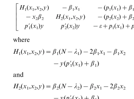
Æ Ã Ã Ã È
H1(x1,x2,y) −b1x1 −(p1(x1)+b1x1)
−x2b2 H2(x1,x2,y) −(p2(x2)+b2x2)
p%
1(x1)y p%2(x2)y −o+p1(x1)+p2(x2)
Ç Ã Ã Ã É
where
H1(x1,x2,y)=b1(N−l1)−2b1x1−b1x2
−y(p%1(x1)+b1) and
H2(x1,x2,y)=b2(N−l2)−b2x1−2b2x2
−y(p%2(x2)+b2). (4.1) EvaluatingVat different equilibria, we get their local stability properties.
4.1. Case 4.1: NBl1Bl2
Eo is a sink (i.e. Eois saturated). No organism
can live in the environment.
4.2. Case 4.2: l1BNBl2
E0 and E1 exists and no other boundary
equi-libria are feasible. E0 is a hyperbolic saddle point
(or equivalently non-saturated). It has along each of they-axis andx2-axis a non-empty one
dimen-sional (local) stable manifold.
The flows along the x1 and x2 axes are away
fromE0and approachE1.E1is stable or unstable
(locally) along they-direction according as −o3+
p1(N−l1)B or \0, i.e.NB or \l1+m1. SoE1
is unstable along y-direction and y always in-creases (as its invasion parameter −o3+p1(N−
l1)\0) at the axial equilibrium E1 ifN\l1+m1.
Hence E1 becomes a saturated equilibrium for
l1BNBl1+m1Bl2 (4.2)
E1 becomes non-saturated for
l1Bl1+m1BNBl2. (4.3)
We now have the following result.
4.3. Theorem 4.1
Suppose that l1BNBl1+m1Bl2. Then any
solution of system (2.3) with xi(0)\0, y(0)\0
satisfies Similarly, under (H1)
E23
0,m2,b2(N−l2−m2)
p2(m2)/m2+b2
exists inx2−y plane provided
N\l2+m2. (3.3)
From (Eq. (2.3)), it follows that if the herbivore is absent, two autotrophs can not attain
E12(x1,x2,0) and they are in a dominance state.
Existence of different axial and planar equi-libria thus depends critically on the total nutrient
N, li andmi; i=1,2.
It is difficult to determine the interior equi-librium E*(x*1,x*2,y*) but one can gain
informa-tion about whether the two autotrophs and the herbivore can co-exist or not.
4. Stability of equilibria
We denote by V+(E) and V−(E) as the local
stable and unstable manifolds respectively, of equilibrium E. Let xR+3 , and let V(x) be the omega-limit set of the orbit through x.
Local stability properties of the feasible boundary equilibria are obtained by computing the variational matrixV(x) of system (2.3) about these equilibria. The variational matrix of (Eq. (2.3)) is given by
limx1(t)=N−l1,
Under the assumption of Theorem 4.1, it fol-lows thatE1is a saturated equilibrium. Thus it is
a local attractor and autotrophx2cannot survive
since x;B0 for NBl2. Hence by the Butler –
McGehee lemma (Freedman and Waltman, 1984) it follows thatE0is not the v-limit set and hence
all orbits with positive initial condition converge to the equilibrium E1. From the conservation
condition (2.2), it also follows that
limR0(t)l1
t
4.5. Case4.3:l1+m1Bl2BNBl2+m2
Under this assumption, E0, E1, E2, E13 are
possible boundary equilibria. From the varia-tional matrix, E0 is non-saturated. It has along
each of the xi-axes a non-empty one-dimensional
(local) unstable manifold. The flows along the x1
and x2-axes are away from E0 and approach E1
and E2, respectively. E1 is unstable along the
y-directions sinceN\l1+m1. WhenNBl2+m2,
E2has a non-empty one-dimensional (local) stable
manifold in the x2–y plane. Hence E2 is
non-saturated.
The variational matrix at (E13) is
V(E13)=
All eigenvalues are negative or have negative real parts if
We next show that E13 is a global attractor in
x1−y plane. From (3.2) we have,
be any periodic orbit aroundE13 in x1−y plane.
Hence DB0. So, by the Poincare Bendixson theorem (Conway and Smoller, 1986) any periodic orbit is stable. HoweverE13is locally stable in the
x1−y plane, a contradiction. Hence under (4.6)
and (4.7), there is no periodic orbit aroundE13in
the positive x1−y plane.
4.6. Remark 2
Let the isocline of autotrophx1and the isocline
of herbivore y intersect at E(m1,y) (see Fig. 1)
whereHmByBHM;HmandHMbeing the global
minimum and global maximum values ofF1x1(x1;
N). Now we have following two possibilities: 1. If a22B0, a11\0, one eigenvalue is positive
and two are negative. Hence E13 is locally
unstable inx1−yplane but stable along thex2
direction.
2. If a22\0, a11B0, then also E13 is locally
stable in x1−y plane and unstable along the
x2 direction.
unstable in x1−y plane. Hence by the Poincare –
Bendixson theorem (Conway and Smoller, 1986) there may exist at least one limit cycle aroundE13.
If N=l1+m1+(m1/(1−M1)), then the real part
of the eigenvalues of E13 become zero and there
exists Hopf-bifurcating small amplitude periodic solutions around E13.
In ( 2 )a22\0, a11B0[l1+m1+
Therefore,E13is a global attractor under
condi-tions (4.7) and its invasion parameter is negative for all t\0. Since the system (2.3) is dissipative (by Lemma 2.1), we get the following result.
4.7. Theorem 4.2
Let (H1), Lemma 2.1 and conditions (4.7) hold. Then boundary equilibrium E13 attracts all
solu-tions of (2.3) with x2(0)\0, that is
exist. We shall now investigate the conditions for uniform persistence of the system (2.3). To derive conditions for uniform persistence of the system, we need other assumptions, namely
(H2) There exist no periodic orbit on x1–y plane
and x2–y plane for the system (2.3).
Let us consider an average Lyapunov function of the form (see Hofbauer, 1981; Hutson and Vickers, 1983).
E13 is globally asymptotically stable in x1−y
plane by conditions (4.7), and there is no periodic solutions around it. Hence by (H1), (H2) and (H3), thev-limit set of every orbit on boundary B consists of fixed points. So uniform persistence of the system (2.3) holds ifcis positive atE0,E1,E2,
Let (H1), (H2), (H3), Lemma 2.1 and condi-tions (4.7) hold, and if
1. b2 then the system (2.3) is uniformly persistent.
4.10. Remark 3
If we reverse the condition of H1(e), then we get similar results by changing the suffix of all previous results as discussed from Case 4.1 to 4.4.
It is easy to see that all the hypothesis of (H1) are satisfied. All solutions of (5.1) which initiate in
R+
3 will enter the confined convex set
B defined
3 will converge to the
equi-librium (N−1/2, 0, 0) andR0=1/2 as t .
4. If N\26.458, then either of the autotrophs competiting for the same limiting nutrient will go to extinction.
6. Conclusions
Successional changes can be explained utilizing population dynamics, especially competition, re-generation, mortality and by physiology and life history strategies. Species composition over time is determined by the development and response to competition. The replacement of species by other species results in part from interspecific competi-tion which permits one group to suppress the other. Thus the succession comes about as the relative availability of resources changes through time. Community composition changes along the gradiant as the availability of limiting resources changes and the species reach an equilibrium with this availability. In doing so, they lower the avail-able resources to a point at which other species can not invade.
From the present study, it follows that if
N(l1,l1+m1) wherel1+m1Bl2then autotroph
x1 exists for all future time but no other
au-totroph and its herbivore can survive. This is the first stage of succession.
The second stage of succession involving co-ex-istence of the first autotroph x1 and its herbivore
becomes successful, provided the total nutrient N
is further enhanced and lies in the threshold
l1+m1,l1+minand the specific uptake rate for autotroph x1
satisfies the condition
In this case autotroph x2 can not grow in the
environment.
The last phase of succession in which two au-totrophs and a generalized herbivore co-exist is attained provided Nis further enhanced and lies within the threshold
This dynamics does not follow the usual succes-sion series of its states from pioneer to climax (stable), but this study does gives conditions on the resources for one to study the introduction of species to form a food chain/web.
Acknowledgements
We thank the referee for his comments regard-ing the improvement of the paper.Research sup-ported by the CSIR, Ref. No. 9/96(240)/94-EMR-I, Govt. of India and UGC-DSA (Phase-III), Department of Mathematics, Jadavpur Uni-versity, Calcutta, India.
References
Armstrong, R.A., 1979. Prey species replacement along a gradient of nutrient enrichment: a graphical approach. Ecology 60 (1), 76 – 84.
Birkhoff, G., Rota, G.C., 1982. Ordinary Differential Equa-tions. Ginn, Boston.
Conway, E.D., Smoller, J.A., 1986. Global analysis of a system of predator – prey equations. SIAM J. Appl. Math. 46, 630 – 642.
Davy, A.J., Bishop, G.F., 1984. Response of Hieracium pi-losellain Breckland grass heath to inorganic nutrients. J. Ecol. 72, 319 – 330.
DeAngelis, D.L., 1992. Dynamics of Nutrient Cycling and Food Webs. Chapman & Hall, London.
DeNoylles, F., Jr, O’Brien, W.J., 1978. Phytoplankton suc-cession in nutrient enriched experimental ponds as related to changing carbon, nitrogen and phosphorus conditions. Arch. Hydrobiol. 84, 137 – 165.
Freedman, H.I., 1980. Deterministic Mathematical Models in Population Ecology. Marcel Dekker, New York. Freedman, H.I., Waltman, P., 1984. Persistence in models of
three interacting predator – prey populations. Math.
Biosci. 68, 213 – 231.
Hale, J.K., 1969. Ordinary Differential Equations. Wiley – In-terscience, New York.
Hofbauer, J., 1981. A general cooperation theorem for hy-percycles. Monatsh. Math. 91, 233 – 240.
Holt, R.D., Grover, J.P., Tilman, D., 1994. Simple rules for interspecific dominance in systems with exploitative and apparent competition. Am. Nat. 144, 741 – 771.
Hutson, V., Vickers, G.T., 1983. A criterion for permanent coexistence of species with an application to a two prey, one predator system. Math. Biosci. 63, 253 – 269. Kesh, D., Sarkar, A.K., Roy, A.B., 1997. Succession in a
three-species food-chain model. Ecol. Model. 96, 211 – 219.
Olsen, P., Willen, E., 1980. Phytoplankton response to a sewage reduction in Vattern, a large, oligotrophic lake in Central Sweden. Arch. Hydrobiol. 89, 171 – 188.
Rosenzweig, M.L., 1971. Paradox of enrichment in competi-tive systems. Ecology 55, 183 – 187.
Smith, R.L., 1990. Ecology and Field Biology. Harper Collins, New York.
.