for Causation: A Critical
Review
Introduction
Regression models are often used to infer causation from association. For instance, Yule [79] showed – or tried to show – that welfare was a cause of poverty. Path models and structural equation models are later refinements of the technique. Besides Yule, exam-ples to be discussed here include Blau and Dun-can [12] on stratification, as well as Gibson [28] on the causes of McCarthyism. Strong assumptions are required to infer causation from association by mod-eling. The assumptions are of two kinds: (a) causal, and (b) statistical. These assumptions will be formu-lated explicitly, with the help of response schedules in hypothetical experiments. In particular, parameters and error distributions must be stable under interven-tion. That will be hard to demonstrate in observational settings. Statistical conditions (like independence) are also problematic, and latent variables create further complexities. Causal modeling with path diagrams will be the primary topic. The issues are not simple, so examining them from several perspectives may be helpful. The article ends with a review of the litera-ture and a summary.
Regression Models in Social Science
Legendre [49] and Gauss [27] developed regression to fit data on orbits of astronomical objects. The rele-vant variables were known from Newtonian mechan-ics, and so were the functional forms of the equa-tions connecting them. Measurement could be done with great precision, and much was known about the nature of errors in the measurements and in the equa-tions. Furthermore, there was ample opportunity for comparing predictions to reality. By the turn of the century, investigators were using regression on social science data where such conditions did not hold,
Reproduced from theEncyclopedia of Statistics in Behavioral Science.John Wiley & Sons, Ltd. ISBN: 0-470-86080-4.
either inside grim Victorian institutions called poor-houses or outside, according to decisions made by local authorities. Did policy choices affect the num-ber of paupers? To study this question, Yule proposed a regression equation,
Paup=a+b×Out+c×Old
+d×Pop+error. (1)
In this equation,
is percentage change over time, Paup is the number of Paupers Out is the out-relief ratioN/D,
N=number on welfare outside the poor-house,
D=number inside, Old is the population over 65, Pop is the population.
Data are from the English Censuses of 1871, 1881, and 1891. There are two ’s, one each for 1871 – 1881 and 1881 – 1891.
Relief policy was determined separately in each ‘union’, a small geographical area like a parish. At the time, there were about 600 unions, and Yule divides them into four kinds: rural, mixed, urban, metropolitan. There are 4×2=8 equations, one for each type of union and time period. Yule fits each equation to data by least squares. That is, he determinesa,b,c, andd by minimizing the sum of squared errors,
Paup−a−b×Out−c×Old
−d×Pop2.
The sum is taken over all unions of a given type in a given time period – which assumes, in essence, that coefficients are constant within each combination of geography and time. For example, consider the metropolitan unions. Fitting the equation to the data for 1871 – 1881, Yule gets
Paup=13.19+0.755Out−0.022Old
For 1881 – 1891, his equation is
Paup=1.36+0.324Out+1.37Old
−0.369Pop+error. (3)
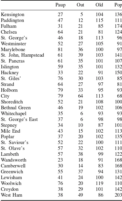
The coefficient of Out being relatively large and positive, Yule concludes that outrelief causes poverty. Table 1 has the ratio of 1881 data to 1871 data for Pauperism, Out-relief ratio, Proportion of Old, and Population. If we subtract 100 from each entry, column 1 givesPaup in equation (2). Columns 2, 3, 4 give the other variables. For Kensington (the first union in the table),
Out=5−100= −95, Old=104−100=4,
Pop=136−100=36.
The predicted value forPaup from (2) is therefore
13.19+0.755×(−95)−0.022×4
−0.322×36= −70.
The actual value forPaup is−73, so the error is−3. Other lines in the table are handled in a similar way. As noted above, coefficients were chosen to minimize the sum of the squared errors.
Quetelet [67] wanted to uncover ‘social physics’ – the laws of human behavior – by using statistical technique:
‘In giving my work the title of Social Physics, I have had no other aim than to collect, in a uniform order, the phenomena affecting man, nearly as physical science brings together the phenomena appertaining to the material world. . . .in a given state of society, resting under the influence of certain causes, regular effects are produced, which oscillate, as it were, around a fixed mean point, without undergoing any sensible alterations.’. . .
‘This study. . .has too many attractions – it is connected on too many sides with every branch of science, and all the most interesting questions in philosophy – to be long without zealous observers, who will endeavor to carry it further and further, and bring it more and more to the appearance of a science.’
Yule is using regression to infer the social physics of poverty. But this is not so easily to be done. Confounding is one issue. According to Pigou (a lead-ing welfare economist of Yule’s era), parishes with
Table 1 Pauperism, out-relief ratio, proportion of old, population. Ratio of 1881 data to 1871 data, times 100. Metropolitan Unions, England. Yule (79, Table XIX)
Paup Out Old Pop
Kensington 27 5 104 136
Paddington 47 12 115 111
Fulham 31 21 85 174
Chelsea 64 21 81 124
St. George’s 46 18 113 96
Westminster 52 27 105 91
Marylebone 81 36 100 97
St. John, Hampstead 61 39 103 141
St. Pancras 61 35 101 107
Islington 59 35 101 132
Hackney 33 22 91 150
St. Giles’ 76 30 103 85
Strand 64 27 97 81
Holborn 79 33 95 93
City 79 64 113 68
Shoreditch 52 21 108 100
Bethnal Green 46 19 102 106
Whitechapel 35 6 93 93
St. George’s East 37 6 98 98
Stepney 34 10 87 101
Mile End 43 15 102 113
Poplar 37 20 102 135
St. Saviour’s 52 22 100 111
St. Olave’s 57 32 102 110
Lambeth 57 38 99 122
Wandsworth 23 18 91 168
Camberwell 30 14 83 168
Greenwich 55 37 94 131
Lewisham 41 24 100 142
Woolwich 76 20 119 110
Croydon 38 29 101 142
West Ham 38 49 86 203
more efficient administrations were building poor-houses and reducing poverty. Efficiency of admin-istration is then a confounder, influencing both the presumed cause and its effect. Economics may be another confounder. Yule occasionally tries to con-trol for this, using the rate of population change as a proxy for economic growth. Generally, however, he pays little attention to economics. The explana-tion: ‘A good deal of time and labour was spent in making trial of this idea, but the results proved unsat-isfactory, and finally the measure was abandoned altogether. [p. 253]’
data, how can they predict the results of interventions that would change the data? The distinction between parameters and estimates runs throughout statistical theory; the discussion of response schedules, below, may sharpen the point.
There are other interpretive problems. At best, Yule has established association. Conditional on the covariates, there is a positive association between Paup and Out. Is this association causal? If so, which way do the causal arrows point? For instance, a parish may choose not to build poor-houses in response to a short-term increase in the number of paupers. Then pauperism is the cause and outrelief the effect. Likewise, the number of paupers in one area may well be affected by relief policy in neighboring areas. Such issues are not resolved by the data analysis. Instead, answers are assumeda priori. Although he was busily parceling out changes in pauperism – so much is due to changes in out-relief ratios, so much to changes in other variables, so much to random effects – Yule was aware of the difficulties. With one deft footnote (number 25), he withdrew all causal claims: ‘Strictly speaking, for “due to” read “associated with”.’
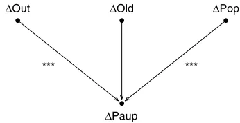
Yule’s approach is strikingly modern, except there is no causal diagram with stars indicating statisti-cal significance. Figure 1 brings him up to date. The arrow from Out to Paup indicates that Out is included in the regression equation that explains Paup. Three asterisks mark a high degree of sta-tistical significance. The idea is that a stasta-tistically significant coefficient must differ from zero. Thus, Out has a causal influence on Paup. By contrast, a coefficient that lacks statistical significance is thought to be zero. If so,Old would not exert a causal influ-ence onPaup.
The reasoning is seldom made explicit, and diffi-culties are frequently overlooked. Statistical assump-tions are needed to determine significance from the
∆Paup ∆Old
∆Out ∆Pop
*** ***
Figure 1 Yule’s model. Metropolitan unions, 1871 – 1881
data. Even if significance can be determined and the null hypothesis rejected or accepted, there is a deeper problem. To make causal inferences, it must be assumed that equations are stable under proposed interventions. Verifying such assumptions – without making the interventions – is problematic. On the other hand, if the coefficients and error terms change when variables are manipulated, the equation has only a limited utility for predicting the results of interven-tions.
Social Stratification
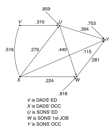
Blau and Duncan [12] are thinking about the strat-ification process in the United States. According to Marxists of the time, the United States is a highly stratified society. Status is determined by family background, and transmitted through the school sys-tem. Blau and Duncan present cross-tabs (in their Chapter 2) to show that the system is far from deter-ministic, although family background variables do influence status. The United States has a permeable social structure, with many opportunities to succeed or fail. Blau and Duncan go on to develop the path model shown in Figure 2, in order to answer ques-tions like these:
‘how and to what degree do the circumstances of birth condition subsequent status? how does status attained (whether by ascription or achievement) at one stage of the life cycle affect the prospects for a subsequent stage?’
The five variables in the diagram are father’s edu-cation and occupation, son’s eduedu-cation, son’s first job, and son’s occupation. Data come from a special supplement to the March 1962 Current Population Survey. The respondents are the sons (age 20 – 64), who answer questions about current jobs, first jobs, and parents. There are 20 000 respondents. Education is measured on a scale from 0 to 8, where 0 means no schooling, 1 means 1 – 4 years of schooling, and so forth; 8 means some postgraduate education. Occu-pation is measured on Duncan’s prestige scale from 0 to 96. The scale takes into account income, educa-tion, and raters’ opinions of job prestige. Hucksters are at the bottom of the ladder, with clergy in the middle, and judges at the top.
How is Figure 2 to be read? The diagram unpacks to three regression equations:
V
X
U
W
Y
.516
.310
.224
.279 .440 .115
.394
.281 .859
.818
.753
V is DADS’ ED X is DADS’ OCC U is SONS’ ED W is SONS’ 1st JOB Y is SONS’ OCC
Figure 2 Path model. Stratification, US, 1962
W =cU+dX+ǫ, (5)
Y =eUi+f X+gW+η. (6)
Parameters are estimated by least squares. Before regressions are run, variables are standardized to have mean 0 and variance 1. That is why no intercepts are needed, and why estimates can be computed from the correlations in Table 2.
In Figure 2, the arrow from V to U indicates a causal link, and V is entered on the right-hand side in the regression equation (4) that explains U. The path coefficient .310 next to the arrow is the estimated coefficient aˆ of V. The number .859 on the ‘free arrow’ that points into U is the estimated standard deviation of the error term δ in (4). The other arrows are interpreted in a similar way. The curved line joining V and X indicates association rather than causation:V andX influence each other
or are influenced by some common causes, not further analyzed in the diagram. The number on the curved line is just the correlation betweenVandX(Table 2). There are three equations because three variables in the diagram (U, W, Y) have arrows pointing into them.
The large standard deviations in Figure 2 show the permeability of the social structure. (Since variables are standardized, it is a little theorem that the standard deviations cannot exceed 1.) Even if father’s education and occupation are given, as well as respondent’s education and first job, the variation in status of current job is still large. As social physics, however, the diagram leaves something to be desired. Why linearity? Why are the coefficients the same for everybody? What about variables like intelligence or motivation? And where are the mothers?
The choice of variables and arrows is up to the analyst, as are the directions in which the arrows point. Of course, some choices may fit the data less well, and some may be illogical. If the graph is ‘complete’ – every pair of nodes joined by an arrow – the direction of the arrows is not constrained by the data [[22] pp. 138, 142]. Ordering the variables in time may reduce the number of options.
If we are trying to find laws of nature that are sta-ble under intervention, standardizing may be a bad idea, because estimated parameters would depend on irrelevant details of the study design (see below). Generally, the intervention idea gets muddier with standardization. Are means and standard deviations held constant even though individual values are manipulated? On the other hand, standardizing might be sensible if units are meaningful only in compara-tive terms (e.g., prestige points). Standardizing may also be helpful if the meaning of units changes over time (e.g., years of education), while correlations are stable. With descriptive statistics for one data set, it is really a matter of taste: do you like pounds, kilo-grams, or standard units? Moreover, all variables are
Table 2 Correlation matrix for variables in Blau and Duncan’s path model
Y
Sons’occ
W
Sons’1st job
U
Sons’ed
X
Dads’occ
V
Dads’ed
Y Sons’occ 1.000 .541 .596 .405 .322
W Sons’1stjob .541 1.000 .538 .417 .332
U Sons’ed .596 .538 1.000 .438 .453
X Dads’occ .405 .417 .438 1.000 .516
on the same scale after standardization, which makes it easier to compare regression coefficients.
Hooke’s Law
According to Hooke’s law, stretch is proportional to weight. If weight x is hung on a spring, the length of the spring is a+bx+ǫ, provided x is not too large. (Near the elastic limit of the spring, the physics will be more complicated.) In this equation,a andb are physical constants that depend on the spring not the weights. The parameter a is the length of the spring with no load. The parameter b is the length added to the spring by each additional unit of weight. Theǫ is random measurement error, with the usual assumptions. Experimental verification is a classroom staple.
If we were to standardize, the crucial slope param-eter would depend on the weights and the accuracy of the measurements. Let v be the variance of the weights used in the experiment, letσ2be the variance ofǫ, and let s2 be the mean square of the devia-tions from the fitted regression line. The standardized regression coefficient is
ˆ b2v ˆ b2v+s2
≈
b2v
b2v+σ2, (7)
as can be verified by examining the sample covari-ance matrix. Therefore, the standardized coefficient depends onvandσ2, which are features of our mea-surement procedure not the spring.
Hooke’s law is an example where regression is a very useful tool. But the parameter to estimate is b, the unstandardized regression coefficient. It is the unstandardized coefficient that says how the spring will respond when the load is manipulated. If a regression coefficient is stable under interventions, standardizing it is probably not a good idea, because stability gets lost in the shuffle. That is what (7) shows. Also see [4], ([11], p. 451).
Political Repression During the McCarthy
Era
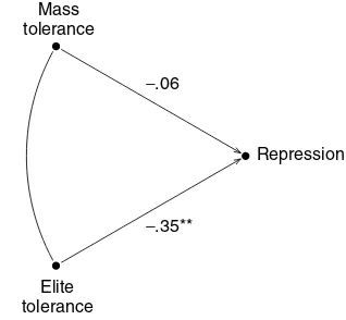
Gibson [28] tries to determine the causes of McCarthyism in the United States. Was repression due to the masses or the elites? He argues that
elite intolerance is the root cause, the chief piece of evidence being a path model (Figure 3, redrawn from the paper). The dependent variable is a measure of repressive legislation in each state. The independent variables are mean tolerance scores for each state, derived from the Stouffer survey of masses and elites. The ‘masses’ are just respondents in a probability sample of the population. ‘Elites’ include school board presidents, commanders of the American Legion, bar association presidents, labor union leaders. Data on masses were available for 36 states; on elites, for 26 states. The two straight arrows in Figure 3 represent causal links: mass and elite tolerance affect repression. The curved double-headed arrow in Figure 3 represents an association between mass and elite tolerance scores. Each one can influence the other, or both can have some common cause. The association is not analyzed in the diagram. Gibson computes correlations from the available data, then estimates a standardized regression equa-tion,
Repression=β1Mass tolerance
+β2Elite tolerance+δ. (8)
He says, ‘Generally, it seems that elites, not masses, were responsible for the repression of the era. . . .The beta for mass opinion is−.06; for elite opinion, it is −.35 (significant beyond .01)’.
The paper asks an interesting question, and the data analysis has some charm too. However, as social physics, the path model is not convincing. What hypothetical intervention is contemplated? If none,
−.06
−.35**
Repression
Elite tolerance
Mass tolerance
how are regressions going to uncover causal rela-tionships? Why are relationships among the variables supposed to be linear? Signs apart, for example, why does a unit increase in tolerance have the same effect on repression as a unit decrease? Are there other vari-ables in the system? Why are the states statistically independent? Such questions are not addressed in the paper.
McCarthy became a force in national politics around 1950. The turning point came in 1954, with public humiliation in the Army-McCarthy hear-ings. Censure by the Senate followed in 1957. Gib-son scores repressive legislation over the period 1945 – 1965, long before McCarthy mattered, and long after. The Stouffer survey was done in 1954, when the McCarthy era was ending. The timetable is puzzling.
Even if such issues are set aside, and we grant the statistical model, the difference in path coefficients fails to achieve significance. Gibson finds that βˆ1 is significant and βˆ2 is insignificant, but that does not impose much of a constraint on βˆ1− ˆβ2. (The standard error for this difference can be computed from data generously provided in the paper.) Since β1=β2is a viable hypothesis, the data are not strong enough to distinguish masses from elites.
Inferring Causation by Regression
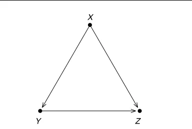
Path models are often thought to be rigorous sta-tistical engines for inferring causation from associ-ation. Statistical techniques can be rigorous, given their assumptions. But the assumptions are usually imposed on the data by the analyst. This is not a rigorous process, and it is rarely made explicit. The assumptions have a causal component as well as a statistical component. It will be easier to pro-ceed in terms of a specific example. In Figure 4, a hypothesized causal relationship betweenY andZis confounded byX. The free arrows leading intoY and Zare omitted.
The diagram describes two hypothetical experi-ments, and an observational study where the data are collected. The two experiments help to define the assumptions. Furthermore, the usual statistical analy-sis can be understood as an effort to determine what would happen under those assumptionsif the experi-ments were done. Other interpretations of the analysis are not easily to be found. The experiments will now be described.
Y Z
X
Figure 4 Path model. The relationship betweenY andZ
is confounded byX. Free arrows leading intoY andZare not shown
1. First hypothetical experiment. Treatment is app-lied to a subject, at levelx. A responseY is observed, corresponding to the level of treatment. There are two parameters,a andb, that describe the response. With no treatment, the response level for each subject will bea, up to random error. All subjects are assumed to have the same value for a. Each additional unit of treatment addsb to the response. Again,b is the same for all subjects, at all levels ofx, by assumption. Thus, if treatment is applied at levelx, the response Y is assumed to be
a+bx+random error. (9)
For Hooke’s law, x is weight and Y is length of a spring under load x. For evaluation of job training programs,x might be hours spent in training andY might be income during a follow-up period.
2. Second hypothetical experiment. In the second experiment, there are two treatments and a response variable Z. There are two treatments because there are two arrows leading into Z; the treatments are labeledX andY (Figure 4). Both treatments may be applied to a subject. There are three parameters, c, d, and e. With no treatment, the response level for each subject is taken to bec, up to random error. Each additional unit of treatment #1 addsdto the response. Likewise, each additional unit of treatment #2 addse to the response. The constancy of parameters across subjects and levels of treatment is an assumption. If the treatments are applied at levels x and y, the responseZ is assumed to be
Three parameters are needed because it takes three parameters to specify the linear relationship (10), namely, an intercept and two slopes. Random errors in (9) and (10) are assumed to be independent from subject to subject, with a distribution that is constant across subjects; expectations are zero and variances are finite. The errors in (9) are assumed to be independent of the errors in (10).
The observational study. When using the path model in Figure 4 to analyze data from an obser-vational study, we assume that levels for the variable X are independent of the random errors in the two hypothetical experiments (‘exogeneity’). In effect, we pretend that Nature randomized subjects to levels of X for us, which obviates the need for experimental manipulation. The exogeneity of X has a graphical representation: arrows come out ofX, but no arrows lead intoX.
We take the descriptions of the two experiments, including the assumptions about the response sched-ules and the random errors, as background informa-tion. In particular, we take it that Nature generatesY as if by substituting X into (9). Nature proceeds to generateZas if by substitutingXandY – the same Y that has just been generated fromX– into (10). In short, (9) and (10) are assumed to be the causal mech-anisms that generate the observational data, namely, X, Y, and Z for each subject. The system is ‘recur-sive’, in the sense that output from (9) is used as input to (10) but there is no feedback from (9) to (8). Under these assumptions, the parametersa,bcan be estimated by regression ofY onX. Likewise, c, d,e can be estimated by regression ofZ on X and Y. Moreover, these regression estimates have legiti-mate causal interpretations. This is because causation is built into the background assumptions, via the response schedules (9) and (10). If causation were not assumed, causation would not be demonstrated by running the regressions.
One point of running the regressions is usually to separate out direct and indirect effects of X on Z. The direct effect is d in (10). If X is increased by one unit withY held fast, thenZ is expected to go up byd units. But this is shorthand for the assumed mechanism in the second experiment. Without the thought experiments described by (9) and (10), how can Y be held constant when X is manipulated? At a more basic level, how would manipulation get into the picture?
Another path-analytic objective is to determine the effecteofY onZ. IfY is increased by one unit with Xheld fast, thenZis expected to go up byeunits. (If e=0, then manipulatingY would not affectZ, andY does not causeZ after all.) Again, the interpretation depends on the thought experiments. Otherwise, how couldY be manipulated andX held fast?
To state the model more carefully, we would index the subjects by a subscripti in the range from 1 to n, the number of subjects. In this notation,Xi is the value of X for subject i. Similarly, Yi and Zi are the values of Y and Z for subject i. The level of treatment #1 is denoted byx, andYi,x is the response for variable Y if treatment at level x is applied to subjecti. Similarly,Zi,x,yis the response for variable Zif treatment #1 at levelxand treatment #2 at level yare applied to subjecti. The response schedules are to be interpreted causally:
• Yi,x is whatYi would be if Xi were set to x by intervention.
• Zi,x,y is whatZiwould be ifXiwere set toxand Yi were set toy by intervention.
Counterfactual statements are even licensed about the past:Yi,x is whatYi would have been, ifXi had been set tox. Similar comments apply toZi,x,y.
The diagram unpacks into two equations, which are more precise versions of (9) and (10), with a subscript i for subjects. Greek letters are used for the random error terms.
Yi,x=a+bx+δi. (11)
Zi,x,y=c+dx+ey+ǫi. (12)
The parametersa,b,c,d,e and the error terms δi, ǫi are not observed. The parameters are assumed to be the same for all subjects.
Additional assumptions, which define the statisti-cal component of the model, are imposed on the error terms:
1. δi and ǫi are independent of each other within each subjecti.
2. δi andǫi are independent across subjects. 3. The distribution ofδi is constant across subjects;
so is the distribution ofǫi. (However, δi andǫi need not have the same distribution.)
4. δi and ǫi have expectation zero and finite vari-ance.
The last is ‘exogeneity’.
According to the model, Nature determines the responseYi for subjectiby substitutingXi into (10):
Yi=Yi,Xi =a+bXi+δi. (13)
Here, Xi is the value of X for subject i, chosen for us by Nature, as if by randomization. The rest of the response schedule – the Yi,x for other x – is not observed, and therefore stays in the realm of counterfactual hypotheticals. After all, even in an experiment, subjectiwould be assigned to one level of treatment, foreclosing the possibility of observing the response at other levels.
Similarly, we observeZi,x,y only forx=Xi and y=Yi. The response for subjecti is determined by Nature, as if by substitutingXi andYi into (12):
Zi=Zi,Xi,Yi =c+dXi+eYi+ǫi. (14)
The rest of the response schedule, Zi,x,y for other x and y, remains unobserved. Economists call the unobservedYi,x andZi,x,y ‘potential outcomes’. The model specifies unobservable response schedules, not just regression equations. Notice too that a subject’s responses are determined by levels of treatment for that subject only. Treatments applied to subjectj are not relevant to subjecti. The response schedules (11) and (12) represent the causal assumptions behind the path diagram.
The conditional expectation ofY givenX=x is the average ofYfor subjects withX=x. The formal-ism connects two very different ideas of conditional expectation: (a) finding subjects withX=x, versus (b) an intervention that setsXtox. The first is some-thing you can actually do with observational data. The second would require manipulation. The model is a compact way of stating the assumptions that are needed to go from observational data to causal inferences.
In econometrics and cognate fields, ‘structural’ equations describe causal relationships. The model gives a clearer meaning to this idea, and to the idea of ‘stability under intervention’. The parame-ters in Figure 4, for instance, are defined through the response schedules (9) and (10), separately from the data. These parameters are constant across subjects and levels of treatment (by assumption, of course). Parameters are the same in a regime of passive obser-vation and in a regime of active manipulation. Similar assumptions of stability are imposed on the error
distributions. In summary, regression equations are structural, with parameters that are stable under inter-vention, when the equations derive from response schedules like (11) and (12).
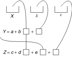
Path models do not infer causation from associa-tion. Instead, path modelsassume causation through response schedules, and – using additional statistical assumptions – estimate causal effects from obser-vational data. The statistical assumptions (indepen-dence, expectation zero, constant variance) justify estimation by ordinary least squares. With large sam-ples, confidence intervals and significance tests would follow. With small samples, the errors would have to follow a normal distribution in order to justifytTests. The box model in Figure 5 illustrates the statistical assumptions. Independent errors with constant dis-tributions are represented as draws made at random with replacement from a box of potential errors [26]. Since the box remains the same from one draw to another, the probability distribution of one draw is the same as the distribution of any other. The distri-bution is constant. Furthermore, the outcome of one draw cannot affect the distribution of another. That is independence. Verifying the causal assumptions (11) and (12), which are about potential outcomes, is a daunting task. The statistical assumptions present dif-ficulties of their own. Assessing the degree to which the modeling assumptions hold is therefore prob-lematic. The difficulties noted earlier – in Yule on poverty, Blau and Duncan on stratification, Gibson on McCarthyism – are systemic.
Embedded in the formalism is the conditional dis-tribution ofY, if we were to intervene and set the value ofX. This conditional distribution is a counter-factual, at least when the study is observational. The conditional distribution answers the question, what would have happened if we had intervened and set X to x, rather than letting Nature take its course?
X
Y = a + b +
Z = c + d + e +
d e
The idea is best suited to experiments or hypothetical experiments.
There are also nonmanipulationist ideas of causa-tion: the moon causes the tides, earthquakes cause property values to go down, time heals all wounds. Time is not manipulable; neither are earthquakes or the moon. Investigators may hope that regression equations are like laws of motion in classical physics. (If position and momentum are given, you can deter-mine the future of the system and discover what would happen with different initial conditions.) Some other formalism may be needed to make this nonma-nipulationist account more precise.
Latent Variables
There is yet another layer of complexity when the variables in the path model remain ‘latent’ – unob-served. It is usually supposed that the manifest vari-ables are related to the latent varivari-ables by a series of regression-like equations (‘measurement models’). There are numerous assumptions about error terms, especially when likelihood techniques are used. In effect, latent variables are reconstructed by some ver-sion of factor analysis and the path model is fitted to the results. The scale of the latent variables is not usu-ally identifiable, so variables are standardized to have mean 0 and variance 1. Some algorithms will infer the path diagram as well as the latents from the data, but there are additional assumptions that come into play. Anderson [7] provides a rigorous discussion of statistical inference for models with latent variables, given the requisite statistical assumptions. He does not address the connection between the models and the phenomena. Kline [46] is a well-known text. Ull-man and Bentler [78] survey recent developments.
A possible conflict in terminology should be men-tioned. In psychometrics and cognate fields, ‘struc-tural equation modeling’ (typically, path modeling with latent variables) is sometimes used for causal inference and sometimes to get parsimonious descrip-tions of covariance matrices. For causal inference, questions of stability are central. If no causal infer-ences are made, stability under intervention is hardly relevant; nor are underlying equations ‘structural’ in the econometric sense described earlier. The statisti-cal assumptions (independence, distributions of error terms constant across subjects, parametric models for error distributions) would remain on the table.
Literature Review
There is by now an extended critical literature on statistical models, starting perhaps with the exchange between Keynes [44, 45] and Tinbergen [77]. Other familiar citations in the economics literature include Liu [52], Lucas [53], and Sims [71]. Manski [54] returns to the under-identification problem that was posed so sharply by Liu and Sims. In brief, a pri-oriexclusion of variables from causal equations can seldom be justified, so there will typically be more parameters than data. Manski suggests methods for bounding quantities that cannot be estimated. Sims’ idea was to use simple, low-dimensional models for policy analysis, instead of complex-high dimensional ones. Leamer [48] discusses the issues created by specification searches, as does Hendry [35]. Heck-man [33] traces the development of econometric thought from Haavelmo and Frisch onwards, stress-ing the role of ‘structural’ or ‘invariant’ parameters, and ‘potential outcomes’. Lucas too was concerned about parameters that changed under intervention. Engle, Hendry, and Richard [17] distinguish sev-eral kinds of exogeneity, with different implications for causal inference. Recently, some econometricians have turned to natural experiments for the evaluation of causal theories. These investigators stress the value of careful data collection and data analysis. Angrist and Krueger [8] have a useful survey.
of Kahneman and Tversky, Sen [69] gives a far-reaching critique of rational choice theory. This theory has its place, but also leads to ‘serious descriptive and predictive problems’.
Almost from the beginning, there were cri-tiques of modeling in other social sciences too [64]. Bernert [10] reviews the historical development of causal ideas in sociology. Recently, modeling issues have been much canvassed in sociology. Abbott [2] finds that variables like income and education are too abstract to have much explanatory power, with a broader examination of causal modeling in Abbott [3]. He finds that ‘an unthinking causalism today pervades our journals’; he recommends more emphasis on descriptive work and on middle-range theories. Berk [9] is skeptical about the possibility of inferring causation by modeling, absent a strong theoretical base. Clogg and Haritou [14] review diffi-culties with regression, noting that you can too easily include endogenous variables as regressors.
Goldthorpe [30, 31, 32] describes several ideas of causation and corresponding methods of statisti-cal proof, with different strengths and weaknesses. Although skeptical of regression, he finds rational choice theory to be promising. He favors use of descriptive statistics to determine social regularities, and statistical models that reflect generative pro-cesses. In his view, the manipulationist account of causation is generally inadequate for the social sci-ences. Hedstr¨om and Swedberg [34] present a lively collection of essays by sociologists who are quite skeptical about regression models; rational choice theory also takes its share of criticism. There is an influential book by Lieberson [50], with a follow-up by Lieberson and Lynn [51]. N´ı Bhrolch´ain [60] has some particularly forceful examples to illustrate the limits of modeling. Sobel [72] reviews the litera-ture on social stratification, concluding that ‘the usual modeling strategies are in need of serious change’. Also see Sobel [73].
Meehl [57] reports the views of an empirical psy-chologist. Also see Meehl [56], with data showing the advantage of using regression to make predictions, rather than experts. Meehl and Waller [58] discuss the choice between two similar path models, viewed as reasonable approximations to some underlying causal structure, but do not reach the critical question – how to assess the adequacy of the approximation. Steiger [75] has a critical review of structural equa-tion models. Larzalere and Kuhn [47] offer a more
general discussion of difficulties with causal infer-ence by purely statistical methods. Abelson [1] has an interesting viewpoint on the use of statistics in psychology.
There is a well-known book on the logic of causal inference, by Cook and Campbell [15]. Also see Shadish, Cook, and Campbell [70], which has among other things a useful discussion of manipulationist versus nonmanipulationist ideas of causation. In polit-ical science, Duncan [16] is far more skeptpolit-ical about modeling than Blau and Duncan [12]. Achen [5, 6] provides a spirited and reasoned defense of the mod-els. Brady and Collier [13] compare regression meth-ods with case studies; invariance is discussed under the rubric of causal homogeneity.
Recently, strong claims have been made for non-linear methods that elicit the model from the data and control for unobserved confounders [63, 74]. How-ever, the track record is not encouraging [22, 24, 25, 39]. Cites from other perspectives include [55, 61, 62], as well as [18, 19, 20, 21, 23].
The statistical model for causation was proposed by Neyman [59]. It has been rediscovered many times since: see, for instance, [36, Section 9.4]. The setup is often called ‘Rubin’s model’, but that simply mis-takes the history. See the comments by Dabrowska and Speed on their translation of Neyman [59], with a response by Rubin; compare to Rubin [68] and Hol-land [37]. HolHol-land [37, 38] explains the setup with a super-population model to account for the random-ness, rather than individualized error terms. Error terms are often described as the overall effects of fac-tors omitted from the equation. But this description introduces difficulties of its own, as shown by Pratt and Schlaifer [65, 66]. Stone [76] presents a super-population model with some observed covariates and some unobserved. Formal extensions to observational studies – in effect, assuming these studies are exper-iments after suitable controls have been introduced – are discussed by Holland and Rubin among others.
Conclusion
developed. Natural variation needs to be identified and exploited. Data must be collected. Confounders need to be considered. Alternative explanations have to be exhaustively tested. Before anything else, the right question needs to be framed. Naturally, there is a desire to substitute intellectual capital for labor. That is why investigators try to base causal inference on statistical models. The technology is relatively easy to use, and promises to open a wide variety of ques-tions to the research effort. However, the appearance of methodological rigor can be deceptive. The models themselves demand critical scrutiny. Mathematical equations are used to adjust for confounding and other sources of bias. These equations may appear formidably precise, but they typically derive from many somewhat arbitrary choices. Which variables to enter in the regression? What functional form to use? What assumptions to make about parameters and error terms? These choices are seldom dictated either by data or prior scientific knowledge. That is why judgment is so critical, the opportunity for error so large, and the number of successful applications so limited.
Author’s footnote
Richard Berk, Persi Diaconis, Michael Finkelstein, Paul Humphreys, Roger Purves, and Philip Stark made useful comments. This paper draws on man [19, 20, 22 – 24]. Figure 1 appeared in Freed-man [21, 24]; figure 2 is redrawn from Blau and Duncan [12]; figure 3, from Gibson [28], also see Freedman [20].
References
[1] Abelson, R. (1995).Statistics as Principled Argument,
Lawrence Erlbaum Associates, Hillsdale.
[2] Abbott, A. (1997). Of time and space: the contemporary
relevance of the Chicago school, Social Forces 75,
1149–1182.
[3] Abbott, A. (1998). The Causal Devolution,Sociological
Methods and Research27, 148–181.
[4] Achen, C. (1977). Measuring representation: perils of
the correlation coefficient,American Journal of Political
Science21, 805–815.
[5] Achen, C. (1982). Interpreting and Using Regression,
Sage Publications.
[6] Achen, C. (1986). The Statistical Analysis of
Quasi-Experiments, University of California Press, Berkeley.
[7] Anderson, T.W. (1984). Estimating linear statistical
relationships,Annals of Statistics12, 1–45.
[8] Angrist, J.D. & Krueger, A.K. (2001). Instrumental
variables and the search for identification: from supply
and demand to natural experiments,Journal of Business
and Economic Statistics19, 2–16.
[9] Berk, R.A. (2003).Regression Analysis: A Constructive
Critique, Sage Publications, Newbury Park.
[10] Bernert, C. (1983). The career of causal analysis in
American sociology, British Journal of Sociology 34,
230–254.
[11] Blalock, H.M. (1989). The real and unrealized
contribu-tions of quantitative sociology, American Sociological
Review54, 447–460.
[12] Blau, P.M. & Duncan O.D. (1967). The American
Occupational Structure, Wiley. Reissued by the Free Press, 1978. Data collection described on page 13, coding of education on pages 165–66, coding of status on pages 115–27, correlations and path diagram on pages 169–170.
[13] Brady, H. & Collier, D., eds (2004).Rethinking Social
Inquiry: Diverse Tools, Shared Standards, Rowman & Littlefield Publishers.
[14] Clogg, C.C. & Haritou, A. (1997). The regression
method of causal inference and a dilemma confronting
this method, in Causality in Crisis, V. McKim &
S. Turner, eds, University of Notre Dame Press, pp. 83–112.
[15] Cook, T.D. & Campbell, D.T. (1979).
Quasi-Experi-mentation: Design & Analysis Issues for Field Settings, Houghton Mifflin, Boston.
[16] Duncan, O.D. (1984). Notes on Social Measurement,
Russell Sage, New York.
[17] Engle, R.F., Hendry, D.F. & Richard, J.F. (1983).
Exogeneity,Econometrica51, 277–304.
[18] Freedman, D.A. (1985). Statistics and the scientific
method, inCohort Analysis in Social Research: Beyond
the Identification Problem, W.M. Mason & S.E. Fien-berg, eds, Springer-Verlag, New York, pp. 343–390, (with discussion).
[19] Freedman, D.A. (1987). As others see US: a case study
in path analysis, Journal of Educational Statistics 12,
101–223, (with discussion), Reprinted in The Role of
Models in Nonexperimental Social Science, J. Shaffer, ed., AERA/ASA, Washington, 1992, pp. 3–125.
[20] Freedman, D.A. (1991). Statistical models and shoe
leather, in Sociological Methodology 1991, Chap. 10,
Peter Marsden, ed., American Sociological Association, Washington, (with discussion).
[21] Freedman, D.A. (1995). Some issues in the foundation
of statistics, Foundations of Science 1, 19–83, (with
discussion), Reprinted inSome Issues in the Foundation
of Statistics, B.C. van Fraassen, ed., (1997). Kluwer, Dordrecht, pp. 19–83 (with discussion).
[22] Freedman, D.A. (1997). From association to causation
via regression, in Causality in Crisis? V. McKim &
Bend, pp. 113–182, with discussion. Reprinted in
Advances in Applied Mathematics18, 59–110.
[23] Freedman, D.A. (1999). From association to
causa-tion: some remarks on the history of statistics,
Sta-tistical Science14, 243–258, Reprinted inJournal de la Soci´et´e Fran¸caise de Statistique 140, (1999). 5–32,
and inStochastic Musings: Perspectives from the
Pio-neers of the Late 20th Century, J. Panaretos, ed., (2003). Lawrence Erlbaum, pp. 45–71.
[24] Freedman, D.A. (2004). On specifying graphical models
for causation, and the identification problem,Evaluation
Review26, 267–293.
[25] Freedman, D.A. & Humphreys, P. (1999). Are there
algorithms that discover causal structure?Synthese121,
29–54.
[26] Freedman, D.A., Pisani, R. & Purves, R.A. (1998).
Statistics, 3rd Edition, W. W. Norton, New York.
[27] Gauss, C.F. (1809). Theoria Motus Corporum
Coele-stium, Perthes et Besser, Hamburg, Reprinted in 1963 by Dover, New York.
[28] Gibson, J.L. (1988). Political intolerance and political
repression during the McCarthy red scare, APSR 82,
511–529.
[29] Gigerenzer, G. (1996). On narrow norms and vague
heuristics,Psychological Review103, 592–596.
[30] Goldthorpe, J.H. (1998).Causation, Statistics and
Soci-ology, Twenty-ninth Geary Lecture, Nuffield College, Oxford. Published by the Economic and Social Research Institute, Dublin.
[31] Goldthorpe, J.H. (2000).On Sociology: Numbers,
Nar-ratives, and Integration of Research and Theory, Oxford University Press.
[32] Goldthorpe, J.H. (2001). Causation, Statistics, and
Soci-ology,European Sociological Review17, 1–20.
[33] Heckman, J.J. (2000). Causal parameters and policy
analysis in economics: a twentieth century retrospective,
The Quarterly Journal of EconomicsCVX, 45–97.
[34] Hedstr¨om, P. & Swedberg, R., eds (1998).Social
Mech-anisms, Cambridge University Press.
[35] Hendry, D.F. (1993). Econometrics–Alchemy or
Sci-ence?Blackwell, Oxford.
[36] Hodges, J.L. Jr. and Lehmann, E. (1964).Basic Concepts
of Probability and Statistics, Holden-Day, San Francisco.
[37] Holland, P. (1986). Statistics and causal inference,
Jour-nal of the American Statistical Association8, 945–960.
[38] Holland, P. (1988). Causal inference, path analysis, and
recursive structural equation models, in Sociological
Methodology 1988, Chap. 13, C. Clogg, ed., American Sociological Association, Washington.
[39] Humphreys, P. & Freedman, D.A. (1996). The grand
leap,British Journal for the Philosophy of Science 47,
113–123.
[40] Kahneman, D., Slovic, P., and Tversky, A., eds (1982).
Judgment under Uncertainty: Heuristics and Biases, Cambridge University Press.
[41] Kahneman, D. & Tversky, A. (1974). Judgment
under uncertainty: heuristics and bias, Science 185,
1124–1131.
[42] Kahneman, D. & Tversky, A. (1996). On the reality of
cognitive illusions,Psychological Review103, 582–591.
[43] Kahneman, D. & Tversky, A., eds (2000). Choices,
Values, and Frames, Cambridge University Press.
[44] Keynes, J.M. (1939). Professor Tinbergen’s method,The
Economic Journal49, 558–570.
[45] Keynes, J.M. (1940). Comment on Tinbergen’s response,
The Economic Journal50, 154–156.
[46] Kline, R.B. (1998).Principles and Practice of Structural
Equation Modeling, Guilford Press, New York.
[47] Larzalere, R.E. & Kuhn, B.R. (2004). The intervention
selection bias: an underrecognized confound in
interven-tion research,Psychological Bulletin130, 289–303.
[48] Leamer, E. (1978).Specification Searches, John Wiley,
New York.
[49] Legendre, A.M. (1805). Nouvelles m´ethodes pour la
d´etermination des orbites des com`etes, Courcier, Paris. Reprinted in 1959 by Dover, New York.
[50] Lieberson, S. (1985). Making it Count, University of
California Press, Berkeley.
[51] Lieberson, S. & Lynn, F.B. (2002). Barking up the wrong
branch: alternative to the current model of sociological
science,Annual Review of Sociology28, 1–19.
[52] Liu, T.C. (1960). Under-identification, structural
estima-tion, and forecasting,Econometrica28, 855–865.
[53] Lucas, R.E. Jr. (1976). Econometric policy evaluation: a
critique, in K. Brunner & A. Meltzer, eds,The Phillips
Curve and Labor Markets, Vol. 1 of the Carnegie-Rochester Conferences on Public Policy, supplementary series to the Journal of Monetary Economics, North-Holland, Amsterdam, pp. 19–64. (With discussion.)
[54] Manski, C.F. (1995). Identification Problems in the
Social Sciences, Harvard University Press.
[55] McKim, V. & Turner, S., eds (1997). Causality in
Crisis? Proceedings of the Notre Dame Conference on Causality, University of Notre Dame Press.
[56] Meehl, P.E. (1954). Clinical Versus Statistical
Predic-tion: A Theoretical Analysis and a Review of the Evi-dence, University of Minnesota Press, Minneapolis.
[57] Meehl, P.E. (1978). Theoretical risks and tabular
aster-isks: Sir Karl, Sir Ronald, and the slow progress of soft
psychology,Journal of Consulting and Clinical
Psychol-ogy46, 806–834.
[58] Meehl, P.E. & Waller, N.G. (2002). The path
analy-sis controversy: a new statistical approach to strong
appraisal of verisimilitude, Psychological Methods 7,
283–337. (with discussion).
[59] Neyman, J. (1923). Sur les applications de la th´eorie
des probabilit´es aux experiences agricoles: Essai des
principes, Roczniki Nauk Rolniczki10, 1–51,in Polish.
English translation by Dabrowska, D. & Speed, T.
(1990).Statistical Science5, 463–480, with discussion.
[60] N´ı Bhrolch´ain, M. (2001). Divorce effects and causality
in the social sciences,European Sociological Review17,
33–57.
[61] Oakes, M.W. (1986).Statistical Inference, Epidemiology
[62] Pearl, J. (1995). Causal diagrams for empirical research,
Biometrika82, 669–710, with discussion.
[63] Pearl, J. (2000). Causality: Models, Reasoning, and
Inference, Cambridge University Press.
[64] Platt, J. (1996). A History of Sociological Research
Methods in America, Cambridge University Press.
[65] Pratt, J. & Schlaifer, R. (1984). On the nature and
dis-covery of structure,Journal of the American Statistical
Association79, 9–21.
[66] Pratt, J. & Schlaifer, R. (1988). On the interpretation
and observation of laws, Journal of Econometrics39,
23–52.
[67] Quetelet, A. (1835).Sur l’homme et le d´eveloppement
de ses facult´es, Ou essai de physique sociale, Bachelier, Paris.
[68] Rubin, D. (1974). Estimating causal effects of treatments
in randomized and nonrandomized studies, Journal of
Educational Psychology66, 688–701.
[69] Sen, A.K. (2002). Rationality and Freedom, Harvard
University Press.
[70] Shadish, W.R., Cook, T.D. & Campbell, D.T. (2002).
Experimental and Quasi-Experimental Designs for Gen-eralized Causal Inference, Houghton Mifflin, Boston.
[71] Sims, C.A. (1980). Macroeconomics and reality,
Econo-metrica48, 1–47.
[72] Sobel, M.E. (1998). Causal inference in statistical
mod-els of the process of socioeconomic achievement–a case
study,Sociological Methods & Research27, 318–348.
[73] Sobel, M.E. (2000). Causal inference in the social
sciences,Journal of the American Statistical Association
95, 647–651.
[74] Spirtes, P., Glymour, C., and Scheines, R. (1993).
Causation, Prediction, and Search, 2nd Edition 2000,
Springer Lecture Notes in Statistics, Vol. 81, Springer-Verlag, MIT Press, New York.
[75] Steiger, J.H. (2001). Driving fast in reverse,Journal of
the American Statistical Association96, 331–338.
[76] Stone, R. (1993). The assumptions on which causal
inferences rest,Journal of the Royal Statistical Society
Series B55, 455–466.
[77] Tinbergen, J. (1940). Reply to Keynes, The Economic
Journal50, 141–154.
[78] Ullman, J.B. and Bentler, P.M. (2003). Structural
equation modeling, in I.B. Weiner, J.A. Schinka &
W.F. Velicer, eds, Handbook of Psychology. Volume
2: Research Methods in Psychology, Wiley, Hoboken, pp. 607–634.
[79] Yule, G.U. (1899). An investigation into the causes of
changes in Pauperism in England, chiefly during the last
two intercensal decades,Journal of the Royal Statistical
Society62, 249–295.