UAV-BASED POINT CLOUD GENERATION FOR OPEN-PIT MINE MODELLING
M. Shahbazi a, *, G. Sohn b, J. Théau a, P. Ménard c
a
Dept. of Applied Geomatics, Université de Sherbrooke, Boul. de l'Université, Sherbrooke, Québec, Canada- (mozhdeh.shahbazi, jerome.theau)@usherbrooke.ca
b
Dept. of Geomatics Engineering, York University, Keele Street, Toronto, Ontario, Canada- [email protected] c
Centre de géomatique du Québec, Saguenay, Québec, Canada- [email protected]
KEY WORDS: Unmanned Aerial Vehicle, System Integration, Sensor Calibration, Structure from Motion, Sparse and Dense Matching, Open-Pit Mine, Three-dimensional Modelling
ABSTRACT:
Along with the advancement of unmanned aerial vehicles (UAVs), improvement of high-resolution cameras and development of vision-based mapping techniques, unmanned aerial imagery has become a matter of remarkable interest among researchers and industries. These images have the potential to provide data with unprecedented spatial and temporal resolution for three-dimensional (3D) modelling. In this paper, we present our theoretical and technical experiments regarding the development, implementation and evaluation of a UAV-based photogrammetric system for precise 3D modelling. This system was preliminarily evaluated for the application of gravel-pit surveying. The hardware of the system includes an electric powered helicopter, a 16-megapixels visible camera and inertial navigation system. The software of the system consists of the in-house programs built for sensor calibration, platform calibration, system integration and flight planning. It also includes the algorithms developed for structure from motion (SfM) computation including sparse matching, motion estimation, bundle adjustment and dense matching.
* Corresponding author
1. INTRODUCTION 1.1 UAV-based 3D Modelling
Recently, low-altitude imagery has become a matter of remarkable interest among researchers in both photogrammetry and computer-vision communities. The 3D models generated from UAV imagery can serve various applications ranging from natural resource management to civil engineering (Shahbazi et al., 2014; Liu et al., 2014). In spite of the advantages introduced by UAVs and despite the commercial and open-source efforts, unmanned mapping systems are still requiring investigations and considerations in terms of efficient data processing. There are basic differences between the features of unmanned aerial systems and those of traditional aerial systems, which cause challenging issues in the procedure of SfM computation and 3D modelling. These features are briefly discussed in this section.
Small-format cameras cover only a small area per image. Therefore, in most of the applications, mosaicking is required. In order to provide geospatially valid mosaics, accurate geo-referencing is mandatory too. To this end, two different methods might be applied; first direct geo-referencing via navigation sensors, second indirect exterior orientation (EO) estimation via image observations and subsequent geo-referencing via ground control points (GCPs). The accuracy of direct geo-referencing is mainly influenced by the accuracy of the navigation sensors and the platform calibration (Turner et al., 2014). On the other hand, the accuracy of indirect geo-referencing is affected by the positioning accuracy of GCPs and the accuracy of tie-point detection among overlapping images, namely sparse matching (Turner et al., 2012).
Despite the advantages of consumer-grade cameras in terms of price, weight and resolution, yet, their unstable lens and sensor mounts put noticeable concern in precise 3D modelling.
Therefore, internal camera calibration must be performed. When requiring metric accuracies, offline calibration of the camera is suggested (Remondino and Fraser, 2006). However, on-the-mission vibrations can affect the calibration parameters of the camera to some extent (Rieke-Zapp et al., 2009). Therefore, the offline calibration performed in laboratory may no longer be valid on the flight campaign. A solution to this problem is to calibrate the camera by adding the systematic error terms to the block bundle adjustment (BBA), namely self-calibration.
The solutions and software packages, which are developed for different stages of SfM computation, must deal with specific features of unmanned aerial images. The most distinctive characteristics of UAV images are: i) large perspective distortion and scale changes due to oblique photography and low flight altitude in comparison with terrain relief, ii) high matching error due to uneven distribution of feature points, motion blur, occlusion or foreground motion of the features and noticeable radiometric changes (Zhang et al., 2011; Haala et al., 2013). Several studies have been performed in recent years to assess the performance of UAVs in 3D modelling applications. Valuable reviews of such studies can be found in Colomina and Molina (2014) and Nex and Remondino (2014).
1.2 Open-Pit Mine Modelling
Since the main application of the system studied in this paper is gravel-pit surveying, the main problematic which justifies the necessity of developing new mapping technologies for gravel pits is discussed in this section. In general, gravel mining impacts the surrounding environment in many ways, and those impacts must be monitored frequently. Ground subsidence, landslide and slope instability are the most dangerous issues at gravel pits, especially considering the lubricious nature of gravel (Herrera et al., 2010). Previous studies on geotechnical The International Archives of the Photogrammetry, Remote Sensing and Spatial Information Sciences, Volume XL-1/W4, 2015
risk assessment have shown that the topographic data must provide a ground resolution of one to three centimetres in order to predict such events (Ivory, 2012; Francioni et al., 2014).
Furthermore, mine managers have to report the amount of extracted mass, left over tailing dumps and waste materials on a regular basis according to governmental regulations. Therefore, volumetric change measurement within a gravel pit is mandatory. The map-scale required for volumetric measurement in earthworks is usually between 1:4,000 and 1:10,000 (Patikova, 2004). Given an imaging sensor with 10 μm pixels, the ground resolution must be between 4 to 10 centimetres per pixel to provide such a scale range.
Regarding the above-mentioned arguments, mapping and monitoring of a gravel pit requires high-quality topographic and visual data. Considering the required spatial and temporal resolution, coverage area, speed of measurement, and safety criteria, UAVs can be better solutions for gravel-pit mapping in comparison with manned aerial systems or land surveying techniques. Therefore, open-pit mine mapping is slowly becoming a practical application of UAVs (McLeod et al., 2013; Hugenholtz et al., 2014).
1.3 Article Structure and Contributions
Considering the arguments given above, the structure of this paper is divided into two principal parts: data acquisition and data processing. In the first part of the paper, we are aiming to discuss and address the main issues regarding the equipment, sensor calibration, platform calibration and system integration. Several aspects of these tasks are discussed in Section 2, and the intermediate experimental results for each particular task are presented as well. Then, our experiments for fieldwork planning and data acquisition as well as their results are presented in Section 3.
In the second part of the paper, we present our algorithms for SfM computation (Section 4) and their corresponding results (Section 5). These algorithms bring up the following contributions. Firstly, a new method, mainly based on genetic algorithm, is proposed for robust sparse matching and motion estimation. It provides several advantages in comparison with the existing algorithms in the state-of-the-art including the improved computational efficiency and robustness against degeneracy, poor camera motion models and noise. Secondly, several BBA strategies are assessed, and a new strategy is proposed in order to control the effects of on-the-job, self-calibration on the accuracy of other outputs. Finally, a dense matching algorithm based on the intrinsic-curves theory is proposed, which is a matching strategy independent of the spatial space. The advantage of this algorithm is that the computational efficiency of matching would not change, regardless of the irregularity of the disparity map. Besides, the application of intrinsic curves causes the matching to be robust against occlusions.
2. UNMANNED AERIAL SYSTEM DEVELOPMENT 2.1 Platform, Sensors and Processor
The platform used in this project is a helicopter, called Responder, which is built by ING Robotic Aviation1
. This platform is powered by electricity with operational endurance
1
www.ingrobotic.com
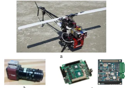
of approximately 40 minutes. It provides up to 12 kilograms payload capacity, which is more than adequate for our sensors and processor weighing less than 3.5 kilograms. Figure 1 presents the platform and its on-board elements.
Two digital cameras were tested in this study, Prosilica GE4900C visible camera and Prosilica GT1920C high-frame-rate camera. While both cameras provide high-resolution data, the GT1920C has the advantage of providing 40 frames per second at full resolution. However, the main disadvantage of this camera is the small-size sensor, which makes the 3D modelling process more difficult. Since better results in terms of accuracy and efficiency have been obtained via GE4900C, only this camera will be further discussed. This camera has an approximate sensor size of 36x24 mm, and a 35 mm, F-adjustable lens was set with it.
The navigation sensor used in this project is an industrial-grade, GPS-aided inertial navigation system (INS), MIDGII from Microbotics Inc2
. Theoretically, the unit measures pitch and roll with 0.4 degree and heading (yaw) with 1-2 degrees of accuracy. The position accuracy is approximately 2-5 meters.
The computer used in this project is an ultra-small, single-board system, which is based on 1.7GHz Intel Core™ i7 processor. SATA III ports for on-the-flight, external storage purposes, Gigabit Ethernet ports for connecting the camera, USB port for connecting the INS and wireless adaptor for remote control are among the required features of the board. We stacked the board together with a 108 Watt power supply, which receives electricity from the battery pack and distributes regulated DC voltage to the processing unit and other sensors. With this configuration, the embedded system is capable of acquiring, logging, and storing data during almost 70 minutes.
a
b c Figure 1. The aerial system, a) platform, b) sensors, c) computer
2.2 System Integration
The control subsystem in the UAV photogrammetric system is responsible for several tasks, including power control, controlling the data acquisition parameters, data logging, data storage, and time synchronization. The brief integration scheme developed in this project is illustrated in Figure 2. To create these controllers, an object-oriented, cross-platform C++ program is developed. The software solution contains three main classes: INS, Camera, and Clock. The Clock controller is responsible to record the accurate time of all the events (camera exposure-end and INS message reception) via the system-wide, real-time clock. The functions of INS class are responsible for
2
www.microboticsinc.com
communicating with the INS, receiving the high-frequency data, parse them and log them. The GPS-time of INS messages is also assigned to a static variable communicating with the Camera class. The Camera class is responsible for communicating with the camera, setting acquisition parameters, logging images and geo-tagging each image with the INS message received at the exposure-end-event epoch of that images. This synchronization is performed via multithreading and mutual communication between classes. Our experiments showed that the GPS time tagged to any image via the INS is only 117 milliseconds delayed from the exact time of the exposure-end event.
Figure 2. Integration scheme of the system and its components
2.3 Camera Calibration
In applications where metric accuracies are required, offline camera calibration is suggested (Remondino and Fraser, 2006). The network geometry and precise target detection are very important factors that affect the camera parameters. Therefore, off-line calibration can achieve higher accuracy and precision in comparison with on-the-job calibration. The practical steps of off-line camera calibration developed in this study include:
i) deciding the parameters of the calibration model: In addition to the internal orientation (IO) parameters (the offsets of the camera principal point and the focal length), the Brown's additional parameters for digital cameras are applied to model the systematic errors (Brown, 1971). The error sources considered in this model include radial and tangential lens distortions and sensor, in-plane distortions.
ii) designing and establishing a test-field with signalized targets: Two factors, size and depth, must be considered when designing the test-field. Size and shape of the targets are also other important elements which must be carefully considered in order to facilitate very accurate target positioning. The 3D coordinates of the targets are accurately measured using a spatial station for assessment purposes. The test-field is shown in Figure 4(a).
iii) setting up the camera at different orientations, and photographing the test-field: Having various orientations and depths are necessary to provide a stable network geometry. This way, it can be ensured that the calibration parameters are not affected by/dependant to the network geometry (Fraser, 1997). iv) detecting and positioning the targets on the images: The targets are designed as black and white rings. Thus, once the image of the circular target is deformed under any linear transformation, it appears as an ellipse. Therefore, a technique of ellipse detection based on edge-detection and ellipse fitting is developed to position and label the targets very accurately. v) performing free-network calibration to calculate the parameters and correcting images to restore undistorted images.
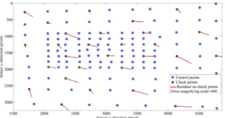
The off-line calibration was repeated several times before and after various missions. The accuracy of average parameters was
assessed using check data. To this end, several images were captured from the test-fields. Controlled resection using camera calibration parameters was performed, and EO parameters of the images were determined. For some checkpoints (targets not assisted in resection), the 3D ground-coordinates of the targets were back-projected to the images, and the residuals from their actual positions were measured (Figure 3). The mean and standard deviation (StD) of the residuals on the checkpoints at x- and y-directions were 0.320.18 and 0.200.16 pixels, respectively. The residuals showed how efficiently the calibration parameters affected the accuracy of EO.
Figure 3. Residuals on checkpoints after camera calibration
2.4 Platform Calibration
The navigation and imaging data are measured at different coordinate systems. With this regard, the main goal of platform calibration is to, first, measure the offset vector between the perspective center of the camera and the center of the INS body-fixed system (lever-arm); second, to determine the rotations of the imaging system axes with respect to the INS system (bore-sight angles). Since the INS used in this study is utilizing consumer-grade GPS, the positioning accuracy of few meters eliminates the need for level-arm calibration.
Normally, platform calibration is essential when direct geo-referencing of images is considered. However, in this project, we are not interested in direct geo-referencing of images, as we are looking for higher accuracy levels. Nevertheless, we are still looking for the direct EO to be capable of approximately positioning the GCPs on images. Then, the rough position of GCPs can be refined using image processing techniques. For facilitating the platform calibration, we stacked the camera and the INS together, in a fixed status (Figure 1(b)). Consequently, we could calibrate the platform before installing the sensors on the UAV. A test-field with circular targets was established (Figure 4(b)), and the targets were accurately measured via the spatial station. The spatial station, itself, has been stationed using precisely positioned points on the ground. Then, images were acquired from the test-field while logging the INS data. The EO parameters of the images were calculated via controlled space resection, and their comparison with the navigation data of INS resulted in the platform calibration parameters.
a b The International Archives of the Photogrammetry, Remote Sensing and Spatial Information Sciences, Volume XL-1/W4, 2015
Figure 4. The test-fields for a) camera calibration, b) platform calibration
3. DATA ACQUISITION EXPERIMENTS 3.1 Planning
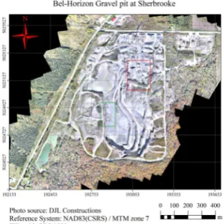
The data for this study was acquired from a gravel pit, located at Sherbrooke, QC, Canada. The extent of the mine is shown in Figure 5. Two main zones, which were considered for our tests are shown by red and green rectangles in Figure 5. The red zone represents a part of the gravel pit, which is covered by piles of gravel, and the green zone represents the cliffs, where the rock is dynamited for extraction.
Figure 5. Study area, the open-pit mine located at Sherbrooke
Planning the fieldwork is an important part of the project. The quality of the control and check data as well as the images depends highly on this stage. In order to plan the flight itself, there are several free software packages (e.g. Mission Planner). However, a simple program is developed in this study to satisfy our specific needs for both flight and surveying planning. The software is able to decide the flight characteristics based on the terrain relief, time of flight, drone characteristics, required resolution and overlap, as well as camera features. Besides, it determines the optimal number and distribution of required ground control points, and determines the optimal size for designing the targets to indicate GCPs. GCPs were signalized using circular targets with binary crosshairs at the centre (Figure 6(b)). We used sharp colors, red and yellow, for the background to make them be distinguishable from the natural objects in the scene. They were also labelled with easily recognizable labels, both in terms of size and shape.
3.2 Fieldwork
The first essential task to start the fieldwork was to initialize the GPS base receiver, whose coordinates were required to perform real time kinematic positioning. We recorded the base station observations for more than 10 hours, and processed them via CSRS-PPP service provided by Natural Resources Canada3. The position of the base point was determined with 2-5 millimeters horizontal and 12 millimeters vertical absolute accuracy. Afterwards, the next task was to install the targets and measure their positions using RTK GPS system. Once the image acquisition was terminated, the terrestrial surveying for gathering check data was performed. In order to collect the
3
http://webapp.geod.nrcan.gc.ca/geod/tools-outils
check data, a Trimble VX Spatial Station was used. The station was setup over ground marks whose coordinates were measured with the RTK system, and laser scanning was conducted. Figure 6(a) presents an example of the way the GCPs and scanner stations were configured for the cliffs zone.
a
b
Figure 6. Fieldwork elements, a) Configuration of GCPs and VX scanner stations for the cliffs zone, b) signalized target patterns for GCPs
3.3 Preliminary Results
In order to quickly check the quality of acquired data, the images and their geo-logs were processed by the commercial photogrammetric software, Pix4D4. The 3D point clouds and the aerial mosaics were generated via this software. Afterwards, the CloudCompare5 open-source software was applied to compare the aerial point clouds with the terrestrial laser point clouds. In some cases, image enhancement by pre-processing was also applied to improve the results. For instance, to remove the effect of shadows at cliffs zone, a shadow-detection and removal algorithm based on luminance processing was used.
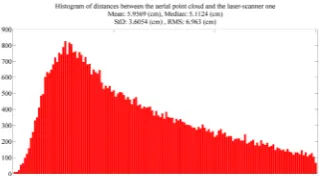
Figure 7 visualizes the aerial mosaic (with average ground resolution of 1.3 cm) and 3D point cloud from the cliff zone. Figure 8 represents the comparison between the laser point cloud and the image-based one, in terms of the distance between two clouds. The average horizontal distance between the aerial and the laser point clouds was 3.29 cm, and the average vertical distance between them was 2.04 cm.
a
b
Figure 7. Visualization of the preliminary 3D products from the developed unmanned aerial system, a) mosaic, b) point cloud
4
www.pix4d.com 5
www.cloudcompare.org
Figure 8. The accuracy analysis of the point cloud, histogram of 3D distances between image and laser point clouds in cm.
4. STRUCTURE FROM MOTION COMPUTATION 4.1 Sparse Matching and Motion Estimation
The sparse matching and robust motion estimation technique used in this study is mainly based on genetic algorithms (GA). It can be considered as an alternative to RANSAC-like techniques where the random search is replaced with evolutionary search. The algorithm benefits from other novel features such as: i) sampling based spatial distribution of points which is effective both against degeneracy and ill-configuration, ii) fast linear calculation of epipolar geometry without encountering exceptions in cases of poor motion models, iii) adaptive thresholding to detect the inlier correspondences, which makes the algorithm robust against noise and outliers.
Basically, GA intends to find a subset of inliers from which the near-optimal motion model (fundamental matrices) can be estimated. To this end, it encodes the putative correspondences from feature-based matching into a cellular environment. Then, several minimal sets of the correspondences are sampled. A guided-sampling strategy based on the spatial distribution of the points is used to this end. The whole set of minimal sample sets forms the population. In any iteration of the evolution, the parent individuals in the population are evaluated against an objective function. The objective function is based on the concept of least trimmed squares. Then, the genetic operators are performed on the selected parents; i.e. they keep being crossed-over, mutated and/or randomized to produce a new population. These iterations go on the same way until reaching an optimal solution, which cannot be improved anymore by younger populations. At the end, an adaptive thresholding scheme is applied to detect all the inlier correspondences based on the estimated motion models. The details of this algorithm can be found in our recent publication (Shahbazi et al., 2015).
An important step before sparse matching is to decide which image pairs should be matched. In other words, image connectivity model should be determined. To this end, the method proposed by Ai et al. (2015) is applied. The ground fields of view (FoV) of cameras are calculated based on their direct EO parameters. Then, stereo pairs with an overlap area greater than a threshold are considered to have connection.
4.2 GCP Detection and Block Bundle Adjustment
Once the motion parameters (relative orientation) are estimated, the direct EO parameters can be refined. It is always beneficial to make sure that one reference image in the dataset contains three or more GCPs. Therefore, the EO of that image can be determined accurately and the EO of other images can be updated using both the motion parameters relative to the reference one and their direct EO parameters. The EO data and
the coordinates of GCPs are then used to locate GCPs on images. The error margin of the approximate EO parameters is also applied to find the uncertainty of the GCPs locations on the images, by defining their covariance error ellipses. Simple colour-based edge detection is used to find the red/yellow edges inside the error ellipse and locate the candidate GCPs more accurately. Afterwards, a similar ellipse detection method as explained in section 2.3 is used to find the exact position of the GCPs on the images. Although this process is automatic, the user supervision is still required to check the results manually.
Afterwards, it is time to perform block bundle adjustment (BBA). The aim of bundle adjustment is to simultaneously determine the 3D coordinates of tie points, the EO parameters and camera calibration parameters according to the co-linearity observation equations. Since, the absolute accuracy of GCPs is determined in the surveying process, therefore, it is essential to apply them in the BBA. To this end, different BBA strategies are tested: i) the minim-constraint least squares optimization (LSO) using the GCPs coordinates as weighted observations, ii) the inner-constraint LSO giving higher weight to GCPs image observations and application of a 7-parameter Helmert transformation to the final results afterward.
As the first conclusion obtained, the first strategy (minim-constraint) is more accurate, since the GCP coordinates can be adjusted as well. The second conclusion is that the camera calibration parameters, calculated either ways, become so sensitive to the number of tie points and stereo pairs. For example, in a test where a hundred of stereo pairs are participating in the BBA, the focal length is calculated to 36.028 mm. However, the same parameter is calculated to 35.102 mm when only twelve high-overlapping images are used. We observed the same sort of results in self-calibration from Pix4D software. Considering error theories, it is obvious that the accuracy of image observations and network configuration can influence the values of calibration parameters. However, they are still physical quantities and are not supposed to change greatly within one specific dataset. Therefore, a modified BBA strategy is proposed in this study.
Since we have performed the offline camera calibration several times, the parameters obtained by these calibration procedures are averaged and their StDs are calculated. A null hypothesis that the measured mean and StD values from these sample parameters can represent the population's real mean and variance at confidence level of 95% is performed with Student's t-test. The results show that this null hypothesis can be supported by the measured data. Therefore, we modify the BBA strategy by considering the camera IO parameters as unknowns with known weight. In other words, they are treated as pseudo-measurements with known variance. As a result, the IO parameters from this pseudo-self-calibration do not change haphazardly as long as a stable network of images is provided.
4.3 Dense Matching and Scene Reconstruction
The goal of dense matching is to determine all/most of the corresponding points visible in a stereo pair, and to determine the disparity map, from which a depth map can be reconstructed. Dense matching is generally performed on rectified images in order to facilitate the matching by restricting it to one direction only (x-axis). There are various techniques in the state-of-the-art for dense matching. Valuable reviews of these techniques can be found in studies performed by Scharstein and Szeliski (2002) and Seitz et al. (2006). Recently, The International Archives of the Photogrammetry, Remote Sensing and Spatial Information Sciences, Volume XL-1/W4, 2015
global and semi-global matching techniques have been popular. In the global techniques, the disparity values are determined by globally minimizing an energy function of disparity. In order to make such an optimization possible, mostly hierarchical/ iterative algorithms are required to limit the search. This increases the computational expenses of matching. Some techniques apply shape priors to reduce the computational expenses of matching specifically in low-textured images. It means that the matching is performed on seed features and the results are extended to the patches/ segments. Mostly, a technique of occlusion detection or visibility handling should also be applied along-with or after the dense matching to avoid or remove the outliers caused by occlusion.
In this study, we take the concept of intrinsic curves proposed by Manduchi (1998) to develop a new dense matching approach. The main improvement that is expected from this technique is the computational efficiency from two aspects: i) performing global matching by eliminating the need to restrict the search area or having initial approximations of disparity range, ii) avoiding occlusions by finding and eliminating invisible matches even before the matching starts.
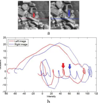
An intrinsic curve is a multi-dimensional representation of a signal, to which different operators are applied. For imges, this definition is clarified with an example. Suppose that the scan-line (a row) in left rectified image of Figure 9 is denoted as l(xl), where xl is the position of each pixel in the left scan-line and l
represents the intensity. Therefore, an intrinsic curve can be constructed as l ( )
C l l , where l is the intensity gradient. Likewise, the intrinsic curve can be constructed for the right scan-line as r ( )
C r r , where r(xr) and (r x r)are the intensity and gradient vectors of the right scan-line. These curves translate the scan-lines from the spatial space to the intensity space. As proved by Manduchi (1998), intrinsic curves are invariant to affine mapping. Therefore, if the transformation between the left and right scan-lines was only an affine geometric one, then the two intrinsic curves would coincide at matching points. However, the images are usually corrupted by noise, non-affine geometric transformations and photometric transformations. Therefore, there is a non-constant variation between the two curves.
a
b
Figure 9. Representation of intrinsic curves, a) left and right rectified images, b) intrinsic curves in the space of intensity
Assumption: Assume a pixel at location l i
x on the left scan-line whose corresponding point on the right scan-line is located at
r i
x . Therefore, the disparity value of this point is l r
i i i
d x x . If the intensities are filtered with a low-pass zero-mean filter, then it can be assumed that the photometric transformation between two scan-lines at the local neighbourhood of these two matches consists of drift (ai) and gain (bi) parameters. Therefore, it can be proved, as follows, that the two points
r l
i i
x x can be corresponding only if the tangents to the right and left curves at these points are equal. In practice, equality should be replaced with a small threshold to take the remaining noise and non-smoothness exceptions into account.
Proof: The right intrinsic curve of point r i
x ( r ( )
i i
C r r ) can be
predicted from the left intrinsic curve ( l ( )
i i
The tangent at this point on left curve ( tan l i
Thus, the tangent at the predicted corresponding point on the right curve ( tan r
Using this assumption, a search for potential matches (hypotheses) is performed along the intrinsic curves of each scan-line. The advantage of this search is that it is performed in the limited space of intensity, and it is independent of the spatial space. This eliminates the need for having an initial range of disparity values. It can be noted that in this search, occluded points have almost no chance to be hypothesized. An example of occlusion occurred in Figure 9 is shown by arrows. It can be seen that the occluded area produces a curve segment in left curve which is not compatible with other segments of the right one. Figure 10 represents the dense point cloud reconstructed from two images, once with the proposed method, and once using the SURE software-solution for multi-view stereo (Rothermel et al., 2012). It can be seen that the proposed algorithm avoids visibility occlusions in the matching process.
Afterward, the matching cost (photo-consistency measure) is measured for the hypothesized matches based on census transform (Zabih and Woodfill, 1994). Then, graph-based, Bellman-Ford path minimization is used to find correct matches among the hypotheses by optimizing the matching cost function. In the graph, the nodes are the hypothesized matching pairs (e.g.
a b
c d Figure 10. Example of two images (a, b) processed for dense
matching using c) the proposed algorithm, d) SURE software.
5. RESULTS OF SFM ALGORITHMS
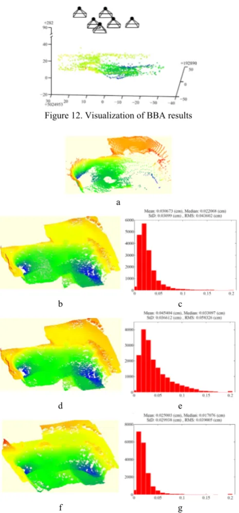
To assess the algorithms proposed in the previous section, a set of six over-lapped images from the cliff zone were selected. The initial overlapping area of the images was calculated (Figure 11), the connectivity matrix between images was determined, and the SIFT features on connected images were calculated and matched. Then, the robust motion estimation and matching was performed to determine the fundamental matrices between the stereo pair. Finally, the GCP detection was done and BBA with the method proposed in section 4.2 was performed. Figure 12 visualizes the results of BBA.
The images were once processed with Pix4D software for self-calibration, and once with our method (sections 4.1 and 4.2). Then, both of the results were input to SURE software for dense matching. Also, dense matching was performed with our algorithm (section 4.3). Then, the three obtained point clouds were compared to the ground-control, laser point cloud. It should be noted that our algorithm for dense matching is still under development. Therefore, no filtering method is still developed for removing outliers. Some of these outliers are resulted due to multi-view redundancy and some others are caused by the fact that our algorithm still lacks the aggregation of smoothness priors to the matching cost. Therefore, the disparity maps were compared with those of SURE to remove the outliers; nevertheless, in all the stereo pairs, more than 85% accordance (where the difference of calculated disparity values is less than one pixel) has been noticed between our and SURE's disparity maps. Figure 13 visualizes the generated point clouds by these tests, and the histograms of distances between each point cloud and the laser point cloud are illustrated as well. It can be noticed, that slight improvement of accuracy (about 1.5 cm) is achieved using our algorithm for motion estimation and bundle adjustment in comparison with Pix4D results. On the other hand, slight improvement of 1 cm is also observed by our dense reconstruction method in comparison with SURE.
Figure 11. The approximate fields of view of cameras
Figure 12. Visualization of BBA results
a
b c
d e
f g Figure 13. Visualization and accuracy analysis of the results. a)
laser point cloud, b) dense point cloud from SURE using our EO and IO parameters, c) histogram of distances between point clouds (b) and (a), d) dense point cloud from SURE using Pix4D EO and IO parameters, e) histogram of distances between point clouds (d) and (a), f) dense point cloud from our algorithms, g) histogram of distances between point clouds (f) and (a).
6. CONCLUSION
In this paper, we presented our approaches as well as theoretical and experimental developments for implementation and evaluation of a UAV photogrammetric system. Both aspects of data acquisition and data processing were discussed. The results obtained in comparison with the ground-control data, showed the efficient performance of our system in terms of data acquisition. The comparative results obtained from different software packages, showed the potential of our SfM The International Archives of the Photogrammetry, Remote Sensing and Spatial Information Sciences, Volume XL-1/W4, 2015
computation algorithms for improving the 3D modelling accuracy and efficiency. However, more investigation is still required, specifically for the dense matching algorithm.
ACKNOWLEDGEMENTS
This study is supported in part by grants from the: Centre de Géomatique du Québec, Fonds de Recherche Québécois sur la Nature et les Technologies, and Natural Sciences and Engineering Research Council of Canada.
REFERENCES
Ai, M., Hu, Q., Li, J., Wang, M., Yuan, H. and Wang, S., 2015. A robust photogrammetric processing method of low-altitude UAV images. Remote Sensing, 7(3), pp. 2302-2333.
Brown, D. C., 1971. Close-range camera calibration.
Photogramm Eng, 37(8), pp. 855-866.
Colomina, I. and Molina, P., 2014. Unmanned aerial systems for photogrammetry and remote sensing: A review. ISPRS J Photogramm, 92, pp. 79-97.
Francioni, M., Salvini, R., Stead, D. and Litrico, S., 2014. A case study integrating remote sensing and distinct element analysis to quarry slope stability assessment in the Monte Altissimo area, Italy. Eng Geol, 183, pp. 290-302.
Fraser, C. S., 1997. Digital camera self-calibration. ISPRS J Photogramm, 52(4), pp. 149-159.
Haala, N., Cramer, M. and Rothermel, M., 2013. Quality of 3D point clouds from highly overlapping UAV imagery. In: The International Archives of the Photogrammetry, Remote Sensing and Spatial Information Sciences, Rostock, Germany, Vol. XL-1/W2, pp. 183-188.
Herrera, G., Tomas, R., Vicente, F., Lopez-Sanchez, J. M., Mallorqui, J. J. and Mulas, J., 2010. Mapping ground movements in open pit mining areas using differential SAR interferometry. Int J Rock Mech Min, 47(7), pp. 1114-1125.
Hugenholtz, C. H., Walker, J., Brown, O. and Myshak, S., 2014. Earthwork volumetrics with an unmanned aerial vehicle and softcopy photogrammetry. J Surv Eng-ASCE, 141(1), pp. 060140031-060140035.
Ivory, J., 2012. An evaluation of photogrammetry as a geotechnical risk management tool for open-pit mine studies and for the development of discrete fracture network models. Master of Science Thesis, UCL, Australia.
Liu, P., Chen, A., Huang, Y., Han, J., Lai, J., Kang, S., Wu, T., Wen, M. and Tsai, M., 2014. A review of rotorcraft Unmanned Aerial Vehicle (UAV) developments and applications in civil engineering. Smart Structures and Systems, 13(6), pp. 1065-1094.
Manduchi, C., 1998. Stereo matching as a nearest neighbour problem. IEEE T Pattern Anal, 20(3), pp. 333-340.
McLeod, T., Samson, C., Labrie, M., Shehata, K., Mah, J., Lai, P., Wang, L. and Elder, J. H., 2013. Using video acquired from an unmanned aerial vehicle (UAV) to measure fracture orientation in an open-pit mine. Geomatica, 67(3), pp. 173-180.
Nex, F. and Remondino, F., 2014. UAV for 3D mapping applications: a review. Applied Geomatics, 6(1), pp. 1-15.
Patikova, A., 2004. Digital photogrammetry in the practice of open pit mining. In: The International Archives of the Photogrammetry, Remote Sensing and Spatial Information Sciences, Dresden, Vol. 34, Part 30, pp. 1-4.
Peng, E. and Li, L., 2010. Camera calibration using one-dimensional information and its applications in both controlled and uncontrolled environments. Pattern Recogn, 43(3), pp. 1188-1198.
Remondino, F. and Fraser, C.,2006. Digital cameras calibration methods: considerations and comparisons. In: The International Archives of the Photogrammetry, Remote Sensing and Spatial Information Sciences, Dresden, Vol. XXXVI, Part 5, pp. 266-272.
Rieke-Zapp, D., Tecklenburg, W., Peipe, J., Hastedt, H. and Haig, C., 2009. Evaluation of the geometric stability and the accuracy potential of digital cameras- comparing mechanical stabilisation versus parameterisation. ISPRS J Photogramm, 64(3), pp. 248-258.
Rothermel, M., Wenzel, K., Fritsch, D. and Haala, N., 2012. SURE: Photogrammetric surface reconstruction from imagery. In: Proceedings LC3D Workshop, Berlin, pp. 1-9.
Scharstein, D. and Szeliski, R., 2002. A taxonomy and evaluation of dense two-frame stereo correspondence algorithms. Int J Comput Vision, 47(1/2/3), pp. 7-42.
Seitz, S. M., Curless, B., Diebel, J., Scharstein, D. and Szeliski, R., 2006. A comparison and evaluation of multi-view stereo reconstruction algorithms. In: IEEE Proceedings of Computer vision and pattern recognitio, New York, pp. 519-528.
Shahbazi, M., Théau, J. and Ménard, P., 2014. Recent applications of unmanned aerial imagery in natural resource management. Gisci Remote Sens, 51(4), pp. 339-365.
Shahbazi, M., Sohn, G., Théau, J. and Ménard, P., 2015. Robust sparse matching and motion estimation using genetic algorithms. In: The International Archives of the Photogrammetry, Remote Sensing and Spatial Information Sciences, Munich, Vol. XL-3/W2, Part 30, 197-204.
Turner, D., Lucieer, A. and Watson, C., 2012. An automated technique for generating georectified mosaics from ultra-high resolution Unmanned Aerial Vehicle (UAV) imagery, based on Structure from Motion (SfM) point clouds. Remote Sensing, 4(5), pp. 1392-1410.
Turner, D., Lucieer, A. and Wallace, L., 2014. Direct georeferencing of ultrahigh-resolution UAV imagery. IEEE T Geosci Remote, 52(5), pp. 2738-2745.
Zabih, R. and Woodfill, J., 1994. Non-parametric local transforms for computing visual correspondence. Lecture Notes in Computer Science, 801, pp. 151–158.
Zhang, Y., Xiong, J. and Hao, L., 2011. Photogrammetric processing of low-altitude images acquired by unpiloted aerial vehicles. Photogramm Rec, 26(134), pp. 190-211.