MULTI-PASS APPROACH FOR MOBILE TERRESTRIAL LASER SCANNING
J. Nolan a , R. Eckels a, M. Evers b, R. Singh c, M.J. Olsen d, *
a
MNG, McMullen Nolan Group, Level 1, 2 Sabre Crescent, Jandakot, West Australia, 6164 (john.nolan, rod.eckels)@mngsurvey.com.au
b
Prairie Precision Network Inc, 5201 – 333 96 Ave NE, Calgary AB T3K 0S3, Canada, [email protected]
c
Geometronics Unit, Oregon Department of Transportation, Salem, Oregon, U.S.A. - [email protected]
d School of Civil and Construction Engineering, Oregon State University, Corvallis, Oregon, U.S.A -
Commission V, WG V/3
KEY WORDS: mobile laser scanning, control validation, multi-pass, GNSS, Control Polyline, Multipass Adjustment
ABSTRACT:
Mobile Terrestrial Laser Scanning (MTLS) has been utilised for an increasing number of corridor surveys. Current MTLS surveys require that many targets be placed along the corridor to monitor the MTLS trajectory’s accuracy. These targets enable surveyors to directly evaluate the magnitude of GNSS errors at regular intervals and can also be used to adjust the trajectory to the survey control. However, this “Multi-Target” approach (MTA) is an onerous task that can significantly reduce efficiency. It also is inconvenient to the travelling public, as lanes are often blocked and traffic slowed to permit surveyors to work safely along the road corridor. This paper introduces a “Multi-Pass” approach (MPA), which minimises the number of targets required for monitoring the GNSS-controlled trajectory while still maintaining strict engineering accuracies. MPA uses the power of multiple, independent MTLS passes with different GNSS constellations to generate a “Control Polyline” from the point cloud for the corridor. The Control Polyline can be considered as a statistically valid survey measurement and be incorporated in a network adjustment to strengthen a control network by identifying outliers. Results from a test survey at the MTLS course maintained by the Oregon Department of Transportation illustrate the effectiveness of this approach.
* Corresponding author
1. INTRODUCTION
Mobile Terrestrial Laser Scanning (MTLS) systems have been used for rail and road corridor surveys since approximately 2008 to support a wide variety of applications (Olsen et al., 2013; Williams et al., 2013). MTLS has proven to be a popular survey tool as it provides accurate, rich, 3D data efficiently and safely (Yen et al., 2011). Point cloud data resulting from a MTLS survey is initially processed in a Global Navigation Satellite System (GNSS) reference frame (WGS84 or ITRF). For most engineering projects, this data is required to be transformed into a local reference frame using transformation parameters, which are typically obtained from the measurement of survey control points identified throughout the point cloud.
In order to maximise the accuracy of the MTLS survey, all error sources need to be identified and either mitigated or eliminated. There is a large range of error sources (Glennie et al., 2007) that affect scanning – including system calibration, laser ranging accuracy, angular accuracy, Inertial Measurement Unit (IMU) drift and more. This paper focuses on the major error source that affects the positioning of the scanning vehicle itself, which is a combination of GNSS satellite multi-path, changes in satellite configuration, and geoid undulations.
Current methods for minimising satellite errors require extensive networks of targets, some of which are used to
transform the point cloud and others for validation to monitor the drift of the MTLS trajectory. In this paper, we will refer to targets generically as a mark or other object for reference, transformation control targets (TCTs) as those used to transform the point cloud between reference frames or adjust the trajectory and validation control targets (VCTs) as independent targets used solely for monitoring or validation purposes.
These “Multi-target” approaches have been adopted by public and private road agencies around the world (e.g., Caltrans 2011, Clancy 2011). Although this approach is proven to work, it has some significant disadvantages – including the substantial time required to place additional targets as well as the associated safety concerns of surveyors working on busy corridors.
This paper presents a novel “Multi-Pass” Approach (MPA), which is an alternative method of identifying MTLS trajectory drift caused by satellite errors. MPA is based on established fundamental principles of error propagation and proven surveying practices. For example, Yousif et al. (2010) describe how improved accuracy can be obtained via adjustments with 2 passes of a MTLS along a corridor. MPA further introduces the concept of a “Control Polyline” (CP), which is a 3D polyline generated parallel to the trajectory along the road from multiple independent passes of scanned data. Conceptually, the CP can be considered as a survey accurate observable – that can be
included in a network adjustment to strengthen survey networks and identify outliers.
Adopting the CP as an observation provides many advantages. These include reduced need for preplaced VCTs established to monitor MTLS trajectories, improved accuracies of surveys where a dense network of targets is unavailable, and helps identify issues with the survey control points themselves.
After describing the approach, the paper then presents results from a recent survey completed at the Oregon Department of Transport (ODOT) test range to demonstrate the capability of the MPA to deliver high accuracy survey results with MTLS.
1.1 MTLS Theory
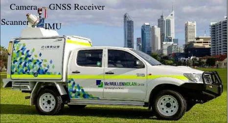
MTLS (Figure 1) is an important, efficient surveying tool consisting of three separate technologies: a laser scanner, a GNSS receiver and an inertial measurement unit (IMU) (Glennie, 2009; Graham, 2010; Puente et al., 2013). The combination of the laser scanner with these other sensors provides a point cloud containing 3D coordinates for returns from laser scanner pulses (typically hundreds of millions to billions). Measurements can be readily extracted from the point cloud and co-acquired imagery.
Figure 1. MLTS system and components
1.2 Local Reference Frame Point Cloud Transformation
The GNSS and inertial components enable each 3D point captured by the scanner to be precisely located in space. The point cloud is initially processed in the WGS84 or ITRF reference frames. Similar to GNSS-based surveys, the MTLS point cloud data is typically required in a local reference framework with orthometric heights. This transformation is typically achieved via a 2 step process.
Step 1: Transform the data from WGS84 to a local reference frame. The first step is to transform data from the GNSS system (WGS84) to a local reference frame (e.g., North American Datum, NAD83). This transformation requires “Common Control Points” to be available in both systems. The usual approach to the task requires placing well-defined TCTs along the corridor. Coordinates for the TCTs are obtained through traditional surveying techniques to tie them to established survey monuments. The targets can then be identified in the processed point cloud, providing both “local” and WGS84 coordinates.
Step 2: Convert Ellipsoidal Heights to Orthometric Heights.
The second stage of data transformation is to bring the ellipsoidal heights of the point cloud to local orthometric
heights. The relationship between these height systems is known as the geoid-spheroid undulation. The Orthometric height of all points along the corridor station can be established either by using a geoid model (e.g., NGS Geoid 12A) or incorporating control stations with known orthometric heights in the transformation process.
1.3 MTLS Error Sources
Glennie (2007) identifies several sources of error for both airborne and ground kinematic laser scanning. These include IMU drift errors, boresight angle errors, range errors, scan angle errors, lever arm measurements, and GNSS positions. In MTLS it is possible to reduce lever arm and boresight errors through calibration so that those errors are in the order of a few millimetres. For distances relatively close to the vehicle (less than 20m), the range and angular errors are relatively small. Hence, the largest error source for MTLS surveying is usually due to the inherent GNSS position error.
MTLS systems typically use a form of post-processed kinematic GNSS positioning. With most GNSS measurements, the largest component of the vertical error (when the base station is less than 10 km and ambiguities are resolved) is due to multipath. Multipath can be considered as a random error if viewed over large periods of time. However, it is temporally correlated and appears as a bias over a relative short time period. Although it is scene dependent, with high quality antennas multipath error typically has a magnitude on the order of 20 mm (1- Lau and Cross, 2007; Schön and Dilner, 2007). It is usually slow changing; however, when a satellite rises or sets into the navigation solution, the effects of multipath can change quickly. In standard surveying situations, multipath effects are mitigated by using static baselines so that the multipath error averages out over longer time periods as satellite constellations change.
2. MULTI-TARGET APPROACH TO MINIMISING
TRAJECTORY ERRORS
To achieve the highest positioning accuracies in the MTLS trajectory, these GNSS errors must be minimised. Unfortunately, the trajectory can only be independently checked at each VCT. Problems can occur between the targets – where there is no independent check of the trajectory data. While GNSS Positional Dilution of Precision (PDOP) values can be evaluated across the trajectory for an estimate to identify poor GNSS areas, they are not an independent validation source.
If the GNSS maintains lock on the satellites, the base stations are within 10 km, and the ambiguities are resolved, then the positioning error of kinematic GNSS is in the order of +/- 10 mm horizontal and +/- 20 mm vertical (1-). Under poor GNSS conditions, satellite lock can be lost and ambiguities unresolved – leading to errors of decimetres (or even metres).
MTLS manufacturers have attempted to provide a solution to these “outages” by coupling an IMU with the scanner and GNSS receiver through use of a Kalman Filter (Liu et al., 2010). The IMU can provide stable positioning information over a short time period as the vehicle moves. They are designed to “maintain lock” on position, as the scanner travels under bridges, through short tunnels, and through overhanging canopy. Although IMU’s can account for outages of several seconds of data, their position also has to be eventually updated by the GNSS receiver to avoid drift problems.
GNSS Receiver
Scanner IMU Camera
The most common approach to positioning the scanning vehicle for high accuracy engineering surveying applications, assumes that the kinematic GNSS trajectory is a weakly defined value– subject to drift caused by multipath, changing satellite configurations, and other effects. It cannot be relied upon as the source of high-accuracy positioning data and needs to be constantly monitored and checked.
The current solution to the problem of accurately defining the correct trajectory has been to provide a high density of TCTs along the corridor to correct for the drift (Figure 2).
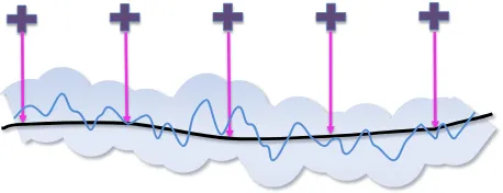
Figure 2. Sample long section showing TCTs placed on the road
• The fine blue line represents the trajectory measured from one pass of kinematic GNSS data. As this data is subject to satellite error – its uncertainty is represented by the large, wide, blue swath line – analogous to a running error bar. • The crosses represent TCTs placed along the corridor,
typically at fixed intervals
• The purple lines represent direct measurements of the local position and the point cloud position at each target • The black line represents the final corrected trajectory
along the corridor using TCTs
While techniques for placing control and performing adjustments are well defined (e.g., Clancy, 2011), the density of TCTs and VCTs required is not clearly defined. Typically, the number of additional targets required has been empirically determined – from field trials and survey experience. Manufacturers and public road agencies have developed standards, which have been proven to meet accuracy requirements (e.g., Caltrans 2011).These standards generally agree that for high accuracy, spacing of 450 m for TCTs and 150 m for VCTs is recommended. Control spacing for vertical TCTs as close as 50 m has been suggested for higher accuracy results (Soininen, 2012). However, the density of TCTs and VCTs is applied globally and does not adapt to different observing criteria (e.g., in a tunnel vs open road) as is recommended in the TRB guidelines (Olsen et al., 2013).
It should be noted that in many typical road survey applications, vertical accuracy is the most important factor (e.g., quantities, drainage, or road smoothness). An error in height by even a few centimetres can cause large errors in volume calculations for quantities (and payments) over large distances. However, GNSS measurements are naturally more accurate in the horizontal and less accurate in the vertical. This disparity is usually in the order of a factor of two and primarily due to the geometry of the satellites being above the observer and atmospheric effects on the GNSS signal propagation.
2.1 Limitations of the “Multi-Target” approach
The Multi-Target approach to controlling the trajectory of a laser scanning project has been proven to work – over a range
of scanning surveys around the world. However, the approach has significant limitations:
a) This method requires a high density of TCTs and VCTs to be established along the corridor, which necessitates a significant amount of survey work in very dangerous conditions. Placing and coordinating these targets is often the most time consuming activity in any MTLS project.
b) Regardless of how much “Monitoring” control is placed along a corridor, there is no guarantee that the MTLS trajectory has not shifted between VCTs. The only way to reduce the possibility of this error is to place even more VCTs.
c) The major assumption to this approach is that the coordinates of the TCTs and VCTs are correct. There is no independent measurement on these control point coordinates. If they are incorrect, the point cloud will be “pinned” to them by either re-calculating the final trajectory or warping the point cloud directly. Because many MTLS geo-referencing processing modules are fully automatic, black box software, these grievous errors are difficult to detect and control.
Using the Multi-Target approach, the accuracy of the final point cloud will be fully reliant on the accuracy of the control survey. The point cloud data set will not improve the accuracy of the control survey. Any errors in the control survey coordinates will directly translate to errors in the point cloud and any subsequent data extraction.
3. MULTI-PASS APPROACH
Over the last 5 years, MNG Surveys of West Australia has been developing and testing the Multi-Pass approach (MPA), which uses the strength of multiple observations and redundant data to identify and minimise errors resulting from GNSS multi-path and constellation configuration. For GNSS multipath errors, passes can be considered independent if they occur at intervals spaced at a minimal interval of fifteen minutes. (However, longer intervals are preferred when possible).
The proposed method can be employed to improve the data both horizontally and vertically, however, vertical errors are usually larger and more important to resolve. Hence, the following paragraphs describe the calculation process for correction of the vertical component of an MTLS survey.
First, a reference line is extracted from the point clouds from each pass based on a common digitized polyline. For vertical corrections, this line is usually a path along the relatively smooth road surface. The reference line is then broken into segments (e.g., 1 m). A plane is then fitted to all points that fall within a threshold (e.g., 5 cm) of the reference line for each segment of each pass. Next, the mean height is determined from the centre point of the plane for each segment. Other statistics relating to the number of points used, the quality of the line fit, and the accuracy error estimate of the trajectory for the mean of the points are also calculated.
For a 20 km reference line there may be 20,000 of these points with a single height value for each segment per pass. The weighted mean value of these points within each segment is calculated. Various weighting criteria have been used; however, the preferred method is the inverse of the trajectory error estimate corresponding to the segment. By using the trajectory weighting, any passes where the GNSS processing software
recognized that the satellite geometry (PDOP) was poor or the quality of the solution was low will have a reduced effect on the other passes.
Next the residuals of all segment heights relative to the mean value can be plotted, enabling anomalies to be removed by both visual inspection and computer algorithms taking into account the trends in the residuals along the reference line.
The final, average heights for each line segment are connected to formulate the “control polyline,” which can be considered a survey observable representing the most accurate estimate of the surface of the road along the reference line.
Once the control polyline has been established, the residuals between each segment height and the control polyline can be determined for each pass. Extracting the mean time stamp for the points contributing to this segment enables the residuals to be mapped back into the time domain of the original trajectory. The trajectories for all passes are then corrected and the entire point cloud reproduced. The result is not only a final point cloud that is more accurate but also one that is better aligned between passes than when using MTA. It should be noted that the process can be repeated using the final point cloud so that residuals can be checked as further quality control.
Similar results can also be accomplished for a horizontal adjustment. However, it requires extraction of line markings and poles; hence, it is more complex than the vertical adjustment.
The Multi-Pass approach significantly reduces the GNSS multipath error by averaging a number (n) of independent passes. In theory, statistically this reduces the error of a single pass by the square root of the number of independent passes.
k practical limitations to the error reduction that can be achieved.
3.1 Control Polyline
The concept of a survey accurate “control polyline” provides a new way of thinking about MTLS trajectories. Trajectories that are calculated from one MTLS pass are recognised to be subject to GNSS error. Even when coupled with an IMU, or constantly monitored for drift using multiple targets, they are considered a very weak observable – subject to the range of complex and unpredictable GNSS errors. It is a “best-estimate” position, which has been fixed solid at certain intervals.
The real issue, of course, is that there never really has been an easy way to monitor a kinematic GNSS line. One solution is to track the vehicle independently with a total station. Another is to run the vehicle along a known track. However, both of these options are simply not practical for real world projects.
With the high density of data provided by MTLS, it is finally possible to tie the moving survey vehicle to the fixed corridor being traversed. In most cases, it is safe to assume that any differences in the location of the road surface are due to GNSS errors rather than the road physically moving.
The strength of any survey measurements arise from two sources:
a) Independent checks – different technology used to check one’s data
b) Reliability of redundant observations – common to all surveying approaches.
The Multi-Pass approach is based on both of these concepts. A laser scanner, enables us to “see” where the scanner is heading – via millions and billions of pixels of information. The “seeing” ability in the scanner enables us to identify features in the corridor. If we run down the corridor a second time, the same features can be seen. For example, a dotted lane line in the middle of the motorway can be compared between the two scans. In the simpler case, where only the vertical error is being adjusted, only the height values of a coordinated line need to be extracted and compared along that feature.
The result of this process is the creation of a survey-accurate, 3D “handrail” along the length of the corridor, which accurately relates the point cloud of each pass. The consequences of accepting this new concept of “control polyline” are significant – representing a paradigm shift in MTLS procedures. Three of the most important consequences are:
a) There is no longer a need to place significant numbers of VCTs along the corridor to monitor GNSS drift. (Major change from state of practice).
b) The Control Polyline strengthens the network and can be used to identify errors in the control survey c) The addition of the control polyline can increase the
accuracy of the point cloud where a dense network of TCTs already exists – further improving results. In the next section, we will explore each of these paradigm shifts a little more.
3.1.1 Requirement for “Monitoring Targets” is
minimised: The “Control Polyline” provides an alternative
method to identify and minimise trajectory drift and uncertainty caused by GNSS satellite errors. Establishing the Control Polyline to a high accuracy enables significant relaxation of TCT and VCT spacing to minimise and monitor GNSS drift. The Control Polyline itself can be used to identify GNSS outliers on any particular pass of data. Once any outliers have been removed, all passes of data can be combined and averaged to provide the best trajectory solution for the entire corridor. All point cloud passes can be connected via the Control Polyline.
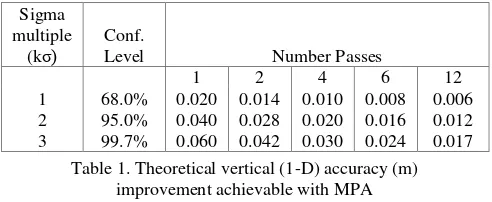
When combining independent passes of kinematic GNSS data, the accuracy improves by the square root of the number of passes (Equation 1). The table below shows an estimate of the accuracy improvement based on the number of passes (n) given the assumption of a one sigma (1-) multipath error of 20mm.
Sigma
Table 1. Theoretical vertical (1-D) accuracy (m) improvement achievable with MPA
The Control Polyline can be transformed to the local reference frame using a limited number of TCTs – placed to transform the
WGS84-based point cloud coordinate into the local reference frame. Under good GNSS conditions, experience has shown that control spaced as far as 2 km intervals can yield accuracy results better than 20 mm (2-) in the vertical.
3.1.2 Identify Errors in Control: The Control Polyline is a
survey accurate, field measurement that can be used to strengthen the entire network. The Control Polyline can be used to measure between TCTs and VCTs, to establish the coordinates of new control points and to identify if any errors in the coordinates of TCTs and VCTs.
The strength of utilising a Control Polyline can be demonstrated by considering a common scenario of a MTLS survey conducted using the traditional “multi-target” approach (MTA). In this example, target coordinates have been established at frequent intervals along the road corridor (Figure 3a). In theory, the targets should all be located on the blue line, which represents the correct location of the corridor. But, suppose the target coordinates were incorrect for one of the targets (T4) – how would this be handled by Multi-Target Approach (MTA) compared with the Multi-Pass Approach (MPA)?
Figure 3a shows a point cloud profile from one pass of MTLS (green line) along a corridor which deviates from the “true” profile (blue line) due to multipath and other errors. In this example, the coordinates surveyed for Target T4 are incorrect. Figure 3b shows how the profile would be affected using MTA to adjust the trajectory to the TCTs, resulting in distortion to conform to the incorrect coordinates of T4. The orange shading represents the positioning errors introduced to the point cloud from these faulty control values. Unfortunately, the GNSS trajectory itself provides no check on the control since it is assumed to be the problem.
(a) Initial profile from a single pass and target error (T4)
(b) Erroneous profile of a single pass following trajectory adjustment to targets using MTA
(c) Adjusted CP using MPA
Figure 3 – Example schematic of pinning trajectory to an incorrect control point (T4). The blue line represents the “true” CP, the green line represents the processed CP with associated
errors, the orange area highlights the area affected by these errors, and the stars represent locations of targets.
Figure 3c then shows the CP (green line) utilising the MPA to extract and average the profiles from multiple passes. As the CP has geometric strength from redundant observations, it will detect T4 as a major outlier. This CP provides an independent check on the target data. The surveyor now has an opportunity to check the coordinates of all control points, determine where the error has occurred, and correct the problem.
3.1.3 Increased Accuracy of a Targeted Survey Corridor.
MPA can be combined with the MTA approach to achieve even higher survey accuracies than either technique alone. In the Multi-Pass approach, the achievable accuracy increases with increased number of passes. Consequently, when processed correctly, accuracy can be increased by either reducing the control spacing, performing more passes of the road carriageway or a combination of both (Figure 4).
Figure 4. Truth Table - Multipass vs Control Spacing
4. OREGON DOT MULTIPASS TEST
4.1 Oregon DOT Test Site
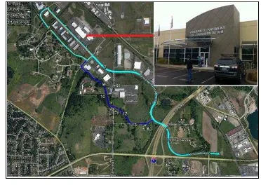
The Oregon Department of Transportation (ODOT) has established a MTLS test course near their office in Salem, Oregon. This test site (Figure 5) is a circuit approximately 3 km in length and covers a wide range of speeds and GNSS visibility. The light blue section has good GNSS visibility while the segment shown in dark blue has more challenging GNSS visibility with considerable tree cover overhanging the road.
A series of surveys have been completed to establish targets across the entire test course. High accuracy coordinates for these targets have been established through total station and levelling survey campaigns. A total of 13 targets are present across the 3 km. This was later augmented with 103 targets. For this case study, only vertical residuals are evaluated.
Figure 5. Map of the Oregon DOT MTLS test course
4.2 Data Collection
Data collection in September 2014 was completed following field methods similar to those presented in Eckels and Nolan T1
T2
T3
T4
T5
T6
(2013). A portable version of the MNG scanner system was used. This system used a Reigl VQ250 scanner and Novatel Span GNSS and IMU (Figure 1). During the survey, two base stations were used, one a permanent reference site on the roof of the Oregon DOT building, the second being located at the eastern end of the network. A subset of the network was driven 16 times. Each loop took approximately 10 minutes to complete. The vehicle was travelling at approximately 40 kph and slowing down at the key sites to 10 kph to ensure that targets were visible in the scans.
For this case study, the MTLS survey crew were initially provided with target coordinates for points 1, 3, 5, and 7 of the circuit shown in Figure 5 for use as TCTs. Oregon DOT retained the remainder of the control point coordinates as VCTs. Also, post survey, Oregon DOT established the coordinates of 103 additional VCTs along the survey route.
4.3 Processing
In all processing configurations, the data was transformed to the local reference frame using two TCTs (ODOT1 and ODOT5) located approximately 2.3 km apart. The survey was controlled using a number of stations that were established by total station traversing. From those measurements, it was estimated that the control targets were established to approximately 0.004 m (1-).
Initial trajectories were computed from the raw GNNS and inertial data using Novatel's Inertial Explorer software. Tightly coupled solutions were produced and Inertial Explorer graphs were inspected to evaluate the likely accuracy of the data. The next step was to input the raw scan data and the trajectories into a custom processing software package, NIMBUS, developed by MNG surveys to apply the MPA. A reference polyline along the route was chosen from one of the passes and the vertical data for each of the 16 polylines for these passes were extracted and plotted (Figures 6 and 7). This process provides an immediate view of the quality of the GNSS data for the MTLS solution that is not available with the analysis of GNSS by itself.
Initially all 16 passes were combined into a single point cloud for visual assessment. Overall, the data from each pass visually agreed very well. Some small segments of data on the southwest end of the project were observed to be poor in a few passes and were omitted (Table 2). After removal of the few omissions, the reference profiles from the 16 passes were averaged to obtain the CP. The CP was then transformed using the TCTs. Figure 8 plots the residuals of each pass after omission removal.
-0.10
Figure 6. Plot showing residuals of each pass relative to the distance along the CP. A small area of poor data from a few satellites can be seen at chainage 3737 to chainage 4204.
0.00
Figure 7. Error standard deviation computed during the determination of the trajectory. Note that the solution is significantly poorer due to satellite obstructions that occur after
chainage 3601. However, those errors vary substantially in magnitude between each pass.
Table 2. Periods where passes were omitted
The NIMBUS software automatically determines a weighted average for each point on the control polyline. Corrections are then determined and applied to the trajectory of each pass so that the profile extracted from the new point cloud produced will align with the CP. The mapping from the linear space of the CP to the time-related trajectories also provides a degree of smoothing of the data. The procedure is repeated and the corrected profiles for each pass are evaluated against the CP to ensure they are in agreement (Figure 9).
-0.10
Figure 8. Residuals for each pass after omissions are removed
-0.10
Figure 9. Residuals for each pass after final MPA adjustment
4.4 Target Extraction
Targets #1-12 on the test site were nails placed in the asphalt in a flat part of the road close to the curb. The targets were clearly marked with paint (Figure 10) simplifying extraction (Figure 11). Additional marks, 50100-50120 and 54026-54115 were located after the survey. For each of the 103 horizontal coordinates supplied by ODOT, the height of the road at this location was extracted from the averaged point cloud. This extracted height was then compared with the supplied height values and the residuals examined statistically.
Figure 10. Example target (L: photograph, R: point cloud)
(a) (b)
Figure 11. Sample target extraction for (a) dense and (b) sparse point cloud.
4.5 Data Analysis - MTLS and Control Error Estimation.
The prior analysis provides an internal consistency check between the various passes of MTLS data. This section describes the independent validation performed. Oregon DOT supplied horizontal coordinates and elevations from an additional 103 VCTs around the network that were located using total station measurements. Initial results showed a number of outliers (Figure 12).
-0.04
Figure 12. Comparison of residuals of control polyline to initial control point coordinates
These issues were analysed by Oregon DOT and resolved. Of these four outliers, the two largest were due to erroneous coding where the point was not on the pavement, and the two others were shot by the field crew at a distance that was longer than normal. These smaller errors, in particular, were a good example of the magnitude of errors that can be detected using the CP and redundant data provide by MPA. An analysis of the
remaining residuals (Figure 13) was then made with the statistical results shown in Table 3. The final RMS error for the data comparison is 6 mm.
Figure 13. Plot of residuals of MTLS data from the average of 16 passes compared with total station data
Statistic Residual (m)
Table 3. Statistical analysis of vertical residuals presented in Figure 13 comparing point cloud measurements with the total
station coordinates. (n = 108).
To analyse the degree of improvement of each pass when using multiple passes, the 16 passes of the CP were divided into subsets of 1, 2, 4, 8, and 16 passes and reprocessed. For each solution, a CP was determined, the elevations of the 103 control coordinates were extracted from the averaged point cloud, and those values were compared to the total station values. For each subset, a standard deviation of the residuals were calculated and shown in Table 4.
Table 4. Measured standard deviation errors based on number of passes
5. DISCUSSION
The results show that by carefully combining the accuracy from multiple passes of a MTLS system, higher accuracy point clouds can be generated compared with the results from a single pass. This higher accuracy was obtained without the need to use multiple TCTs at close range. The results indicate that the much larger separations between TCTs and VCTs can be adopted while still maintaining survey accuracy. While current standards (e.g., Caltrans) for MTLS dictate that control must be placed every 150 m, this case study shows that an accuracy of 0.007 m (1-) was achievable with TCTs spaced farther than 2 km apart.
The analysis in Table 4 agrees very well with the theoretical values computed in Table 1. However, this analysis also highlights a key problem when trying to validate measurements over several kilometres to an accuracy of better than a few ppm. That is, the errors inherent in the measurement of the control
system are similar in magnitude to the measurement errors that we are trying to detect in the new method of using MTLS.
The common practice of placing dense control and then warping a single MTLS pass to fit these points significantly reduces efficiency. The cost of placing control on busy roads and employing traffic control staff to close lanes is high. The trial has shown that similar (or better) accuracy can be achieved by relatively quickly collecting additional data passes in the field, which significantly reduces the time of survey, is cost efficient, and is safer for surveyors and the travelling public.
MPA also offers additional advantages in addition to accuracy. The denser point cloud resulting from combining multiple scans provides a higher resolution dataset. Additionally, combining point cloud data from several passes reduces the data gaps caused by passing traffic, parked cars, etc. Because each data pass occurs at a different time, the possibility of the same obstruction being at the same place is reduced.
5.1 Caveat
It should be noted that for the MPA method to work effectively, the GNSS solution for the majority of passes must be of reasonable quality. If the GNSS solution is poor (i.e., inertial only for long periods or potential incorrect bias solutions), then these errors will bias the solution of MPA just as they will with multi-target approach. However, the advantage of MPA is that it provides QA tools to help identify this poor data.
Use of a geoid model will also introduce a degree of error in orthometric heights. For the study area, NGS (2014) estimates 4-5 cm @95% confidence for Geiod12A. This geoid error varies spatially and can increase with project distance. For this reason some transformation control targets are still required; however using MPA, these can be placed at a greater spacing than required in traditional methods.
6. CONCLUSIONS
The standard method in practice today (MTA) for high accuracy road corridor surveys is to use dense networks of local targets to control MTLS surveys. This method is conceptually simple to implement; however, it is also very inefficient and poses a variety of practical problems
The MPA is an effective alternative whereby the detail contained in the point cloud is made more accurate by combining it with the statistical addition of independent, redundant measurements. As the road surface is unlikely to have shifted in the short time between passes, a more accurate road surface can be derived from the sum of multiple scans than from any of the individual scans by themselves. From the combined point clouds from each pass, a new observable called the "control polyline" can be derived and used to augment existing control networks along with more traditional observations.
MPA, for the first time, provides a simple method to examine the errors in kinematic GNSS. When processed appropriately, the full accuracy of the GNSS system can be enhanced by using multiple scans. Utilising MPA, allows for a significant reduction of validation targets – leading to increased workplace safety, time savings, increased accuracy and/or reduced costs. Furthermore, the GNSS/inertial controlled point cloud can be utilised as a measurement in its own right both strengthening control networks and identifying outliers.
Ultimately, MTA and MPA are both useful methods for MTLS. For optimum project deliveries, the ability to use the right combination of both methods will be essential.
ACKNOWLEDGEMENTS
The authors would like to thank Daniel E Wright and staff at the Oregon DOT for providing control coordinates for the test network. MNG would also like to thank Wayne Cannell, Greg Myers and staff at the department of Main Roads, Western Australia and Neville Janssen, Tony Kirchner, John E. Allsop and others at Transport and Main Roads, Queensland for their support and assistance in pioneering new methods for the use of mobile scanning in Australia.
REFERENCES
California Department of Transportation, 2011. Terrestrial Laser Scanning Specifications. In Surveys Manual, CalDOT: Sacramento, CA, USA, 2011, Chapter 15.
Clancy, S., 2011. The importance of Applied Control. LIDAR Magazine, Vol. 1, pp. 26–30.
Eckels R. and Nolan J., 2013 Mobile Laser Scanning: Field methodology for achieving the highest accuracy at traffic speed,
Proc. of Association of Public Authority Surveyors Conference (APAS2013), Canberra, Australia, 12-14 March, pp. 218-230.
Glennie, C., 2007. Rigorous 3D error analysis of kinematic scanning LIDAR systems. J. Appl. Geod., Vol. 1, pp. 147–157. Glennie, C., 2009, Kinematic terrestrial light-detection and ranging system for scanning. Transp. Res. Rec. Vol. 2105, pp. 135–141.
Graham, L., 2010. Mobile mapping systems overview.
Photogramm. Eng. Remote Sens. Vol. 76, pp. 222–228. Lau, L., and Cross, P., 2007. Investigations into phase multipath mitigation techniques for high precision positioning in difficult environments, J. of Nav., Vol. 60(3), pp. 457-482.
Schön, S., and Dilner, F., 2007. Challenges for GNSS-based high precision positioning – some geodetic aspects, 4th
Workshop on Positioning, Navigation, and Communication.
Soininen, A., 2012. Mobile Accuracy and Control, How much control do we need? https://www.terrasolid.com/ download/presentations/2012/mobile_accuracy_and_control.pdf
National Geodetic Survey, 2014. Geoid 12A Estimated Accuracy Map, (http://www.ngs.noaa.gov/GPSonBM/maps/ GEOID12A_Accuracy.png).
Olsen, M.J., Roe, G.V., Glennie, C., Persi, F., Reedy, M., Hurwitz, D., Williams, K., Tuss, H., Squellati, A., Knodler, M. 2013. Guidelines for the Use of Mobile LIDAR in Transportation Applications, TRB NCHRP Final Report 748, TRB: Washington, DC, USA, 250 pp.
Yen, K.S., Ravani, B., and Lasky, T.A., 2011. LiDAR for Data Efficiency, AHMCT Research Center: Davis, CA, USA.
Yousif, H., Li, J., Chapman, M., and Shu, Y., 2010. Accuracy enhancement of terrestrial mobile lidar data using theory of assimilation. Int. Arch. Photogramm. Remote Sens. Spat. Inf. Sci. Vol. 38, pp. 639–645