FOREST STAND SEGMENTATION USING AIRBORNE LIDAR DATA
AND VERY HIGH RESOLUTION MULTISPECTRAL IMAGERY
Cl´ement Dechesne, Cl´ement Mallet, Arnaud Le Bris, Val´erie Gouet, Alexandre Hervieu
IGN / SRIG - Laboratoire MATIS - Universit´e Paris Est - Saint-Mand´e, FRANCE [email protected]
Commission III, WG III/2
KEY WORDS:lidar, multispectral imagery, fusion, feature extraction, supervised classification, energy minimisation, forest stand delineation, tree species.
ABSTRACT:
Forest stands are the basic units for forest inventory and mapping. Stands are large forested areas (e.g.,≥2 ha) of homogeneous tree species composition. The accurate delineation of forest stands is usually performed by visual analysis of human operators on very high resolution (VHR) optical images. This work is highly time consuming and should be automated for scalability purposes. In this paper, a method based on the fusion of airborne laser scanning data (or lidar) and very high resolution multispectral imagery for automatic forest stand delineation and forest land-cover database update is proposed. The multispectral images give access to the tree species whereas 3D lidar point clouds provide geometric information on the trees. Therefore, multi-modal features are computed, both at pixel and object levels. The objects are individual trees extracted from lidar data. A supervised classification is performed at the object level on the computed features in order to coarsely discriminate the existing tree species in the area of interest. The analysis at tree level is particularly relevant since it significantly improves the tree species classification. A probability map is generated through the tree species classification and inserted with the pixel-based features map in an energetical framework. The proposed energy is then minimized using a standard graph-cut method (namely QPBO withα-expansion) in order to produce a segmentation map with a controlled level of details. Comparison with an existing forest land cover database shows that our method provides satisfactory results both in terms of stand labelling and delineation (matching ranges between 94% and 99%).
1. INTRODUCTION
Fostering information extraction in forested areas, in particular at the stand level, is driven by two main goals : statistical inven-tory and mapping. Forest stands are the basic units and can be defined in terms of tree species or tree maturity. From a remote sensing point of view, the delineation of the stands is a segmenta-tion problem. In statistical forest inventory, segmentasegmenta-tion is help-ful for extracting statistically meaninghelp-ful sample points of field surveys and reliable features (basal area, dominant tree height, etc.) (Means et al., 2000, Kangas and Maltamo, 2006). In land-cover mapping, this is highly helpful for forest database updating (Kim et al., 2009). Most of the time, for reliability purposes, each area is manually interpreted by human operators with very high resolution geospatial images. This work is extremely time con-suming. Furthermore, in many countries, the wide variety of tree species (around 20) makes the problem harder.
The use of remote sensing data for the automatic analysis of forests is growing, especially with the synergetical use of air-borne laser scanning (ALS) and optical imagery (very high reso-lution multispectral imagery and hyperspectral imagery) (Torabzadeh et al., 2014).
Several state-of-the-art papers on automatic forest stand delin-eation with Earth Observation data have been already published. First, it can be achieved with a single remote sensing source. A stand delineation technique using hyperspectral imagery is pro-posed in (Leckie et al., 2003). The trees are extracted using a valley following approach and classified into 7 tree species (5 coniferous, 1 deciduous, and 1 non-specified) with a maximum likelihood classifier.
A stand mapping method using low density airborne lidar data is proposed in (Koch et al., 2009). It is composed of several steps of feature extraction, creation and raster based classification.
For-est stands are created by grouping neighbouring cells within each class. Then, only the stands with a pre-defined minimum size are accepted. Neighbouring small areas of different forest types that do not reach the minimum size are merged together to a forest stand.
The forest stand delineation proposed in (Sullivan et al., 2009) uses low density airborne lidar for an object-oriented image seg-mentation and supervised classification. Three features (canopy cover, stem density, and average height) are computed and raster-ized. The segmentation is performed using a region growing ap-proach. Spatially adjacent pixels are grouped into homogeneous discrete image objects or regions. Then, a supervised discrimi-nation of the segmented image is performed using a Battacharya classifier, in order to define the maturity of the stands (i.e., the labels correspond to the maturity of the stands).
Lidar point clouds
VHR multispectral image Features
Classification Segmentation based on regularisation Individual trees
Training set
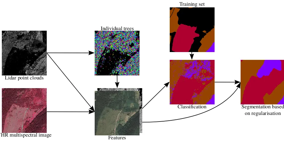
Figure 1. Flowchart of the proposed method. Colour codes :Douglas,spruce,woody heathland.
TSI, FDI and SPI features. Forest stand refinement is achieved with a seeded region growing approach. This method provides a coarse-to-fine segmentation with relatively large stands.
Other methods using the fusion of different types of remote sens-ing data have also been developed. Two segmentation methods are proposed in (Lepp¨anen et al., 2008) for a forest composed of Scots Pine, Norway Spruce and Hardwood. A hierarchical seg-mentation on crown height model and a limited iterative region growing approach on composite of lidar and Coloured Infra-Red (CIR images). The second method proposes a hierarchical seg-mentation on crown height model where each image object is connected both to upper and lower level image objects. This al-lows to consider final segments onto the finest segmentation level, like recognizing individual trees in the area.
The analysis of the lidar and multispectral data is performed at three levels in (Tiede et al., 2004). The first level represents small objects (single tree scale; individual trees or small group of trees) that can be differentiated by spectral and structural characteristics using a rule-based classification. The second level corresponds to the stand. It is built using the same classification process which summarizes forest-development phases by referencing to small scale sub-objects at level 1. The third level is generated by merg-ing objects of the same classified forest-development into larger spacial units. This method produces a mapping guide in order to assess the forest development phase (i.e., the labels do not corre-spond to tree species).
Since the stands are the basic unit for statistical inventory some segmentation methods for that purpose have been developed in (Diedershagen et al., 2004) and (Hernando et al., 2012).
With respect to existing methods, it appears that there are no for-est stand segmentation method based on tree species that can sat-isfactorily handle a large number of classes (>5). It also appears that working at the object level (usually tree level), in order to dis-criminate tree species, produces better the stand segmentation re-sults. Several methods for tree species classification at tree level have been investigated in (Heinzel and Koch, 2012), (Leckie et al., 2003) and (Dalponte et al., 2015a). However, is likely to be
imprecise, resulting in an inaccurate tree classification. However, the output of the classification of tree species at tree level may be used for forest stand delineation.
In this paper, a method for species-stand segmentation is pro-posed. The method is composed of three main steps. Features are first derived at the pixel and at the tree level. The trees are extracted using a simple method, since this appears to be suffi-cient for subsequent steps. A classification is performed at the tree level as it significantly improves the discrimination results (about 20% better than the pixel-based approach). This classifi-cation is then regularised through an energy minimisation. The regularisation, performed with a graph-cut method, produces ho-mogeneous tree species areas with smooth borders.
The paper is structured as follows : the method is presented in Section 2. In this section, the feature extraction, the classification and the regularisation are presented. The method is evaluated in Section 3. The dataset is presented followed by the results of the method. Finally, a conclusion is proposed in Section 4. with a summary of the method and the forthcoming improvements of the method.
2. METHOD
The proposed method is composed of three main steps. First, 12 features are derived from the ALS and multispectral data (Sec-tion 2.1). They are computed at the pixel level as it is needed for the energy minimisation. They are also computed at the object level (trees); the features are more consistent at the tree level and significantly improve the accuracy of the classifiers. Then, the classification of tree species is performed using standard classi-fiers (Section 2.2). Finally, a smooth regularisation based on an energy minimisation framework is carried out in order to obtain the final segments (Section 2.3). A summary of the method is presented in Figure 1.
2.1 Feature computation
features will be computed both at the pixel and object level. For the lidar data, features are computed at the point level and then rasterized using a pit-free method (see Section 2.1.4) at the res-olution of the multispectral image. Multispectral features are also computed at the pixel level. The pixel-based feature maps are merged in order to create a global pixel-based feature map. Then, an object-based feature map is created using the pixel-based feature map and the extracted trees. The feature putation method is summarized in Figure 2. The various com-puted features are presented in Table 3 and described in Sec-tions 2.1.2, 2.1.3 and 2.1.4.
Pixel-based
Figure 2. Feature extraction flowchart.
Lidar features Multispectral features
CHM Reflectance in
Vegetation density based on the red band local tree top Reflectance in Vegetation density based on the green band ratio of ground points Reflectance in over non-ground points in the blue band
Planarity Reflectance in
Scatter the near-infra-red band
NDVI DVI RVI
Table 3. Computed features both at pixel and object levels.
2.1.1 Tree extraction. Recently, tree delineation has been extensively investigated in the literature, see for instance (Dalponte et al., 2015b) and (Tochon et al., 2015) for the latest existing methods. Many methods exist and it is well known that there is no golden standard for individual tree crown delineation (Kaartinen et al., 2012). Here, accurate tree delineation is not the aim of the proposal but a geometrically meaningful over-segmentation technique for object-based image analysis and feature computation. Consequently and for scalability purposes, a simple method with few parameters is sufficient.
A coarse method is adopted: the tree tops are first extracted using a local maxima filter (from experiments, a 5 meter radius filter appears to be the best choice on the considered dataset). Only the points above 5 meters are retained. Points are aggregated to the tree tops according to their relative height to the tree top and distance from the closest point from the tree. An example of our
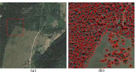
tree delineation is presented in Figure 4.
(a) (b)
Figure 4. Result of the tree delineation. (a) Orthoimage (1 km2 ): the red square corresponds to the sub-area where the tree delin-eation results (b) are presented.
2.1.2 Point-based lidar features. Lidar-derived features (such as vegetation density, scatter and planarity) require a con-sistent neighbourhood for their computation. For each lidar point, 3 cylindrical neighbourhoods are used (1 m, 3 m and 5 m radius). Two vegetation density features are computed; one based on the number of local maxima within the neighbourhoods and an other related to the number of non-ground points within the neighbour-hoods (ground points were previously determined by filtering). The scattersand the planaritypare computed as follow (Wein-mann et al., 2015) : within the cylindrical neighbourhoods of radiusr.
4 features are extracted during this step. These features provide information about the structure of the forest that is related to species it is composed of.
Some other features such as percentiles can be computed using the same method as they are known to be relevant for tree species classification (Dalponte et al., 2014, Torabzadeh et al., 2015). They are not used here in order to reduce the complexity of the method and the computation times.
2.1.3 Pixel-based multispectral features. The original 4 bands from the image are kept and considered as multispectral features. The Normalized Difference Vegetation Index (NDVI) (Tucker, 1979), the Difference Vegetation Index (DVI) (Bacour et al., 2006) and the Ratio Vegetation Index (RVI) (Jordan, 1969) are computed as they are relevant vegetation indicators. These indicators provide more information about the species than the original bands alone. Finally, the pixel-based multispectral features map is composed of 7 features. Some other feature could be processed such as texture features but were also not considered in this study order to reduce the complexity of the method and the computation times.
Orthoimage (1km²) RF-p SVM-p RF-o SVM-o
Figure 5. Classification results; comparison of the classifiers and of the pixel and object based approach. Species colour codes :beech, chestnut,robinia,oak,Scots pine,Douglas,spruce,woody heathland,herbaceous formation.
2.1.5 Object-based feature map. The pixel-based multi-spectral and lidar maps are merged so as to obtain a pixel-based feature map. Then, an object-based feature map is created using the individual trees and the pixel-based feature map. The value of a pixel belonging to a tree in the object-based feature map is the mean value of the pixels belonging to that tree. Otherwise, the pixel keeps the value of the pixel-based feature map (see Figure 6). In this paper, only the mean value of the pixels within the tree is envisaged but one can also consider other statistical values (minimum, maximum, percentiles etc.).
Other features could be derived from the lidar cloud point at the object-level. For instance, an alpha-shape can be performed on the individual trees and a penetration feature can be derived as it can help classifying tree species (some species let the lidar penetrate the canopy). However, low point densities (1-5 points/m2
) compatible with large-scale lidar surveys are not sufficient in order to derive a significant penetration indicator.
Pixel-based density map Object-based density map
Figure 6. Difference between the pixel-based feature map and the object-based feature map of the sub area of Figure 4(b). Black color corresponds to low vegetation density area and white color to high vegetation density area.
2.2 Tree species classification
The classification is performed using a supervised classifier in order to discriminate tree species provided by the training set. Two classical classifiers are used and their accuracies will be compared ; the Random Forest (RF), implemented in OpenCV (Bradski and Kaehler, 2008) and the Support Vector Machine (SVM) with radial basis function kernel, implemented in LIB-SVM (Chang and Lin, 2011). Two strategies are carried out; one on the object-based feature map and the other on the pixel-based feature map. The 12 features (lidar and multispectral) are used for the classification. 4 scenario are considered: RF on the pixel-based feature map (RF-p), SVM on the pixel-based feature map (SVM-p), RF on the object-based feature map (RF-o), and SVM on the object-based feature map (SVM-o). For each classifier, 1000 samples per class are randomly selected
from the manually delineated forest stands in order to train the model. The optimisation of the SVM parameters is carried out through a cross-validation. The outputs of the classification are a classification map and a probability map (probabilities of belonging to the class for each pixel/object). This probability map is one of the input for the regularisation step.
The classification results are presented for a 1 km2
mountainous forest area in Figure 5. The accuracy is obtained by comparing classified pixel to all labelled pixel in the manual delineation. It appears clearly that the pixel-based approach leads to noisy label maps. Conversely, even if the tree extraction is approximative, the object-based feature map leads to a more spatially consistent classification. One can also see that both classifiers are equivalent in terms of discrimination results as stated in other studies (Du et al., 2012). In terms of accuracy, the RF-p performs the worse with 66% of well classified pixels. The SVM-p performs slightly better with 73% of correctly classified pixels. The SVM-o and RF-o perform the best with respectively 89% and 90% of well classified pixels. These same kind of results are observed on the other zones.
2.3 Regularisation
As shown in Figure 5, the classification is not sufficient to ob-tain homogeneous areas with smooth borders. Regularising the classification at the pixel level, through an energy minimisation framework, appears to be a good method to overcome this prob-lem.
The energy model is a probabilistic graph taking into account the probabilities of belonging to the classes and the pixel-based fea-ture mapA. For an imageIand a classificationC, the energyE is formulated as follows :
E(I, C) =X u∈I
Edata(C(u)) +γ X u,v∈N
Ebinary(C(u), C(v)),
(3) with
γ∈[0,∞[,
Edata(C(u)) = f(P(C(u))), Ebinary(C(u) =C(v)) = 0,
Ebinary(C(u)6=C(v)) = V(u, v).
values of the features of the pixeluare different from the one of its neighbour. The total energy expresses how good the pixel is classified and how close its features are from the ones of its neighbours.
Some other methods such as Conditional Random Fields (CRF) could be envisaged for the expression of the energy (Volpi and Ferrari, 2015), Ebinary would then be expressed relatively to all the pixel within the image instead of only the 8-connectivity neighbourhood. They were not adopted here.
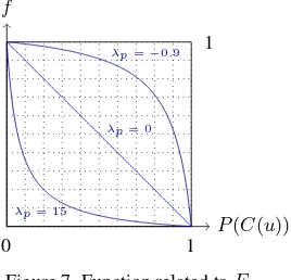
2.3.1 Data term. The functionfrelated toEdatais the fol-lowing:
f(x) = 1−x
λpx+ 1, (4)
x∈[0,1], λp∈]−1,∞[.
This function allows to control the importance we want to give to the raw classification step (see Figure 7). The moreλpis close to−1, the more the value of the energy will be important, even if the pixel has a high probability to belong to the class. Conversely, the greaterλpis, the less the value of the energy will be impor-tant, even if the pixel has a low probability to belong to the class. This parameter is highly relevant in case of complex tree species discrimination and a large number of misclassified pixels.
P(C(u))
Figure 7. Function related toEdata.
2.3.2 Regularisation term. The regularisation term controls the value of the energy according to the value of the features within the 8-connexity neighbourhood. Two pixels with differ-ent class labels but with close feature values are more likely to belong to the same class than two pixels of different classes and different feature values. The value of the energy should be near to 0 when the feature values are close and increase when they are different. The binary energy is expressed as follows:
∀i λi∈[0,∞[,
whereiis related to a feature.
λis a vector of length equal to the number of computed features. This vector allows to assign different weights to the different features. Ifλi = 0, the feature will not be taken into account in the regularisation process. The moreλiis important, the more a small difference in the feature value will lead to an increase of the energy. The features are of different types (height, reflectance, density, etc.), it is therefore important to have a term in[0,1]for each feature, even if they do not have the same range. In the next experiment,λiis set to 1 for the 4 multispectral bands, NDVI, height andλiwas set to 0 for the other features. These 6 features were arbitrarily chosen. Additional investigation on the value of theλiwill be conducted in the future.
2.3.3 Energy minimisation. The energy minimisation is performed by quadratic pseudo-boolean optimization (QPBO)
method withα-expansion. The QPBO is a popular and efficient graph-cut method as it efficiently solve energy minimization problems by constructing a graph and computing the min cut (Kolmogorov and Rother, 2007). Theα-expansion allows to deal with multiclass problems (Kolmogorov and Zabih, 2004).
The effect ofγis presented in Figure 8. Whenγ= 0, the energy minimisation has no effect; the most probable class is attributed to the pixel. When γ 6= 0, the result is more homogeneous. One can also see that the border of the homogeneous zones are smoother whenγincreases. However, the greater γis, the smaller area might be merged with the larger ones. In order to have a good compromise between smooth borders and consistent areas,γshould be in[1,3].
3. EVALUATIONS
In this section, the test area is first presented. The results are then discussed and the computation times of our method are presented.
3.1 Data
The test area is a mountainous forest in the East of France. 8 areas of 1 km2
composed of a wide range of tree species are processed (see Figure 13). The multispectral images have 4 bands; 430-550 nm (blue), 490-610 nm (green), 600-720 nm (red) and 750-950 nm (near infra-red) at 0.5 m spatial resolution. The average point density for airborne lidar data is 3 points/m2
. Data was acquired under leaf-on conditions.
The lidar data was pre-processed: the point cloud was filtered in order to remove outliers and determine ground points. The ground points were extrapolated so as to derive a Digital Terrain Model (DTM) at 1 m resolution. Then, the DTM was subtracted from the point cloud since a normalized point cloud is necessary in order to perform the coarse tree delineation.
The multispectral images and ALS data are perfectly co-registered but were acquired at different epochs. This may imply some minor errors that have no real impact on our results. The polygons delineated by photo-interpreters were used in order to train the classifiers and also to evaluate the results. Only the polygons containing at least 75% of a species were used for the classification. The polygons of natural bare soils (woody heathland and herbaceous formation) are also used for the classification. As it is based only on species, the ground truth used will only cover a small part of the area (the test areas contain also stands of mixed species). Each of the 8 areas were processed separately. The 40 polygons cover only a small part of the areas and thus, only few species are available for the classification. Additionally, stands borders resulting from the methods might not match with the border of the polygons.
3.2 Results
Orthoimage (1km²)
Figure 8. Effect of the smoothing parameterγon the segmentation. See Figure 5 for the colour codes.
regularisation with the ones from the manual delineation ranges between 94% and 99% (results are presented for each area in Table 9),compared to a matching≤90% after classification. The matching ratio is obtained by comparing the well classified pixel to all labelled pixel in the manual delineation. The improve-ments also concern the homogeneity of the segimprove-ments delineated automatically. Segmentation results are much less noisy than the classification results. The errors occur at the borders between the delineated stands. There are two kinds of errors: (i) the ones due to the uncertainty of the borders, and (ii) the ones due to misclassification (see Figure 10). The uncertainty of the borders is related to the generalisation of our ground truth. The manual and the automatic delineation are performed at the same spatial resolution, this implies inevitable small shifts at the borders of the stands.
Segmentation accuracy Area 1 98.7% Area 2 99.0% Area 3 99.6% Area 4 98.2% Area 5 97.1% Area 6 98.7% Area 7 94.2% Area 8 99.3%
Table 9. Matching of the polygons obtained after regularisation with the ones from the manual delineation.
(a) (b)
Figure 10. Differences between the human delineation and our segmentation. In (a), white is a correct classification of species, black is a wrong classification and grey is unknown (i.e., no polygon). In (b), erroneous areas are superposed on the orthoim-age, blue corresponds to errors due to the uncertainty of the bor-der, red corresponds to misclassification.
Figure 11 shows how well our method fits to the forest borders. Some borders are modified and are more consistent visually.
Stands that were not delineated by human operators are found with our method. However, some forested areas are merged to non-forested areas. These errors can easily be explained ; the ground truth contains wrong data such as trees in non-forested areas, that leads to misclassification. This example also shows that the open forest (canopy cover between 10% and 40%) raises problems as they are merged to non-forested areas. The case of open forest should be considered separately (see Section 4.).
(a) (b)
2 2 3
1 2
2 4
5 2
2 3
1 2
2 4
5
4 4
Figure 11. Delineation of the stands (in blue) superposed to the IRC orthoimage (area 7 in Figure 13). (a) Delineation by human operator. (b) Automatic delineation. 1: training error,2: new forest stands,3: new border more consistent visually,4: forested areas merged with herbaceous formation,5: open forest (canopy cover between 10% and 40%) labelled as woody heathland.
3.3 Computation times
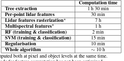
The computation times, averaged over the 8 zones, are summa-rized in Table 12. The most time consuming step is related to the processing of the ALS data, and especially the computation of the feature. However, the code could be improved in order to reduce the computation times. For the classification, the RF performs faster than the SVM and, since the tree species classification are close for both classifiers (see Section 2.2), the use of the RF classifier more relevant.
Computation time Tree extraction 1 h 30 min Per-point lidar features 30 min Lidar features rasterization⋆ 7 h Multispectral features⋆ 1 h
RF (training & classification) 2 min SVM (training & classification) 15 min
Regularisation 10 min
Whole algorithm ∼10 h
⋆computed both at pixel and object levels at the same time.
The code for feature computation has not been optimized.
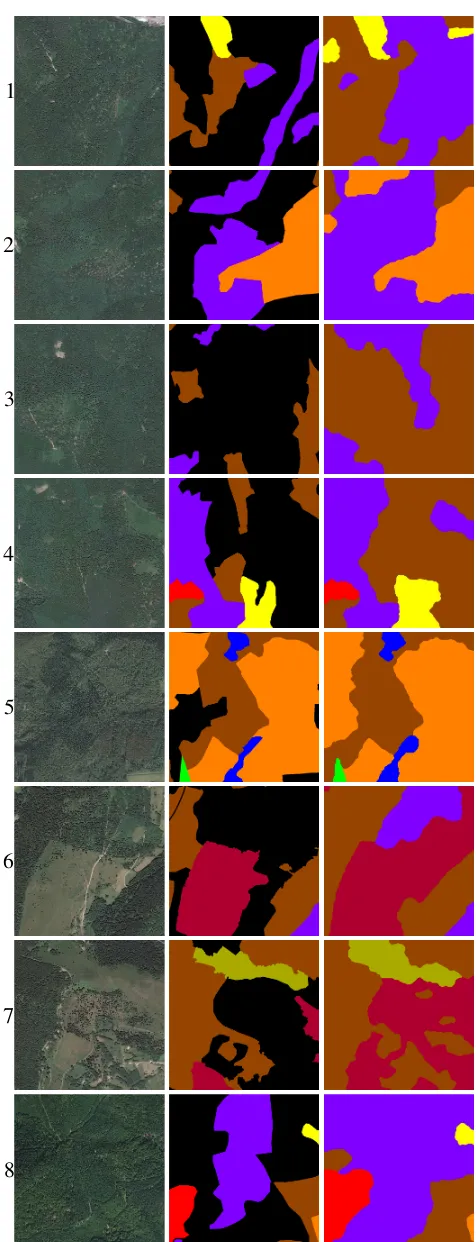
1
2
3
4
5
6
7
8
Figure 13. Results of the method for 8 areas of 1 km2
. The first column contains the orthoimage of the areas, the second contains the polygons delineated by photo-interpreters (black color cor-responds to unlabelled data) and the third column contains the result of the regularisation. See Figure 5 for the colour codes.
4. CONCLUSION 4.1 Discussion
In this paper, a 3-step method for forest stand delineation according to tree species was proposed. The fusion of ALS data and multispectral images produces good results since both remote sensing modalities provide complementary observations. The final segments have a good matching with the segment delineated by human operators. The method relies on the computation of lidar and multispectral features at different levels (pixel and tree) for a supervised classification of tree species. Good discrimination scores are already obtained with standard features and classifiers, which is a strong basis for accurate delineation. A regularisation was then performed through an energy minimisation in order to obtain homogeneous areas in terms of species and smooth borders. This energy is formulated according to both classification results and feature values. It is highly helpful in order to control the level of details required for the segments, which depends on the inventory or land-cover database specifications.
4.2 Forthcoming improvements
A first improvement is on the feature computation; some other features could be extracted in order to improve the classification on both multispectral and ALS data (Torabzadeh et al., 2015). Investigation should also be conducted about the energy formu-lation and especially the choice of the relevant features and the automatic tuning of their relatedλi. Some experiment should also be conducted to see the effect ofλp on the result of the regularisation and how it can be automatically tuned.
More experiments should also be conducted in order to assess the benefit of the object-level classification on the final result. Since the aim is to delineate forest stands according to tree species, the use of hyperspectral images might be interesting so as to obtain more information about the species. Some other vegetation indices can also be derived from hyperspectral data. The use of higher density ALS data (∼10 pts/m2
) might also improve the results of the method; trees would be extracted more precisely and some new structural features could be derived. For land-cover mapping, the energetical framework will be mod-ified in order to be able to retrieve other levels of hierarchical forest databases, with the same inputs (trees and species): mixed forests (not any of a single tree specie cover>75%) and open forests (canopy cover between 10% and 40%).
Finally, during the training step of the classifiers, some pixels might not belong to the species of the concerned polygon (since polygons are pure at least at 75%) and only few classes are available. The model should be trained on a larger area and an unsupervised classification should be conducted in order to remove outliers and better tailor the training set.
REFERENCES
Bacour, C., Br´eon, F.-M. and Maignan, F., 2006. Normalization of the directional effects in NOAA–AVHRR reflectance measure-ments for an improved monitoring of vegetation cycles. Remote Sensing of Environment 102(3), pp. 402–413.
Bradski, G. and Kaehler, A., 2008. Learning OpenCV: Computer vision with the OpenCV library. ” O’Reilly Media, Inc.”.
Dalponte, M., Ene, L. T., Witte, C., Marconcini, M., Gobakken, T. and Næsset, E., 2015a. Semi-supervised SVM for individual tree crown species classification. ISPRS Journal of Photogram-metry and Remote Sensing 110, pp. 77–87.
Dalponte, M., Ørka, H. O., Ene, L. T., Gobakken, T. and Næsset, E., 2014. Tree crown delineation and tree species classification in boreal forests using hyperspectral and ALS data. Remote Sensing of Environment 140, pp. 306–317.
Dalponte, M., Reyes, F., Kandare, K. and Gianelle, D., 2015b. Delineation of individual tree crowns from ALS and hyperspec-tral data: a comparison among four methods. European Journal of Remote Sensing 48, pp. 365–382.
Diedershagen, O., Koch, B. and Weinacker, H., 2004. Automatic segmentation and characterisation of forest stand parameters us-ing airborne lidar data, multispectral and fogis data. International Archives of Photogrammetry, Remote Sensing and spatial Infor-mation Sciences 36(8/W2), pp. 208–212.
Du, P., Xia, J., Chanussot, J. and He, X., 2012. Hyperspectral re-mote sensing image classification based on the integration of Sup-port Vector Machine and Random Forest. In: IEEE International Geoscience and Remote Sensing Symposium, pp. 174–177.
Heinzel, J. and Koch, B., 2012. Investigating multiple data sources for tree species classification in temperate forest and use for single tree delineation. International Journal of Applied Earth Observation and Geoinformation 18, pp. 101–110.
Hernando, A., Tiede, D., Albrecht, F. and Lang, S., 2012. Spatial and thematic assessment of object-based forest stand delineation using an OFA-matrix. International Journal of Applied Earth Ob-servation and Geoinformation 19, pp. 214–225.
Jordan, C. F., 1969. Derivation of leaf-area index from quality of light on the forest floor. Ecology 50(4), pp. 663–666.
Kaartinen, H., Hyypp¨a, J., Yu, X., Vastaranta, M., Hyypp¨a, H., Kukko, A., Holopainen, M., Heipke, C., Hirschmugl, M., Mors-dorf, F. et al., 2012. An international comparison of individual tree detection and extraction using airborne laser scanning. Re-mote Sensing 4(4), pp. 950–974.
Kangas, A. and Maltamo, M., 2006. Forest inventory: method-ology and applications. Vol. 10, Springer Science & Business Media.
Khosravipour, A., Skidmore, A. K., Isenburg, M., Wang, T. and Hussin, Y. A., 2014. Generating pit-free canopy height mod-els from airborne lidar. Photogrammetric Engineering & Remote Sensing 80(9), pp. 863–872.
Kim, M., Madden, M. and Warner, T., 2009. Forest type mapping using object-specific texture measures from multispectral ikonos imagery: Segmentation quality and image classification issues. Photogrammetric Engineering & Remote Sensing 75(7), pp. 819– 829.
Koch, B., Straub, C., Dees, M., Wang, Y. and Weinacker, H., 2009. Airborne laser data for stand delineation and informa-tion extracinforma-tion. Internainforma-tional Journal of Remote Sensing 30(4), pp. 935–963.
Kolmogorov, V. and Rother, C., 2007. Minimizing non-submodular functions with graph cuts-a review. IEEE Trans-actions on Pattern Analysis and Machine Intelligence 29(7), pp. 1274–1279.
Kolmogorov, V. and Zabih, R., 2004. What energy functions can be minimized via graph cuts? IEEE Transactions on Pattern Analysis and Machine Intelligence 26(2), pp. 147–159.
Leckie, D. G., Gougeon, F. A., Walsworth, N. and Paradine, D., 2003. Stand delineation and composition estimation using semi-automated individual tree crown analysis. Remote Sensing of Environment 85(3), pp. 355–369.
Lepp¨anen, V., Tokola, T., Maltamo, M., Meht¨atalo, L., Pusa, T. and Mustonen, J., 2008. Automatic delineation of forest stands from lidar data. ISPRS Archives of Photogrammetry and Remote Sensing 38(4/C1) pp. 5–8.
Means, J. E., Acker, S. A., Fitt, B. J., Renslow, M., Emerson, L., Hendrix, C. J. et al., 2000. Predicting forest stand characteristics with airborne scanning lidar. Photogrammetric Engineering and Remote Sensing 66(11), pp. 1367–1372.
Sullivan, A. A., McGaughey, R. J., Andersen, H.-E. and Schiess, P., 2009. Object-oriented classification of forest structure from light detection and ranging data for stand mapping. Western Jour-nal of Applied Forestry 24(4), pp. 198–204.
Tiede, D., Blaschke, T. and Heurich, M., 2004. Object-based semi automatic mapping of forest stands with laser scanner and multi-spectral data. International Archives of Photogramme-try, Remote Sensing and Spatial Information Sciences 36(8/W2), pp. 328–333.
Tochon, G., F´eret, J., Valero, S., Martin, R., Knapp, D., Salem-bier, P., Chanussot, J. and Asner, G., 2015. On the use of binary partition trees for the tree crown segmentation of tropical rainfor-est hyperspectral images. Remote Sensing of Environment 159, pp. 318–331.
Torabzadeh, H., Leiterer, R., Schaepman, M. and Morsdorf, F., 2015. Optimal structural and spectral features for tree species classification using combined airborne laser scanning and hy-perspectral data. In: Geoscience and Remote Sensing Sympo-sium (IGARSS), 2015 IEEE International, IEEE, Milano, Italy, pp. 5399–5402.
Torabzadeh, H., Morsdorf, F. and Schaepman, M. E., 2014. Fu-sion of imaging spectroscopy and airborne laser scanning data for characterization of forest ecosystems–a review. ISPRS Journal of Photogrammetry and Remote Sensing 97, pp. 25–35.
Tucker, C. J., 1979. Red and photographic infrared linear com-binations for monitoring vegetation. Remote sensing of Environ-ment 8(2), pp. 127–150.
Volpi, M. and Ferrari, V., 2015. Semantic segmentation of urban scenes by learning local class interactions. In: Proceedings of the IEEE Conference on Computer Vision and Pattern Recognition Workshops, Boston, MA, USA, pp. 1–9.
Weinmann, M., Jutzi, B., Hinz, S. and Mallet, C., 2015. Seman-tic point cloud interpretation based on optimal neighborhoods, relevant features and efficient classifiers. ISPRS Journal of Pho-togrammetry and Remote Sensing 105, pp. 286 – 304.