COMPREHENSIVE SPECTRAL SIGNAL INVESTIGATION OF A LARCH FOREST
COMBINING GROUND- AND SATELLITE-BASED MEASUREMENTS
J. M. Landmanna,∗, M. Rutzingera,b, M. Bremera, K. Schmidtnerb
a
Dept. of Geography, University of Innsbruck, 6020 Innsbruck, Austria
-([email protected], (martin.rutzinger, magnus.bremer, korbinian.schmidtner)@uibk.ac.at) b
Institute of Interdisciplinary Mountain Research (Austrian Academy of Science), 6020 Innsbruck, Austria -([email protected])
Commission VII, WG VII/6
KEY WORDS:Data Fusion, Spectral Signal, Field Spectrometry, Landsat 8, OLI, Classification, Larix decidua
ABSTRACT:
Collecting comprehensive knowledge about spectral signals in areas composed by complex structured objects is a challenging task in remote sensing. In the case of vegetation, shadow effects on reflectance are especially difficult to determine. This work analyzes a larch forest stand (Larix deciduaMILL.) in Pinnis Valley (Tyrol, Austria). The main goal is extracting the larch spectral signal on Landsat 8 (LS8) Operational Land Imager (OLI) images using ground measurements with the Cropscan Multispectral Radiometer with five bands (MSR5) simultaneously to satellite overpasses in summer 2015. First, the relationship between field spectrometer and OLI data on a cultivated grassland area next to the forest stand is investigated. Median ground measurements for each of the grassland parcels serve for calculation of the mean difference between the two sensors. Differences are used as “bias correction” for field spectrometer values. In the main step, spectral unmixing of the OLI images is applied to the larch forest, specifying the larch tree spectral signal based on corrected field spectrometer measurements of the larch understory. In order to determine larch tree and shadow fractions on OLI pixels, a representative 3D tree shape is used to construct a digital forest. Benefits of this approach are the computational savings compared to a radiative transfer modeling. Remaining shortcomings are the limited capability to consider exact tree shapes and non-linear processes. Different methods to implement shadows are tested and spectral vegetation indices like the Normalized Difference Vegetation Index (NDVI) and Greenness Index (GI) can be computed even without considering shadows.
1. INTRODUCTION
Spatial heterogeneity and the combination of geometrical views and shadowing are some of the main obstacles when trying to capture tree spectral signals. From a modeling perspective, Li and Strahler (1985) found in an illumination analysis that the re-presentation of conifers as cones casting shadow on a contrast-ing background can be a good approximation to real conditions, concluding that shape, form, and shadowing of objects are impor-tant for determining the signal on satellite images. Despite that, Colwell (1974) reports that besides viewing geometry, a much more detailed scale is necessary to predict vegetation canopy re-flectance and therefore investigates leaf hemispherical transmit-tance, leaf area and orientation and vegetation stalk, trunk and limb properties. Practical approaches are often based on field spectrometers positioned above the trees, for example on a 30 m high mast (Sukuvaara et al., 2007) or the bucket of a lift vehicle (Koch et al., 1990). The problem about these approaches is that they are cost-intensive and it is difficult to tell if the whole tree, more than that or just parts are captured. In this study, we aim at overcoming this issue by a simple geometrical modeling of the larch forest and a linear spectral unmixing of Landsat 8 (LS8) Operational Land Imager (OLI) surface reflectance values, sim-ilar to the method as described in Roberts et al. (1998). One endmember component in the spectral unmixing procedure is the understory, which is captured with the Cropscan MSR5, a sen-sor with OLI-like bands. The other endmember component is the larch trees, the signal we are looking for. Different methods to implement shadows are tested: first, no shadows are consid-ered. In literature, it is reported that the Normalized Difference
∗Corresponding author
Vegetation Index (NDVI) (Rouse et al., 1974) and the Greenness Index (GI) (Zarco-Tejada et al., 2005) can be calculated without making majors errors (Zhang et al., 2015). The second method includes “binary shadows”, which means only a differentiation of sunlit and tree shadow areas. Tree shadow areas are derived from an insolation analysis of a digital forest, consisting of 649 point cloud model trees in 2 cm resolution. The third method proposed includes the binary shadows, but also a parametrization of terrain shadowing by an inversion of the solar irradiation amount during the satellite overpass. The shadow reflectance in each of the sec-ond two approaches can only be estimated and is mainly based on the findings of Zhang et al. (2015) and Leblon et al. (1996). In default of the “true” and pure larch signal, results are com-pared to two other studies that also deal with larch reflectance. Strengths and shortcomings of all methods are discussed and a short conclusion with respect to future developments is given.
2. DATA SETS
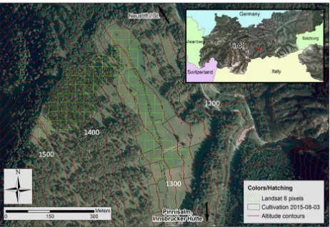
Figure 1: The Pinnis Valley test site (black polygon outlines).
of the unique cultivated grassland areas. On the last three field work days, measurements from the larch understory have been taken, too. The LS8 data contain therefore four scenes, which come from different acquisition paths and rows. The first three images are recorded from Worldwide Reference System (WRS)-2 path/row 193/(WRS)-27 with a viewing angle of (WRS)-2.9◦on the test site and the last one on October 12this from WRS-2 192/27 with a viewing angle of -6.4◦. Blue, green, red and Near-Infrared (NIR) bands were downloaded from the United States Geological Sur-vey (USGS) Earth Resources Observation and Science Center (EROS) Science Processing Architecture (ESPA) (United States Geological Survey, 2016) after processing to surface reflectance by using the LS8SR algorithm (United States Geological Survey, 2015b). Together with the surface reflectance bands, the NDVI was downloaded and the surface reflectance GI was calculated employing the ratio of surface reflectance green and red bands.
The collection of ground reference data involves the Cropscan MSR5, a field spectrometer mounted to a 3.5 m long pole with a footprint opening angle of 28◦. The field spectrometer band widths are actually designed to match the Landsat 4/5 Thematic Mapper (TM) instrument (Cropscan Inc., 2015). However, in the meantime band widths have not changed by more than 0.01µm, except for a massive band narrowing in the NIR channel of OLI. Table 1 compares the band widths for LS8 and field spectrometer.
Band Field spectrometer (µm) OLI (µm) OLI No.
Blue 0.45 - 0.52 0.45 - 0.51 2
Green 0.52 - 0.60 0.53 - 0.59 3
Red 0.63 - 0.69 0.64 - 0.67 4
NIR 0.76 - 0.90 0.85 - 0.88 5
Table 1: Comparison of field spectrometer and Operational Land Imager (OLI) bands.
The band narrowing in the LS8 NIR channel is due to the ex-clusion of an atmospheric water vapor extinction feature around 0.825µm. The comparison of surface reflectance data between Landsat 7 (LS7) and LS8 exhibits that the larger difference be-tween the NIR bands is “not evident” in surface reflectance data and the sensor-to-sensor difference is 1 % to 3 % on average (Flood, 2014). On all four days, 1399 measurements have been taken on the area, about 15 % thereof come from the larch un-derstory. Grassland areas have been sampled spatially regularly with the claim to obtain at least 30 measurements per area. Larch understory has been captured wherever possible as the field spec-trometer can - for technical reasons - take measurements only where irradiation is higher than 300 mW2 (Cropscan Inc., 2001).
This is achieved in sunlit patches in the forest.
3. METHODS
3.1 Sensor-to-Sensor Relationship
At first, an overlay of the satellite raster with the digitized culti-vation areas is performed. This results in 34 pixels on the larch forest area and 39 pixels on the cultivated grassland. The lat-ter number is slightly varying with time due to slightly changing cultivation polygon outlines. On the grassland, synthetic satellite pixels are generated from a linear weighted combination of the median values from all cultivation classes contributing to the area of the respective overlaying LS8 pixel. Each of the synthesized pixel values in each band is subtracted from the measured satellite value in the regarding pixel and the channel-wise mean is calcu-lated over all differences. The procedure is repeated for each of the field work days and the mean difference is called “bias” from now on.
3.2 Digital Forest
In order to reconstruct the larch forest with its geometrical prop-erties, a representative three-dimensional larch tree shapefile mod-eled in the way Bremer et al. (2013) describe is used. This shape-file is derived from a Light Detection and Ranging (LiDAR) scan of the forest acquired from the opposite slope in the year 2014. The shape was cut off a subset of about 35 tree shapes at the upper edge of the slope and transformed into a point cloud by sampling the three-dimensional shape with points in 2 cm dis-tance. The reason for this is that point clouds are computation-ally much easier to handle than shapefiles. Positions where to plant the virtual trees are determined using an inverse watershed algorithm tree delineation on a 1 m resolved normalized Digital Surface Model (nDSM) of the area. The procedure includes the application of a Gaussian Filter with search radius 2 m in order to smooth the nDSM and a reclassification to exclude vegetation lower than 5 m (similar approaches can be found in Eysn et al. (2015)). In this manner, 649 trees are identified on the slope and the chosen model tree is planted on each position using a 10 cm resolved Digital Terrain Model (DTM) as basis for planting. The tree point cloud is turned each time by some degrees such that the forest is not influenced by directional effects. Tree shadows in the forest are calculated using the Laserdata LIS (LIS) SADO (Sys-tem for the Analysis of Discrete Surfaces; B¨ohner et al. (1997); Rieg et al. (2014)) insolation multiscale module. For each of the LS8 overpass minutes, the direct mean insolation on a 1 cm re-sampled DTM is calculated and hard shadow areas are assigned where the result of this calculation is zero. The larch area frac-tion per LS8 pixel is determined by an overlay of the vertically projected digital larch trees with the pixel borders. However, as the single trees have lots of holes and single features and the pro-cedure has to be performed with vector data, the method becomes computationally very intensive. In order to keep it as easy as pos-sible, larch trees are for this analysis represented by circles each of which has exactly the same area as a vertically projected tree.
3.3 Larch Signal Extraction
The main method applied in this work is a linear spectral un-mixing based on an altered, extended and rearranged version of the unmixing equation presented in Roberts et al. (1998) (equa-tion 1).
ρtotal,λ,i= (AL,i·ρL,i,λ) + (AU,i·(ρfU,λ∗−b)) +ǫ (1)
at bandλ(unitless)
AL,i= larch area fraction of pixel i (unitless) ρL,i,λ= larch reflectance for pixel i (unitless) AU,i= understory area fraction for pixel i (unitless) ρfU,λ∗= understory reflectance measured with field
spectrometer at bandλ∗(unitless)
b= bias: field spectrometer minus satellite (unitless) ǫ= error term
The letterρ is used in general for reflectance values, but also counts for the vegetation indices NDVI and GI in this study, as they are also unmixed directly. The two biggest assumptions with this approach are the exclusion of non-linear processes, such as multiple scattering in the forest, and that the field spectrometer measurements mirror the natural variability of the class.ǫis gen-erally set to zero, consequently.
Equation 1 does not contain any shadow term and is therefore used to determine the larch reflectance with the “no shadows” method. For the shadow implementation, it has to be determined by which proportion the sunlit reflectance is reduced when shaded. The following values are introduced as Band Shadow Reduction Factors (BSRFs) and are estimated based on the work of Zhang et al. (2015) and Leblon et al. (1996).
• Blue: 0.1
• Green: 0.05
• Red: 0.1
• NIR: 0.2
They are applied to equation 2 in order to calculate the larch sig-nal when binary shadows are considered.
ρL,i,λ=
where As,i= shadow fraction per pixel (unitless) BSRFλ= BSRF for the respective band (unitless)
The terrain shadowing method includes both the hard larch tree shadows and an attempt to parametrize the shadows caused by the terrain, assuming that there is not a distinction between hard and no shadow only, but that there are continuous levels of shadow (equation 3).
where A˜s,i= shadow fraction for satellite pixel i (unitless)
n= number of DTM cells within a satellite pixel k, j= line, column coordinates of the shadow raster Ik,j= mean solar irradiance during one second at
the satellite overpass (W m2)
Imax, Imin= maximum and minimum ofIon the DTM area (W
m2)
The overall shadow fraction on a satellite pixel is calculated by an averaging of all hard shadows and all parametrized shadow values. The same equation 2 is used, butA˜s,iis inserted instead ofAs,i.
4. RESULTS
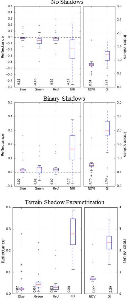
Table 2 informs about the mean differences between field spec-trometer synthesized pixels and original OLI reflectance values. All differences are below 0.6 %, with only some exceptions. The visible channels on July 15thexhibit differences up to 1.7 % and the NIR channel on July 15thand October 12thdiffers by 3.3 % and 5.6 % on average. Applying these results to the spectral un-mixing, the corrected OLI larch signal can be derived. Figure 2 shows the results for August 3rd, comparing the three shadow implementation methods. Boxes show the median values (red line), first and third quartile (boxes) and 1.5 times the interquartile range (whiskers). Every value beyond the latter range is marked as a cross and printed numbers are the median values.
For the “no shadows” method, all extracted larch surface reflec-tance median values are below zero. A large variability - as de-termined by the range covered by the whiskers - can be observed for the NIR band, even though in the negative range. Vegetation indices, however, are positive with a median value of 0.84 for the NDVI and 1.23 for the GI. Major changes arise when the bi-nary shadow method is employed. Surface reflectance becomes positive without exception and exhibits a 2 % reflectance in each visible band and 17 % in the NIR band. The variability in the NIR and green channel as well as in the NDVI is reduced to roughly the half of what is found when shadows are not considered. In contrast to that, the NDVI and GI median values show only rel-atively small changes. The NDVI is reduced to 0.75 and the GI increases to 1.99. Applying the terrain shadow method, changes observed are much smaller as compared to switching from no shadows to the binary shadow method. Variabilities are again re-duced, especially in the green and NIR band.
Figure 3 depicts the temporal evolution of the extracted median larch reflectances when derived with the three shadow methods presented. It can be clearly seen that the method without con-sidering shadows is not able to reproduce physically reasonable results as all found reflectances are negative. This is true for all dates. What cannot be revealed by the comparison of the boxplots in Figure 2 is that also the signal from the binary shadows method decreases with time (dashed lines). Especially October 12this a problematic case, where in fact the blue and green channels are still positive, while reflectance in the red range is equal to zero. The terrain shadow parametrization method, however, does not show this behavior. Values for the RGB range of the spectrum re-main constant or even show a slight increase over time, but do not become zero or negative. The NIR reflectance does not reduce as much as in the binary shadow case on October 12th, while the red reflectance even increases slightly.
Date (2015) SR B SR G SR R SR NIR
07-15 0.0122 0.0105 0.0165 -0.0333
08-03 0.0018 -0.0037 -0.0021 0.0014
09-01 0.0052 0.0029 0.0021 -0.0022
10-12 -0.0024 -0.0051 -0.0008 -0.0563
Figure 2: Comparison of the three shadow implementation meth-ods for the corrected larch signal on August 3rd, 2015.
As the terrain shadow parametrization method is the only method producing continuously physically reasonable results, Table 3 com-pares the found larch reflectance values with this method with values from two other studies.
Kajisa et al. (2007) investigated the spectral trajectory of a larch forest stand (Larix kaempferi, Japanese larch) in the experimen-tal forest of Kyushu University, Hokkaido, Japan, with increas-ing stand volume for Landsat 5 TM on Day of Year (DOY) 266. For this, they fitted an exponential decrease function to distinct data points which results in an asymptotic reflectance value for an increasing stand volume. The values found in this table are rounded numbers of the correlation coefficients as given in the
Figure 3: Temporal development of the extracted larch re-flectances without shadows considered, with binary shadows con-sidered and the terrain shadow parametrization applied. NoS stands for the no shadows-method, BS means binary shadows and TS is short for terrain shadows. The physically not reasonable range is shaded in yellow.
Band / Index
OLI (08-03)
OLI (09-01)
OLI (10-12)
Kobayashi et al. (2007) (ETM+)
Kajisa et al. (2007) (TM)
B 0.02 0.04 0.04 - 0.02
G 0.04 0.06 0.07 - 0.03
R 0.03 0.04 0.04 0.04 0.02
NIR 0.28 0.27 0.26 0.22 0.22
NDVI 0.72 0.59 0.57 0.69* 0.83*
GI 2.39 2.33 3.10 - 1.50*
Table 3: Comparison of the found values for the terrain shadow parametrization method on August 3rd (DOY 212), September 1st(DOY 244) and October 12th(DOY 285), 2015, with other studies. Compared is the median of the bias-corrected values for Landsat 8 Operational Land Imager (OLI) with the values found by Kobayashi et al. (2007) for Landsat 7 (LS7) Enhanced The-matic Mapper Plus (ETM+) andLarix gmeliniion DOY 170 and the values found by Kajisa et al. (2007) for Landsat 5 Thematic Mapper (TM) andLarix kaempferi on DOY 266. An asterisk means that the value was calculated from the found band spectral values in the study.
5. DISCUSSION
5.1 Field Spectrometer Measurements
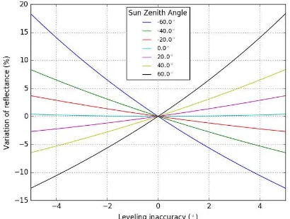
The field spectrometer values undergo a correction in two steps: first, radiation at the top of the sensor passes an ideal diffusely transmitting opal glass and is corrected for the sun zenith angle. The second correction includes the application of internal correc-tion factors for imperfect irradiance diffusion of the opal glass and small reflectance properties inside the module tube. These latter correction values come from a pre-delivery factory calibra-tion and should not be altered by the user (Cropscan Inc., 2001). In the former case, however, small inaccuracies in horizontal ad-justment of the radiometer can cause errors in reflectance mea-surement. As errors can reach high values, it is suggested not to use the field spectrometer when the sun zenith angle is bigger than 60◦(Cropscan Inc., 2001). This requirement has been ex-actly fulfilled as the maximum sun zenith angle for which mea-surements are taken is 59.2◦on October 12th. The lowest sun zenith angle is 25.8◦on July 15th
. Figure 4 shows how the mea-sured reflectance varies with different inaccuracies in the spec-trometer leveling at different sun zenith angles. Errors can reach
Figure 4: Sensitivity of the found reflectance to inaccuracies in leveling of the field spectrometer. Positive leveling inaccuracies mean a clockwise rotation of the field spectrometer when its front is positioned towards the sun, negative values indicate a counter-clockwise rotation.
up to an 18 % relative change of the reflectance measured for a sun zenith angle of∓60◦and a∓5◦horizontal adjustment er-ror. It can be seen that the errors are only relevant some values in the RGB range as their values mostly do not exceed 5.5 % and the error-relevant digits are therefore not considered in this study. However, as the NIR channel clearly exceeds 10 %, the errors be-come most relevant for this channel and increase over course of time. This could possibly explain the bigger difference between NIR values on October 12th, which reaches 5.6 %. Consider-ing all median NIR measurements for the respective cultivation areas, the±5 % error could explain a 6.2 % absolute error for reflectance measurements. It remains unsolved with this explana-tion why for example the reflectance difference on July 15thalso reaches 3.3 %. Besides the higher differences in the NIR band, the differences are in the range of or below the difference of 2 % that Flood (2014) found for a LS7 to LS8 surface reflectance sen-sor cross-calibration.
A means to improve the determination of sensor-to-sensor rela-tionship could be the introduction of Spectral Band Adjustment Factors (SBAFs) as described in Chander et al. (2013). They used
the ratio of sensor relative spectral responses in order to calculate SBAFs, which relate the reflectance measurements of one sensor with those of another one on pseudoinvariant test sites. However, the approach cannot be put into practice in this study as the exact relative spectral response is not known for the field spectrometer.
5.2 Viewing Geometry
On a more general level, it has to be accounted for the fact that the cultivation area itself belongs to a slope and is not perfectly suited for a sensor-to-sensor calibration. Other studies suggest to use deserts or at least flat and homogeneous areas (confer e.g. Czapla-Myers et al., 2015; Mishra et al., 2014). The slope has been used nevertheless, because it is very close to the larch for-est and other sites suited for calibration are not reachable within some kilometers distance. This is a logistic problem as mea-surements have to be temporally close to satellite overpasses. In this context it has to be addressed, too, that field spectrometer and satellite do not have the same viewing geometry. The LS8 images claim to be taken in “nadir” view (as adopted from the image metadata), the Pinnis test site is 2.4◦for WRS-2 193/27 and -6.9◦for WRS-2 192/27 away from the absolute nadir view though. Figure 5 gives an impression of the two satellite views on the test site. Apart from the fact that the viewing direction is
Figure 5: The Pinnis test site is located opportune on the over-lapping area of two descending Worldwide Reference System (WRS)-2 paths, shown in blue. As can be identified from the centerlines of the images acquired in row 27, the center of path 193 is closer to the test site than that of path 192. Also the view direction switches between the two acquisition positions.
also random, but the terrain is inclined. The effects of this com-bination should actually be included in the LS8 preprocessing. As topography varies also on much smaller scales than the 30 m resolution of the correction Digital Elevation Model (DEM) used in the processing (United States Geological Survey, 2015a), the effects of small-scale slope variation are still to be investigated.
5.3 Larch Signal Extraction
Comparison of the found larch reflectance with the terrain shadow parametrization method with the two studies Kobayashi et al. (2007) and Nakaji et al. (2008) shows that values are equal in range, even though many deviations exceed 10 % relative change. Differences can be explained by the use of different sensor (ETM+ and TM), different measurement dates, different larch species and different climatic conditions.
Concerning the performance of the applied shadow methods, an assessment which of the three shadow methods is the most ac-curate one is only possible on the basis of comparison to the two studies mentioned above and the temporal evolution of larch reflectance medians extracted with the three shadow methods. What can be proven is that shadows have to be considered, when the larch tree surface reflectance shall be derived. The reason is that all extracted band reflectances without considering shad-ows are negative. This is physically not meaningful and, conse-quently, the method is not applicable for deriving band reflectance. By contrast, the comparison of the binary and the terrain shadow parametrization method demands a closer examination. Only the zero red reflectance on October 12thgives a hint on the reliabil-ity of the binary shadow method, because all other values seem to agree well with the findings by Kobayashi et al. (2007) and Nakaji et al. (2008). Assuming that also this method could be marked up as a big step towards the “truth”, but not the most accurate one, the terrain shadow method is the most plausible ap-proximation to the true and overall larch signal. Due to the fact, however, that BSRFs have been read from diagram values and depend in reality on the object characteristics considered (grass, soils...), it is obvious that also the terrain shadow parametrization method is a limited approach. Moreover, the terrain shadow is just parametrized and based on a bilinear interpolation of a 1 m resolved DTM, which is also just a model approach. Generally, the method of spectral unmixing might be easier applicable to spruce trees or other “dense” trees, as they grow in more regular shapes, have a relatively higher Leaf Area Index (LAI) and allow less sunlight to penetrate the crown (Lio, 2014). Nevertheless, it could be shown that even for a complex-structured larch forest the unmixing delivers solid results. The vegetation indices NDVI and GI found to be in the range of values found by Kajisa et al. (2007) even without considering shadows at all. This could be a hint that these vegetation indices are relatively unaffected by shadow, as shown for the NDVI and GI in Zhang et al. (2015).
If not only the median of the found larch reflectance is consid-ered, the inter-pixel variability is still very high, especially in the important NIR band. Still, absolute NIR reflectance variability is generally higher as could be observed for the field spectrome-ter measurements on the grassland area. This variability for trees might come on the one hand from the natural reflectance vari-ability of the real trees as captured on the LS8 image. On the other hand it can also be a result of different phenological states of the single trees and mutual shadowing. As the overall tree sig-nal as a combination of sunlit and shadowed parts is captured, also mutual shadowing of crowns becomes an important factor (Li and Strahler, 1992). The found results are not suitable for an exact species identification as there are simply too few channels
involved. Nevertheless, they can definitely be used for classi-fication purposes. For example, they could serve as class cen-ters and variability estimates for a supervised classification. The classification accuracy, for example compared to a manual train-ing, should be explored in further analyses. However, coming closer to a species-specific spectral signature, the inclusion of more spectral bands and more viewing directions would be ne-cessary.
Concerning the geometrical approach with 3D tree shapes applied here, the main advantages of this method are the simplicity and computational effectiveness. As mentioned in section 1, Li and Strahler (1985) used an even simpler approach with cones rep-resenting conifers casting shadow on a contrasting background. The fact that all of the attributes they found important - shape, form and shadowing - are considered also in this study reflects the feasibility of the method. Of course, the larch tree fraction calculation with the help of circles representing the single trees is a heavy assumption. Especially at pixel borders inaccuracies can happen as the circle diameter is not as large as the tree diameter. However, as the effect occurs from both sides, it evens out.
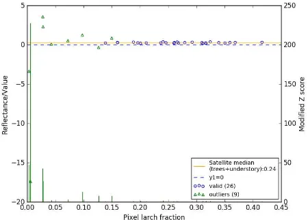
By the example of the NIR channel on August 3rd, Figure 6 re-veals that there are many outliers found in the larch spectral un-mixing procedure. They are illustrated by displaying the
modi-Figure 6: Many larch Near-Infrared (NIR) outliers are found when the pixel larch fraction is smaller than 0.1.
One general issue in this study is, however, that the results cannot be proven and there is - despite comparisons - no reference and “truth” value given. Chosen BSRFs are just estimates and there-fore arbitrary. Even though the found reflectances are roughly coherent with findings of related work, a simulation of differ-ent BSRF combinations is desirable. Another approach could be measuring with a field spectrometer which is also able to deal with shadow reflectances.
6. CONCLUSIONS AND OUTLOOK
This work investigates the spectral signal of a larch forest stand (Larix deciduaMILL.) in Pinnis Valley (Tyrol, Austria). The main goal is to extract the larch tree spectral signal in Landsat 8 (LS8) Operational Land Imager (OLI) visible and Near-Infrared (NIR) surface reflectance channels, using combined ground- and satellite-based measurements. The described procedures for a-chieving this goal are computationally inexpensive and based on a linear spectral unmixing approach. The ground data include measurements of the larch forest understory with the Cropscan Multispectral Radiometer with five bands (MSR5) with OLI-like channels, simultaneously to satellite overpasses on August 3rd, September 1stand October 12th, 2015. In order to account for sensor-to-sensor differences, the relationship between ground- and satellite measurements is investigated on these three days, and July 15th, additionally: field spectrometer values have been taken for each of the cultivated parcels and based on a spatial overlay, LS8 pixels are generated synthetically from these measurements. The mean difference between field spectrometer and satellite for the respective bands is used to correct the field spectrometer val-ues for the mean ground-to-satellite difference in the unmixing procedure. All found differences in the visible range of the spec-trum are small as compared to sensor-to-sensor differences that other studies found (cf. e.g. Flood, 2014), except for the visible channels on July 15thand NIR values on July 15thand October 12th. Some of these inaccuracies can be explained by errors in spectrometer horizontal alignment at high sun zenith angles.
For the larch signal extraction procedure a digital forest has been built, consisting of 649 three-dimensional modeled trees extracted from a 1 m resolved normalized Digital Surface Model (nDSM) of the area, employing an inverse watershed tree delineation algo-rithm. The tree area per Landsat pixel is derived from the area of perpendicularly projected circular model trees. A comprehensive shadow modeling has been performed by testing three shadow methods. Hard shadows were calculated from tree point clouds in 2 cm resolution for each of the satellite overpasses and ground shadow rasters were derived from that. The larch signal was de-rived for three cases: no shadows considered, only hard shad-ows from the trees (binary shadshad-ows) and a combination of hard shadows and a terrain shadowing parametrization. Without con-sidering shadows, the only usable signals have been found the Normalized Difference Vegetation Index (NDVI) and Greenness Index (GI) with values at least in the order of magnitude the found indices by Kajisa et al. (2007) including shadows. This could indicate that, indeed, these indices are quite “shadow-resistant”, even though this hypothesis has to undergo further testing. The surface reflectance channels show negative values without excep-tion. For the binary shadow method, a big step forward could be made: all reflectances found with this approach are positive and in a physical meaningful range, except for the red band on Octo-ber 12th, 2015, which is zero. A further improvement is reached with parametrizing the terrain shadowing by an inversion of the radiation amount that is received during the satellite overpasses. The found larch signals with this method are positive without ex-ception and agree well with the findings from other studies (cf.
Kobayashi et al., 2007; Kajisa et al., 2007). Uncertainties of the procedure remain principally in the inexact tree shape represen-tation, missing comprehensive and distributed measurements of the underground and estimated parameters for a reduction from sunlit to shadow reflectance.
In future studies, the workflow presented can be further devel-oped. Even though it will be computationally much more expen-sive, latest advances in technology use laser scanners mounted on Unmanned Aerial Vehicles (UAVs) (cf. e.g. Wallace et al., 2012). With this method it is possible to scan the whole forest in much higher precision and within shorter time. Laser scanning the forest from above and not from the opposite slope allows further to model tree shapes much more exact without missing backsides. Every tree’s own shape is depicted and hence a fully determined geometrical view of the forest with better estimates of larch area per pixel and shadow fractions can be established. This geometrical view can then also include sensor and sun ge-ometry which enables a better quantitative estimation of the influ-ences that for example a change in acquisition path has. Mount-ing a field spectrometer on a UAV would further allow to capture the forest and underground signal spatially referenced at a higher resolution. Reflectance values could be captured within a much shorter range of time around the satellite overpass, coming closer to the real viewing and sun. In order to compare results and sup-ply real ”truth” data, a radiative transfer modeling of the forest could be performed in order to compare the two datasets (cost-effective method presented here and intensive radiative transfer modeling).
With respect to the satellite resolution, big steps towards better re-sults can be made with the Sentinel 2A (SEN-2A) satellite. Com-pared to LS8, its ground sampling distance is 10 m and therefore three times higher. Furthermore, at the latitude of the Pinnis test site the revisiting time will be reduced to two or three days to-gether with Sentinel-2B whose launch is planned for mid of 2016 (European Space Agency, 2016).
Summing up, this work contributes to the field of ground truth data collection and comparison in remote sensing as it supplies a comparison of computationally inexpensive approaches to ex-tract the larch tree spectral signal. Ground to satellite sensor differences are found small in general, nevertheless field spec-trometer values have been adjusted to fit the satellite values. The method that accounts for both the larch hard shadows and a ter-rain shadow parametrization is found most accurate for the signal extraction. However, future work has to be done in order to in-vestigate error sources quantitatively and set up a database for comparison.
ACKNOWLEDGEMENTS
We would like to thank all field work volunteers for the great support: Carina Draschl, Robert Niederheiser and Cindy Rabe. Further, we would like to thank Frederic Petrini-Monteferri from Laserdata GmbH, Innsbruck, for supplying the insolation mod-ule.
References
B¨ohner, J., K¨othe, R. and Trachinow, C., 1997. Weiterentwick-lung der automatischen Reliefanalyse auf der Basis von dig-italen Gel¨andemodellen. G¨ottinger Geographische Arbeiten 100, pp. 3–21.
cloud data of varying quality.{ISPRS}Journal of Photogram-metry and Remote Sensing80, pp. 39 – 50.
Chander, G., Mishra, N., Helder, D., Aaron, D. B., Angal, A., Choi, T., Xiong, X. and Doelling, D. R., 2013. Applications of spectral band adjustment factors (SBAF) for cross-calibration. Geoscience and Remote Sensing, IEEE Transactions on51(3), pp. 1267–1281.
Colwell, J. E., 1974. Vegetation canopy reflectance.Remote Sens-ing of Environment3(3), pp. 175–183.
Cropscan Inc., 2001. Multispectral Radiometer User’s Manual. Cropscan Inc. No explicit author given.
Cropscan Inc., 2015. Cropscan Inc. Web Page. http:// cropscan.com/msr.html. Accessed: 2015-10-04.
Czapla-Myers, J., McCorkel, J., Anderson, N., Thome, K., Big-gar, S., Helder, D., Aaron, D., Leigh, L. and Mishra, N., 2015. The ground-based absolute radiometric calibration of Landsat 8 OLI.Remote Sensing7(1), pp. 600–626.
European Space Agency, 2016. Sentinel-2b new launch date announced. http://www.esa.int/Our_Activities/ Observing_the_Earth/Copernicus/Sentinel-2/New_ launch_date_set_for_Sentinel-2A. Accessed: 2016-04-04.
Eysn, L., Hollaus, M., Lindberg, E., Berger, F., Monnet, J.-M., Dalponte, M., Kobal, M., Pellegrini, M., Lingua, E., Mongus, D. et al., 2015. A benchmark of LiDAR-based single tree detection methods using heterogeneous forest data from the Alpine space.Forests6(5), pp. 1721–1747.
Flood, N., 2014. Continuity of reflectance data between Landsat-7 ETM+ and Landsat-8 OLI, for both Top-of-Atmosphere and surface reflectance: A study in the Australian landscape. Re-mote Sensing6(9), pp. 7952–7970.
Gao, F., He, T., Masek, J. G., Shuai, Y., Schaaf, C. B. and Wang, Z., 2014. Angular effects and correction for medium resolu-tion sensors to support crop monitoring. Selected Topics in Applied Earth Observations and Remote Sensing, IEEE Jour-nal of7(11), pp. 4480–4489.
Holben, B. and Fraser, R. S., 1984. Red and near-infrared sensor response to off-nadir viewing.International Journal of Remote Sensing5(1), pp. 145–160.
Iglewicz, B. and Hoaglin, D. C., 1993. How to detect and handle outliers. Vol. 16, Asq Press.
Kajisa, T., Murakami, T., Mizoue, N. and Yoshida, S., 2007. Dif-ferences in spectral trajectory with stand volume development between Japanese larch and Japanese oak in Hokkaido, Japan. Journal of forest research12(6), pp. 435–441.
Kobayashi, H., Suzuki, R. and Kobayashi, S., 2007. Reflectance seasonality and its relation to the canopy leaf area index in an eastern Siberian larch forest: Multi-satellite data and radia-tive transfer analyses.Remote Sensing of Environment106(2), pp. 238–252.
Koch, B., Ammer, U., Schneider, T. and Wittmeier, H., 1990. Spectroradiometer measurements in the laboratory and in the field to analyse the influence of different damage symptoms on the reflection spectra of forest trees. International Journal of Remote Sensing11(7), pp. 1145–1163.
Leblon, B., Gallant, L. and Granberg, H., 1996. Effects of shadowing types on ground-measured visible and near-infrared shadow reflectances. Remote Sensing of Environment58(3), pp. 322 – 328.
Li, X. and Strahler, A. H., 1985. Geometric-optical modeling of a conifer forest canopy. Geoscience and Remote Sensing, IEEE Transactions on(5), pp. 705–721.
Li, X. and Strahler, A. H., 1992. Geometric-optical bidirectional reflectance modeling of the discrete crown vegetation canopy: Effect of crown shape and mutual shadowing.Geoscience and Remote Sensing, IEEE Transactions on30(2), pp. 276–292.
Lio, A.; Ito, A., 2014. A Global Database of Field-observed Leaf Area Index in Woody Plant Species, 1932-2011.
Mishra, N., Haque, M. O., Leigh, L., Aaron, D., Helder, D. and Markham, B., 2014. Radiometric Cross Calibration of Landsat 8 Operational Land Imager (OLI) and Landsat 7 En-hanced Thematic Mapper Plus (ETM+). Remote Sensing 6(12), pp. 12619–12638.
Nakaji, T., Ide, R., Takagi, K., Kosugi, Y., Ohkubo, S., Nasahara, K. N., Saigusa, N. and Oguma, H., 2008. Utility of spectral vegetation indices for estimation of light conversion efficiency in coniferous forests in Japan. agricultural and forest meteo-rology148(5), pp. 776–787.
Rieg, L., Wichmann, V., Rutzinger, M., Sailer, R., Geist, T. and St¨otter, J., 2014. Data infrastructure for multitemporal airborne lidar point cloud analysis–examples from physical geography in high mountain environments.Computers, Environment and Urban Systems45, pp. 137–146.
Roberts, D. A., Gardner, M., Church, R., Ustin, S., Scheer, G. and Green, R., 1998. Mapping chaparral in the santa monica mountains using multiple endmember spectral mixture models. Remote Sensing of Environment65(3), pp. 267–279.
Rouse, J., Haas, R., Schell, J., Deering, D. and Harlan, J., 1974. Monitoring the vernal advancements and retrogradation of nat-ural vegetation. NASA/GSFC, Final Report, Greenbelt, MD, USApp. 1–137.
Suits, G. H., 1973. The cause of azimuthal variations in direc-tional reflectance of vegetative canopies. Remote Sensing of Environment2, pp. 175–182.
Sukuvaara, T., Pulliainen, J., Kyr¨o, E., Suokanerva, H., Heikki-nen, P. and SuomalaiHeikki-nen, J., 2007. Reflectance spectrora-diometer measurement system in 30 meter mast for validat-ing satellite images. In: Geoscience and Remote Sensing Symposium, 2007. IGARSS 2007. IEEE International, IEEE, pp. 2885–2889.
United States Geological Survey, 2015a. Landsat 8 (L8) Data Users Handbook. United States Geological Survey.
United States Geological Survey, 2015b. Provisional Landsat 8 Surface Reflectance Product Guide.
United States Geological Survey, 2016. United States Geologi-cal Survey Earth Resources and Observation Science (EROS) Center Science Processing Architecture.https://espa.cr. usgs.gov/login/?next=/. Accessed: 2016-04-10.
Wallace, L., Lucieer, A., Watson, C. and Turner, D., 2012. De-velopment of a uav-lidar system with application to forest in-ventory.Remote Sensing4(6), pp. 1519–1543.
Zarco-Tejada, P. J., Berj´on, A., L´opez-Lozano, R., Miller, J., Mart´ın, P., Cachorro, V., Gonz´alez, M. and De Frutos, A., 2005. Assessing vineyard condition with hyperspectral in-dices: Leaf and canopy reflectance simulation in a row-structured discontinuous canopy. Remote Sensing of Environ-ment99(3), pp. 271–287.