(Why) Should We Use SEM?
Pros and Cons of Structural Equation Modeling
Christof Nachtigall1,2, Ulf Kroehne, Friedrich Funke, Rolf Steyer
Friedrich Schiller University of Jena
During the last two decades, Structural Equation Modeling (SEM) has evolved from a statistical technique for insiders to an established valuable tool for a broad scientific public. This class of analyses has much to offer, but at what price? This paper pro-vides an overview on SEM, its underlying ideas, potential applications and current software. Furthermore, it discusses avoidable pitfalls as well as built-in drawbacks in order to lend support to researchers in deciding whether or not SEM should be inte-grated into their research tools. Commented findings of an internet survey give a “State of the Union Address” on SEM users and usage. Which kinds of models are preferred? Which software is favoured in current psychological research? In order to assist the reader on his first steps, a SEM first-aid kit is included. Typical problems and possible solutions are addressed, helping the reader to get the support he needs. Hence, the paper may assist the novice on the first steps and self-critically reminds the advanced reader of the limitations of Structural Equation Modeling
Keywords: Structural equation modeling (SEM), internet survey, SEM software, AMOS, EQS, LISREL
1
Correspondence concerning this article should be addressed to Christof Nachtigall, Friedrich Schiller Universität Jena, Institute for Psychology, Steiger 3 Haus 1, 07743 Jena, Germany, E-mail: [email protected]
2
(Why) should we use SEM?
“The techniques of Structural Equation Modeling represent the future of data analysis.” “Nobody really understands SEM.”
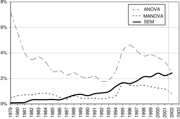
These quotes from our internet survey mark the divergent points of view. More than other statistical tools, SEM inspires enthusiastic praise as well as persistent rejection. On the one hand, SEM allows for conducting and combining a vast variety of statistical procedures like multiple regression, factor analysis, (M)ANOVA and many others. But, on the other hand, SEM is often seen as complicated and difficult to understand. The requirements in sample size appear vague and the interpretation of the results should be labeled “handle with care”. Nevertheless, SEM is getting more and more popular. As can be seen in Figure 1, the citation frequency in psychological literature has steadily increased since the late seventies, meanwhile reaching the popularity of ANOVA.
0% 2% 4% 6% 8%
1979 1980 1981 1982 1983 1984 1985 1986 1987 1988 1989 1990 1991 1992 1993 1994 1995 1996 1997 1998 1999 2000 2001 2002 2003
ANOVA MANOVA SEM
Figure 1: Citation frequencies of SEM and (M)ANOVA in the APA PsycINFO -
data-base3 between 1979 and 12/2002. The numbers are standardized with respect to the
to-tal number of records per year.
How can researchers decide whether to use SEM or not? This paper presents advan-tages and pitfalls of this technique in order to help potential users in deciding whether
3
its application is of interest. An overview of the basic ideas, possibilities and prerequi-sites of SEM will be provided for the novice SEM user. Readers already familiar with SEM will find information on facilitated usage, as well as some critical remarks on pos-sible drawbacks and traps.
This paper is written with the background of several years of SEM consulting given by the authors. It represents a compilation of our experience in discussing SEM applica-tions with other colleagues and students. This paper presents a personal view, although it is supplemented by data of an internet questionnaire on current knowledge, attitudes and application of SEM in the field of psychology.
The paper is divided into three sections: An initial summary on the principles of SEM (which may be skipped by readers who are already familiar with this topic) is followed by the results of the survey. The third section discusses some prominent pros and cons concerning the application of SEM. Finally, some helpful information resources on cur-rent SEM network and its features have been added at the end of the paper.
A short description of SEM
In introductory SEM books (e.g. Hoyle, 1995; Kline, 1998; Maruyama, 1998; or Raykov & Marcoulides, 2000), a simple and accurate definition of SEM is hard to find. Kaplan (2000, p. 1) proposes, that “structural equation modeling can perhaps best be defined as a class of methodologies that seeks to represent hypotheses about the means, variances and covariances of observed data in terms of a smaller number of ‘structural’ parameters defined by a hypothesized underlying model”. What exactly does this mean? Beside the problem, that the terms ‘structural’ and ‘model’ themselves need clarifica-tion, the definition points out central features: SEM represents a multitude of tech-niques ‘under one umbrella’, which might be explained more comprehensibly by its core concepts and typical examples.
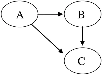
variable C, and A also having an effect on C4. In contrast to ordinary regression
analy-sis SEM considers several equations simultaneously. The same variable may represent a predictor (regressor) in one equation and a criterion (regressand) in another equation. Such a system of equations is called a model. Hoyle (1995) points out, that the term
model might be unfamiliar to some readers, but the concept itself probably is not. “At the most basic level, a model is a statistical statement about the relations among vari-ables” (p. 2). In the model depicted in Figure 2, the total effect of A on C can be de-composed into the direct effect of A on C and the indirect effect mediated via B.
Figure 2: A model of the regressive dependencies between three variables, written as
a path diagram. The path diagram represents a simple linear regression of B on A and a multiple linear regression of C on B and A.
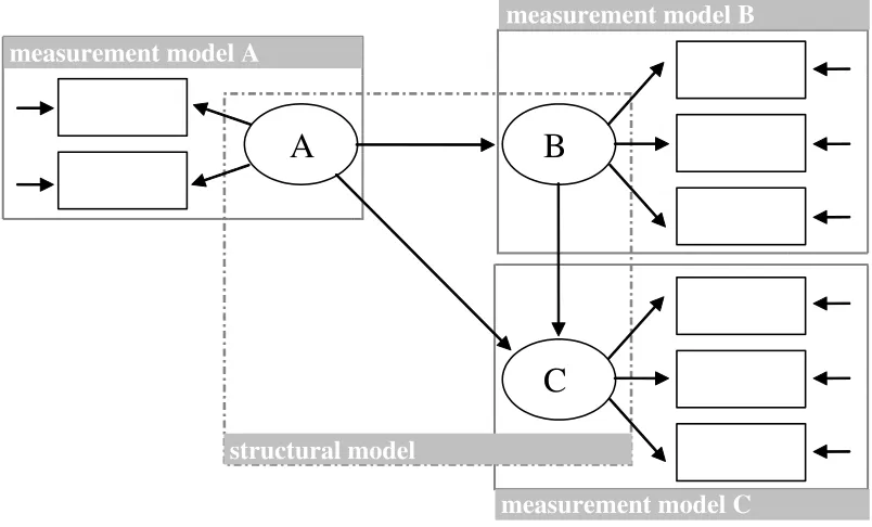
Path diagrams and the calculation of direct, indirect and total effects stem from the methodology of path analysis, developed by the biometrician Sewall Wright (1921, 1934) more than 70 years ago. SEM includes this technique but offers much more. Its most prominent feature is the capability to deal with latent variables, i.e. nonobservable quantities like true-score variables or factors underlying observed variables. Latent vari-ables are connected to observable varivari-ables by a measurement model (see Edwards and Bagozzi (2000) for an extensive discussion of the mathematical and epistemological na-ture of those relations). Structural Equation Models, therefore, consist of a structural model representing the relationship between the latent variables of interest, and meas-urement models representing the relationship between the latent variables and their manifest or observable indicators (Figure 3).
4 Mathematically, these effects are ordinary (if there is only one predictor) or partial regression
coeffi-cients (if there are two or more predictors).
A B
Figure 3: An expanded model of the regressive dependencies between three latent vari-ables illustrating the distinction between the structural model and the measurement models.
What does SEM do?
Its main feature is to compare the model to empirical data5. This comparison leads to
so-called fit-statistics assessing the matching of model and data. If the fit is acceptable, the assumed relationships between latent and observed variables (measurement models) as well as the assumed dependencies between the various latent variables (structural model) are regarded as being supported by the data. Strictly speaking, the assumed model is not rejected. In some cases, only the fit of a measurement model is of interest (for instance variable C and its indicators in Figure 3). In this case, a SEM is a confir-matory factor analysis model (CFA). In other cases, the parameters of the structural model may be of interest. For example, the regression coefficients characterizing the arrows in Figure 3 are generally not predetermined by the user but estimated and tested with a SEM program. The substantive question may be, if A has a direct effect on C, or if there is an indirect effect via B (i.e. if B is a mediator, see Baron and Kenny, 1986 for a distinction of mediators and moderators).
5 More specifically, the model implies a specific structure of the (means and) covariances which can be
compared to the (means and) covariances in the sample.
A B
C
measurement model A
measurement model C measurement model B
What SEM does not do
Even though we used the term effect, this does not mean that a Structural Equation Model is a causal model. This misinterpretation of SEM remains to be eradicated in popular introductory textbooks (e.g. Backhaus et al., 2000). Although under specific circumstances, SEM can represent causal relationships, a well-fitting SEM does not nec-essarily have to contain any information on causal dependencies at all. Arrows may be drawn one way or the other way around, leaving the fit of a model unaffected (for more details on this topic compare Raykov & Penev, 2001; or Stelzl, 1983). Hence, testing the fit of a SEM is not a test of causality. However, many SEM users are at least implicitly interested in causal modeling. The work of Bollen (1989, chap. 3), Nachtigall, Steyer and Wüthrich-Martone (2001) or Steyer (2003, chap. 15-17) provides an introduction to this topic. Influential approaches on causation and causal effects have been elaborated and propagated by Rubin (1974, 1986, see also Holland & Rubin, 1988; Rosenbaum & Rubin; 1983), Pearl (2000), and Spirtes, Glymour & Scheines (1993). A mathematically formalized theory of causal regression models has been developed by Steyer (Steyer, 1992, 2003; Steyer, Gabler, von Davier, Nachtigall, & Buhl, 2000a; Steyer, Gabler, von Davier, & Nachtigall, 2000b; Steyer, Nachtigall, Wüthrich-Martone, & Kraus, 2002). Within this framework, strategies for testing causal dependencies in SEM have been introduced (Steyer, 1988, chap. 23; von Davier, 2001), although these tests are not available in commercial SEM programs.
SEM in practice
Since the initial publications of Karl Jöreskog on confirmatory factor analysis and LISREL (Jöreskog, 1967, 1969, 1973, 1978), the application of SEM was solely reserved to specialists who were experienced with matrix algebra and able to handle the compli-cated program code of the former SEM software. Today, programs like AMOS 5, LISREL 8.5 or EQS 5.7 provide a graphical user-interface allowing the user to configure path diagrams, calculate model fit, and estimate parameters with a few mouse clicks. Thus, the demands on the user to ‘run’ a model have dramatically decreased, permitting SEM software application without much statistical knowledge.
Which type of data does SEM need?
esti-mation of means and intercepts of latent variables. Most contemporary SEM software versions can handle (even incomplete) raw data input files (AMOS 5, LISREL 8.5 with PRELIS, EQS 5.7, Mplus 2.12), making the application even more comfortable.
To apply SEM, an adequate sample size is required and the data usually have to meet distributional assumptions. Current SEM software has different procedures at hand. The most common type of estimating parameters and computing model fit is the Maximum Likelihood Method (ML) requiring multivariate normally distributed con-tinuous variables. The sample size, as a rule of thumb, is recommended to be more than 25 times the number of parameters to be estimated, the minimum being a subject-parameter-ratio of 10:1. The lower bound of total sample size should be at least 200 (Kline, 1998). The method of Weighted Least Squares (WLS) offers an alternative, as-ymptotically distribution-free (ADF) approach, but the sample size must be exception-ally large, which is often not available in psychological research (Muthén & Kaplan, 1985, 1992). Simulation studies by Yung and Bentler (1994) propose a minimum sample size of 2000 to obtain satisfactory results. In general, the accuracy and stability of SEM results declines with decreasing sample size as well as with increasing number of vari-ables. Hoyle (1999) provides advice concerning this topic. The WLS method also pro-vides an attractive approach to the analysis of variables which are ‘only’ ordinal (Jöre-skog, 2001).
Because of the interdependence of the model to be analyzed and the accuracy of pa-rameter estimation and statistical inference, bootstrap algorithms are recommended as the upcoming procedure (Bollen & Stine, 1993; Yung & Bentler, 1994). Bootstrapping is a technique of drawing many pseudoreplicate samples out of a given dataset. This re-sampling may help to calculate standard errors even if distributional assumptions are violated (Efron & Tibshirani, 1985).
An Internet Survey
Sample: The effective sample consisted of N = 87 responders. 53 subjects were
ex-perienced with SEM. Subjects categorized themselves into four groups of psychological researchers as shown in Table 1.
Table 1
Frequency Table of Self-Categorized Groups (Type of Researcher)
The academic members of the sample can be divided into graduate students (59%), Ph.D.s (28%) and subjects with higher qualifications (13%).
Results: 60% of subjects expected SEM to be used more frequently in the future,
11.5% expected an even stronger increase, while only 2.2% believed that SEM usage will decrease. From those who have SEM experience (N=53), 37.8% called it an outstanding statistical tool. Hence, the desirability of an increased usage, measured on a seven point rating scale was judged positively with a mean value of +1.06 (SD=1.2, N=87, p<.05, the neutral point of the scale was 0). The different groups (substantive researchers, method researchers and students) do not differ in their judgment. As an interesting finding, the estimated importance of SEM, as well as the estimated desirability of an increased usage do not correlate with subjects' self-rated knowledge or with practical experience.
Why should we use SEM? The possibility of modeling complex dependencies (95%) and latent variables (82 %) were regarded as being the main advantages, as well as the main reasons to use SEM. Guidelines by supervisors (13%) or an expected pushing of the publication probability (6%) were not that important. Disadvantages of SEM have been assessed with an open ended question, providing a wide range of heterogeneous problems like the complexity of theory and application, the danger of producing models post hoc, neglecting substantive background, high data requirements and others. Sub-jects had the opportunity to formulate their wishes in order to better understand SEM. Table 2 shows that especially a need for comprehensive textbooks exists.
Substantive researchers
Methodological researchers
Practitioners Students
46 13 2 26 Absolute
53 15 2 30 Percent
Table 2
Frequency Table (Percentage) of the Item: “What doYou Wish Concerning SEM?”
All Subgroups
Substantive
researchers
Methodological
researchers Students
More comprehensible textbooks 63 61 46 73
More textbooks at all 14 9 23 19
More workshops on SEM 30 24 46 31
More lectures / courses 47 39 61 54
More multimedia material 25 22 31 27
Note. (multiple choice possible, N = 87)
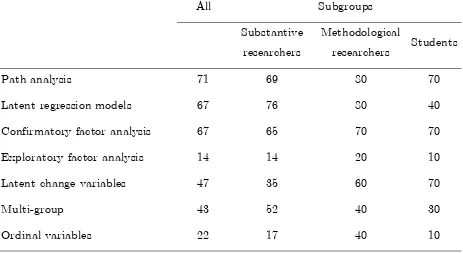
What kinds of SEM models are most frequently used and which software is applied for this purpose? Table 3 shows the frequencies of different types of models.
Table 3
Frequency Table (Percentage) of the Item: “Which Type of Models do You Use for Your
SEM Analysis?”
All Subgroups
Substantive researchers
Methodological
researchers Students
Path analysis 71 69 80 70
Latent regression models 67 76 80 40
Confirmatory factor analysis 67 65 70 70
Exploratory factor analysis 14 14 20 10
Latent change variables 47 35 60 70
Multi-group 43 52 40 30
Ordinal variables 22 17 40 10
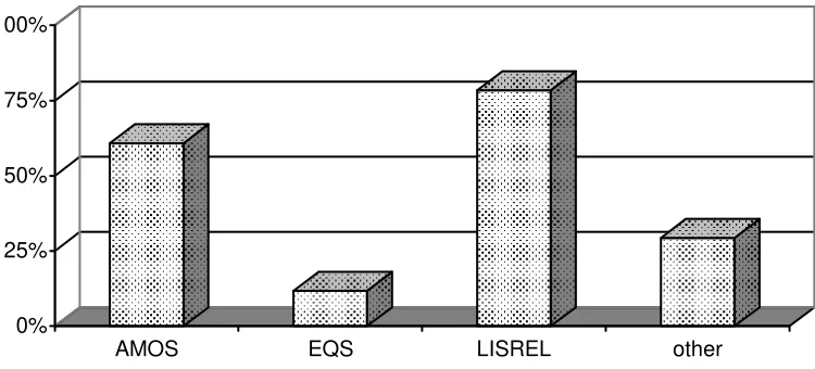
The results were in accordance with the judgments of the main reasons to use SEM and with its main advantages. Concerning the software used by the subjects, Figure 4 presents the frequencies of the different SEM packages (N=53).
0% 25% 50% 75% 100%
AMOS EQS LISREL other
Figure 4. Frequencies of the kind of software used by the subjects (N=53).
Comment: AMOS (Version 4); LISREL (both Syntax and SIMPLIS); other (MX, SAS, STREAMS, Mplus).
Pros and Cons of SEM
inter-pretation of latent variables, since substantive researchers may be more familiar with the true scores underlying well known scales than with latent variables based on com-plex and perhaps not theory-based measurement models. Finally, as the effect size and not the significance of parameters is of interest (remember that SEM needs a consider-able sample size), the use of manifest instead of latent variconsider-ables could be compensated by taking lower bounds for the interpretation of parameters.
However, latent variable modeling, if conducted skillfully, offers more than mere re-moving of measurement errors. In appropriate repeated measurement designs, not only a decomposition of observed variables (strictly speaking: their variances and covariances) into true scores and errors is feasible, but the true-score variables, containing situational factors, can be further decomposed into so-called trait variables and corresponding re-siduals (Latent State Trait Models, e.g. Steyer, Ferring & Schmidt, 1992). Not only per-sonality psychologists will find plenty of potential theoretical applications for such mod-els.
SEM is designed for the analysis of the relationships between latent variables. How-ever, diagnostic researchers wish to know the values of latent variables (i.e. the factor scores) for individual subjects. They can be estimated in SEM. However, these estima-tions (like all the other estimation methods available yet) bear severe problems, as fac-tor scores may be derived in different ways and are ambiguous. Bollen (1989, pp. 305-306) warns, that researchers “should refrain from too fine comparisons of standings on factor scores, for they may be asking more from the factor score estimates than they can provide” (compare also Jöreskog, 2001; Raykov & Penev, 2001, 2002).
data (Jöreskog, Sörbom, du Toit and du Toit (1999) for ordinal variables respectively Muthén, 2001a; Muthén, 2001b for categorical variables).
So what? Luxury we can afford? So much light without shade? Our experience in SEM-consulting gives the following impression: Some of the features of SEM allow re-searchers to travel on the Via Regia of quantitative methodology, since most editorial boards seem to rank SEM very high. At the same time, the method tempts us to leave the King’s Road and deter in dead ends. Some of the dead ends could be avoided by skilful drivers with precise road maps. Others are not immediately recognizable as being rough roads, as they are inevitable. We just have to accept that even with a sound un-derstanding we reach the limits of the methods and encounter built-in problems of SEM. Summing up the substance of the metaphor we have to conclude that some of the common mistakes are avoidable with a sound understanding of what we are doing, oth-ers are not.
The causes of some common mistakes can be explained from the perspective of soci-ology and history of science. SEM owes its popularity to the illustrative power of path diagrams. This fact induced a big demand for researchers and editors, wishing to pre-sent their findings with SEM as well. It became “trendy” to use SEM, but only a few club cardholders shared the knowledge of the esoteric circle (see also critical commen-tary by Steiger, 2001).
In the nineties of the last century, software developers focused their efforts on the enhancement of the usability, compatibility with other statistical packages and graphi-cal user interface.
One step forward, two steps back? This new generation of SEM software opened the doors for nearly everybody who is able to drag and drop boxes (manifest variables) and eggs (latent variables) on the screen, but not every new member of the club had the chance to learn the dressing code. The harsh doorkeeper was despised but he was sub-stituted by another evil: now the first steps with SEM software are so easy, that nobody believes you that it is not THAT simple.
more you find of that”? This is obviously not the case if theory is built on typologies, and thus on nominal data.
Users are often irritated by so-called offending estimates or Heywood cases like nega-tive variances and correlations exceeding the value of 1. The irritation is candid, but the one-eyed among the blind are not always good kings. A possible coping strategy is to set negative variances to zero and proceed. A bitter after taste remains after such bondage, as you force a parameter to stay where it did not want to stay. Fixing an offending es-timate “solves” the problem in a technical way, but you have to be aware that you lose your diagnostic power to reveal model misspecifications. Such possible causes could be that your sample size is too small to provide stable estimates, but often you have too many or too few common factors, or the common factor model is not appropriate for your data. Offending estimates should always be regarded with suspicion.
Do I have enough indicators per latent constructs? In many cases, especially with correlated latent variables, two will be fine, but models might be – at least empirically – underidentified. Identification practically means that unknown parameters can be es-timated on the basis of the available data. We recommend to consult Marsh, Hau, Balla and Grayson (1998), Reilley (1995) or Rigdon (1995) for a comprehensive treatment of this problem.
Is my sample constituted of enough subjects? SEM is a large sample method, but fre-quently we are confronted with clinical studies with 53 persons and a desperate author sighing “my supervisor wants me to do SEM anyway” (see the recommendations above).
good reason: HANDS OFF, as SEM software should be the slave of the researcher and not vice versa.
Finally, data are often nasty, not screened for outliers or even miscoded, missing val-ues are erroneously assumed as Missing Completely at Random, distributions are often dramatically skewed, platy- or leptokurtic and therefore, far away from meeting the necessary conditions of multivariate normality. The latter leads to inflation of Type I error (Kline, 1998), the other problems distort the results in unsystematic ways, some-times dramatically. Some remedies may be found in West, Finch and Curran (1995). Especially the Satorra-Bentler scaled chisquare appears to have good properties in com-pensating for the effect of nonnormality. This is already included in LISREL 8.5 and announced for EQS 6.0.
Some of the mentioned mistakes are the usual suspects in statistics; other lapses are specific and limited to SEM. For instance using the correlation instead of the covariance matrix might be underrated as a technical detail. However it is undoubtedly inappropri-ate in multi-sample and multi-occasion models. Other mistakes have a more general character and refer to strategy and tactics of model specification, modification and in-terpretation. Users should never forget that an overidentified model (with more known than unknown parameters) does not have to provide a unique solution. Since SEM works with iterative estimation processes, models may converge in so-called local min-ima, e.g. in suboptimal quasi-solutions. A high multicollinearity or empirical underiden-tification might cause unstable solutions, too. But even a reliable statistical “solution” could be misinterpreted as the truth. The best we could expect from SEM is evidence against a poor model but never a proof of a good one. There is always a multitude of equivalent models and researchers are strongly advised not to stop with a good model but to test several competing models against each other.
The question of directionality of paths is not a statistical but a theoretical one. When you try to mask your uncertainty about directionality by inserting a feedback effect (from B to A in addition to the effect from A to B) you are really in trouble. Such non-recursive models require a lot of strict assumptions and special study designs with mul-tiple measurement points.
slaves of modification indices instead of being their masters. Model fit is maximized by introducing theoretically meaningless paths and error covariances instead of finding the optimum in balance with the parsimony principle that the simplest of similar models is the better choice. The result of such “post hockery” and “fitishism” is a model that fits the particular data of the sample without a chance of being reproduced in other popula-tions. In the worst case the overfitted model makes no theoretical sense at all and the-ory becomes exhausted.
When all the cards are laying on the table the problem of interpretation begins, offer-ing a lot of pitfalls for the novice (and the expert as well). A very “popular” misunder-standing is that a good fit implies a strong effect on the dependent variable(s). A good model might, instead, reveal the lack of predictive validity. But even a high proportion of explained variance is no proof of causality at all.
The cited examples show that many obstacles are on the way, but most of them can be sailed around. Still there remain some system-specific built-in problems that are a headache even for connoisseurs of SEM. We all know that all parameters are estimated simultaneously. In the consequence we have to be aware that our measurement models are not isolated, not frozen into ice. The latent constructs might change their character in different structural models.
For most of us, it is still painful to admit to ourselves that the flexibility of the method has its prize. The other side of the coin is a rest of vagueness and ambiguity.
Discussion
ambi-guity. This fact, together with the vast variety of opportunities to “post hoc model tun-ing” offered in SEM, may result in models that are senseless from a substantive point of view and unstable from a statistical point of view, as well as models lacking in replica-tion potential and communicareplica-tion ability within the scientific community.
Hence, SEM at the same time offers and demands a more explicit link between psy-chological constructs and measurement, opening the chance for improving empirical psychological theories as well as bearing the risk of producing nice and impressive dia-grams without any substantive meaning. There are good reasons to use SEM. However, we must keep in mind that only a sound understanding is the key to avoid the pitfalls, indicated in Luke (23:34) “Father forgive them; for they know not what they do.”
SEM First-Aid Kit
In this section, some useful aids and resources for SEM Newbies and Old Pros con-templating on using SEM are listed:
• Textbooks: For ‘absolute beginners’, the book of Raykov and Marcoulides (2000)
is a good recommendation for getting a quick overview on the multitude of SEM-related topics and at the same time an introduction to LISREL and EQS. Espe-cially for readers interested in a user-friendly introduction to AMOS, Barbara Byrne’s book illustrates the ease with which AMOS can be used to address re-search questions. For down-to-earth scientists, the book by Kenneth Bollen (1989) has remained indispensable. A commented list of SEM-books, related links and interesting tools can be found on our homepage
http://www.uni-jena.de/svw/metheval/sem/.
• SEM related workshops: The best way to learn SEM is getting experienced with
it. Since SEM courses are still strange birds at universities, the best way to get in touch is to take part in workshops, where theory and practice are taught in an interactive way. A list of future workshops and online-videos of former workshops held by teachers such as Karl Jöreskog, Rolf Steyer and Friedrich Funke is avail-able at http://www.uni-jena.de/svw/metheval/videos/ .
• SEMNET: ( http://www.gsu.edu/~mkteer/semnet.html ) This highly frequented
answered in a helpful way and experts have the opportunity to discuss advanced problems. A search in the extensive archives of SEMNET may prove valuable in gathering further information on specific topics.
• Journals: Structural Equation Modeling - This journal may be called the
first-choice SEM journal, offering papers from different academic disciplines with an interest in SEM (psychology, economics, sociology etc.), a teachers' corner pro-vides instructional modules for beginners as well as book and software reviews.
• Problems in understanding SEM: The results of the survey indicate the following
themes as important obstacles for SEM-users. Besides the general problems of understanding the complex underlying mathematical algorithm and the interpre-tation of it’s results, users most frequently report problems with the identifica-tion of models, followed by problems in suitably evaluating the fit of a model. Both concepts cannot be discussed here in detail. Examples, which illustrate the concept of identification, and rules, which lead to identified models, are given in the textbooks recommended above. A guide through the jungle of different fit-indices is presented by Kroehne, Wolf, Funke and Nachtigall (2003).
• Reporting SEM analyses: Unfortunately, the current practice of publishing
SEM-results typically does not allow the reconstruction of the complete procedure the authors have done to obtain their results. Some guidelines and recommendations are available to bring up the publication culture and to make published analyses comprehensible and appraisable (e.g. American Psychological Association, 2001; Boomsma, 2000; Hoyle & Panter, 1995).
• SEM Software: As the survey indicates, there are three programs, LISREL,
AMOS and EQS, governing the German market. Here is a proposal for a decision tree:
1) Use LISREL if you are not sure about the right program. Together with SIMPLIS and PRELIS it provides different interfaces for the different skill-levels of the users.
2) Use AMOS or EQS if you are interested in easy-to-use SEM programs with the risk of underrating the methodological complexity.
References
American Psychological Association(2001). Publication Manual of the
AmericanPsy-chological Association. (5th ed.) Washington, DC: American Psychological
Associa-tion.
Arbuckle, J. L., & Wothke, W. (2001). Amos 4.0 User's Guide. Chicago: SmallWaters. Backhaus, K., Erichson, B., Plinke, W., & Weiber, R. (2000). Multivariate
Analyse-methoden [Multivariate methods of analysis] (9th ed.). Berlin, Germany: Springer.
Baron, R. M., & Kenny, D. A. (1986). The moderator-mediator variable distinction in social psychological research: Conceptual, strategic and statistical considerations.
Journal of Personality and Social Psychology, 51(6), 1173-1182.
Bollen, K. A. (1989). Structural equations with latent variables. New York: Wiley.
Bollen, K. A. & Long, J. S. (1993). Testing structural equation models. Newbury Park,
CA: SAGE.
Bollen, K. A., & Paxton, P. (1998). Interactions of latent variables in structural equa-tion models. Structural Equation Modeling, 5(3), 267-293.
Bollen, K. A., & Stine, R. A. (1993). Bootstrapping goodness-of-fit measures in struc-tural equation models. In K. A. Bollen & J. S. Long (Eds.), Testing Structural
Equa-tion Models (pp. 111-135). Newbury Park, CA: SAGE.
Boomsma, A. (2000). Reporting Analyses of Covariance Structures. Structural Equation
Modeling, 7(3), 461-484.
Edwards, J. R., & Bagozzi, R. P. (2000). On the nature and direction of relationships between constructs and measures. Psychological Methods, 5(2), 155-174.
Efron, B., & Tibshirani, R. (1985). The bootstrap method for assessing statistical accu-racy. Behaviormetrika, 17(1), 1-35.
Eid, M. (2000). A multitrait-multimethod model with minimal assumptions.
Psycho-metrika, 65, 241-261.
Eid, M., Lischetzke, T., Nussbeck, F. W., & Trierweiler, L. I. (2003). Separating trait effects from trait-specific method effects in multitrait-multimethod models: A multi-ple-indicator CT-C(M-1) Model. Psychological Methods, 8(1), 38-60.
Enders, C. K. (2001). A primer on maximum likelihood algorithms available for use with missing data. Structural Equation Modeling, 8, 128-141.
Enders, C. K., & Bandalos, D. L. (2001). The relative performance of full information maximum likelihood estimation for missing data in structural equation models.
Holland, P. W. Â., & Rubin, D. B. (1988). Causal inference in retrospective studies.
Evaluation Review, 23, 203-231.
Hoyle, R. H. (1995). Structural equation modeling: Concepts, issues, and applications.
Thousand Oaks, CA: SAGE.
Hoyle, R. H., & Panter, A. T. (1995). Writing about structural equation models. In R. H. Hoyle (Ed.), Structural equation modeling: Concepts, issues, and applications (pp.
158-176). Thousand Oaks, CA: SAGE.
Hoyle, R. H. (Ed.) (1999). Statistical strategies for small sample research. Thousand Oaks, CA: SAGE.
Jöreskog, K. G. (1967). Some contributions to maximum likelihood factor analysis.
Psy-chometrika, 32, 443-482.
Jöreskog, K. G. (1969). A general approach to confirmatory maximum likelihood factor analysis. Psychometrika, 34, 183-202.
Jöreskog, K. G. (1973). Analysis of covariance structure. In P. R. Krishnaiah (Ed.),
Multivariate analysis III. New York: Academic Press, 263-285.
Jöreskog, K. G. (1978). Structural analysis of covariance and correlation matrices.
Psy-chometrika, 43 (4), 443-477.
Jöreskog, K. G., Sörbom, D., du Toit, S.-H. C., & du Toit, M. (1999). LISREL 8: New
Statistical Features. Chicago: Scientific Software International.
Jöreskog, K. G. (2001).Analysisof Ordinal Variables 2.
http://www.ssicentral.com/lisrel/ord2.pdf
Kaplan, D. (2000). Structural Equation Modeling. Foundations and Extensions. Thou-sand Oaks, CA: SAGE.
Klein, A., & Moosbrugger, H. (2000). Maximum likelihood estimation of latent interac-tion effects with the LMS method. Psychometrika, 65(4), 457-474.
Kline, R. B. (1998). Principles and practice of structural equation modeling. New York:
The Guilford Press.
Kroehne, U., Wolf, A., Funke, F., & Nachtigall, C. (2003). A field guide to fit indices in structural equation modeling - Reading and understanding the formulas. Metheval
report 4(5). http://www.uni-jena.de/svw/metheval/report.php
Marcoulides, G. A., & Schumacker, R. E. (1996). Advanced structural equation
model-ing: Issues and techniques. Hillsdale, NJ: Lawrence Erlbaum.
Marsh, H. W., Hau, K. T., Balla, J. R., & Grayson, D. (1998). Is more ever too much? The number of indicators per factor in confirmatory factor analysis. Multivariate
Maruyama, G. M. (1998). Basics of structural equation modeling. Thousand Oaks, CA:
SAGE.
Morrison, D.F (1976). Multivariate statistical methods. New York: McGraw-Hill.
Muthén, B., & Kaplan, D. (1985). A comparison of methodologies for the factor analysis of non-normal Likert variables. British Journal of Mathematical and Statistical
Psy-chology, 38, 171-189.
Muthén, B., & Kaplan, D. (1992). A comparison of some methodologies for the factor analysis of non-normal Likert variables: A note on the size of the model. British
Journal of Mathematical and Statistical Psychology, 45, 19-30.
Muthén, B. O. (1993). Goodness of fit with categorical and other nonnormal variables. In K. A. Bollen and J. S. Long (Eds.) Testing structural equation models. Newbury Park, CA: SAGE.
Muthén, B. (2001a). Latent variable mixture modeling. In G. A. Marcoulides & R. E. Schumacker (Eds.), New Developments and Techniques in Structural Equation
Mod-eling (pp. 1-33). Lawrence Erlbaum Associates.
Muthén, B. (2001b). Second-generation structural equation modeling with a combina-tion of categorical and continuous latent variables: New opportunities for latent class/latent growth modeling. In L. M. Collins. & A. Sayer (Eds.), New Methods for
the Analysis of Change (pp. 291-322).
Muthén, L. K., & Muthén, B. O. (2002). How to use a Monte Carlo study to decide on sample size and determine power. Structural Equation Modeling, 9(4), 599-620.
Nachtigall, C., Steyer, R., & Wüthrich-Martone, O. (2001). Causal effects in empirical research. In M. May & U. Ostermeier (Eds.), Interdisciplinary perspectives on
cau-sality. Bern studies in the history and philosophy of science (pp. 81-100).
Nor-derstedt, Germany: Libri Books.
Pearl, J. (2000). Causality: models, reasoning and inference. New York: Cambridge
University Press.
Raykov, T., & Marcoulides, G. A. (2000). A first course in structural equation modeling.
Mahwah, NJ: Lawrence Erlbaum.
Raykov,T., & Marcoulides, G. A. (2001). Can there be infinitely many models equiva-lent to a given covariance structure model? Structural Equation Modeling, 8(1),
142-149.
New developments and techniques in structural equation modeling (pp. 297-321).
Mahwah, NJ: Lawrence Erlbaum.
Raykov, T., & Penev, S. (2002). Exploring structural equation model misspecifications via latent individual residuals. In G. A. Marcoulides & I. Moustaki (Eds.), Latent
variable and latent structure models (pp. 121-134). Mahwah, NJ: Lawrence Erlbaum.
Reilly, T. (1995). A necessary and sufficient condition for identification of confirmatory factor analysis models of complexity one. Sociological Methods & Research, 23(4), 421-441.
Rigdon, E. E. (1995). A necessary and sufficient identification rule for structural models estimated in practice. Multivariate Behavioral Research, 30(3), 359-383.
Rosenbaum, P. R., & Rubin, D. B. (1983). The central role of the propensity score in observational studies for causal effects. Biometrika,70, 41-55.
Rubin, D. B. (1974). Estimating causal effects of treatments in randomized and nonran-domized studies. Journal of Educational Psychology, 66, 688-701.
Rubin, D. B. (1986). Which ifs have causal answers. Journal of the American Statistical
Association, 81, 961-962.
Spirtes, P., Glymour, C., & Scheines, R. (1993). Causation, prediction, and search. New York: Springer.
Stelzl, I. (1983). Zur Uneindeutigkeit von LISREL-Lösungen: Überlegungen und Beispie-le. [On the ambiguity of LISREL solutions: Considerations and examples].
Psycholo-gische Beiträge, 25(3-4), 315-335.
Steiger, J. H. (2001). Driving fast in reverse. Journal of the American Statistical
Asso-ciation, 96(453), 331-338.
Steyer, R. (1988). Experiment, Regression und Kausalität: Die logische Struktur kausaler Regressionsmodelle [Experiment, regression and causality: The logical structure of
causal regression models]. Unveröff. Habil., Universität Trier.
http://www.uni-jena.de/svw/metheval/report.php
Steyer, R. (1992). Theorie kausaler Regressionsmodelle [Theory of causal regression
mo-dels]. Stuttgart, Germany: Gustav Fischer Verlag.
Steyer, R. (2003). Wahrscheinlichkeit und Regression. [Probability and regression].
Ber-lin, Germany: Springer.
Steyer, R., Gabler, S., von Davier, A., Nachtigall, C., & Buhl, T. (2000a). Causal re-gression models I: individual and average causal effects. Methods of Psychological
Research-Online, 5(2), 39-71. http://www.mpr-online.de
Steyer, R., Gabler, S., von Davier, A., & Nachtigall, C. (2000b). Causal regression mod-els II: Unconfoundedness and causal unbiasedness. Methods of Psychological
Re-search-Online, 5(3), 55-86. http://www.mpr-online.de
Steyer, R., Nachtigall, C., Wüthrich-Martone, O., & Kraus, K. (2002). Causal regression models III: Covariates, conditional and unconditional average causal effects.
Meth-ods of Psychological Research-Online. 7(1), 41-68, http://www.mpr-online.de
von Davier, A. A. (2001). Tests of unconfoundedness in regression models with normally
distributed variables. Aachen, Germany: Shaker.
West, S. G., Finch, J. F., & Curran, P. J. (1995). Structural equation models with non-normal variables: Problems and remedies. In R. H. Hoyle (Ed.), Structural equation
modeling: Concepts, issues, and applications (pp. 56-75). Thousand Oaks, CA:
SAGE.
Wright, S. (1921). Correlation and Causation. Journal of Agricultural Research, 20,
557-585.
Wright, S. (1934). The method of path coefficients. The Annals of Mathematical
Statis-tics, 5, 161-215.