Directory UMM :Journals:Journal_of_mathematics:OTHER:

23 11

Article 10.3.8

Journal of Integer Sequences, Vol. 13 (2010),

2 3 6 1 47

Six Little Squares and How Their

Numbers Grow

Matthias Beck

1

Department of Mathematics

San Francisco State University

1600 Holloway Avenue

San Francisco, CA 94132

USA

beck@math.sfsu.edu

Thomas Zaslavsky

2

Department of Mathematical Sciences

Binghamton University

Binghamton, NY 13902-6000

USA

zaslav@math.binghamton.edu

Abstract

We count the 3×3 magic, semimagic, and magilatin squares, as functions either of the magic sum or of an upper bound on the entries in the square. Our results on magic and semimagic squares differ from previous ones, in that we require the entries in the square to be distinct from each other and we derive our results not byad hoc_reasoning, but from the general geometric and algebraic method of our paper “An enumerative geometry for magic and magilatin labellings”. Here we illustrate that method with a detailed analysis of 3×3 squares.

1_{Research partially supported by National Science Foundation grant DMS-0810105.}

1

Introduction

“Today, the study of magic squares is not regarded as a subject of mathematics, but many earlier mathematicians in China and Japan studied it.” These words from Shigeru’s history of old Japanese mathematics [14, p. 435] are no longer completely true. While the construction of magic squares remains for the most part recreational, their counting has become part of the mainstream of enumerative combinatorics, as an example of quasipolynomial counting formulas and as an application of Ehrhart’s theory of lattice points in polytopes. There are several classical [12,11,16] and recent [1,2] mathematical works on counting something like magic squares, but without the requirement that the entries be distinct, and often omitting the diagonals. In previous articles [5, 6] we established the groundwork for an enumerative theory of magic squares with distinct entries. Here we apply those geometrical and algebraic methods to solve the problem of counting three kinds of magical 3×3 squares.

Each square x= (xjk)3×3 has positive integral entries that satisfy certain line-sum

equa-tions and distinctness condiequa-tions. In a weakly semimagic square every row and column sum is the same (their common value is called themagic sum); in aweakly magic square each of the two diagonals also adds up to the magic sum. Such squares have been studied before (see, e.g., Beck et al. [2] and Stanley [17]); the difference here is that we countstrongly magic or semimagic squares, where all entries of the square are distinct. (Since strongly magic squares are closest to what are classically known as “magic squares”—see the introduction to our general magic article [6]—we call strong squares simply “magic” or “semimagic” without qualification.) The third type we count is a magilatin square; this is a weakly semimagic square with the restriction that the entries be distinct within a row or column. The numbers of standard magic squares (with entries 1,2, . . . , n2_{) and latin squares (in which each row or}

column has entries 1,2, . . . , n) are special evaluations of our counting functions.

We count the squares in two ways: by magic sum (an affine count), and by an upper bound on the numbers in the square (a cubic count). Letting N(t) denote the number of squares in terms of a parameter t which is either the magic sum or a strict upper bound on the entries, we know by our previous work [6] thatN is a quasipolynomial, that is, there are a positive integerp and polynomials N0, N1, . . . , Np−1 so that

N(t) = Nt (modp)(t) .

The minimal suchpis theperiod ofN; the polynomialsN0, N1, . . . , Np−1 are theconstituents

of N, and N0 is the principal constituent. Here we find an explicit list of constituents and also the explicit rational generating function N(x) = P

t>0N(t)xt (from which the

quasipolynomial is easily extracted).

magilatin squares, which is a linear ordering only within each row and column. As it is not a simple permutation of the cells, we shall not discuss it any further.)

One of our purposes is to illustrate the technique of our general treatment [6]. Another is to provide data for the further study of magic squares and their relatives; to this end we list the exact numbers of each type for small values of the parameter and also the numbers of symmetry types, reduced squares, and reduced symmetry types of each type (and we refer to the On-Line Encyclopedia of Integer Sequences (OEIS) [15] for the first 10,000 values of each counting sequence). A square is reduced by subtracting the smallest entry from all entries; thus, the smallest entry in a reduced square is 0. A square is normalized by being put into a form that is unique in each symmetry class. Clearly, the number of normalized squares, i.e., of equivalence classes under symmetry, is fundamental; and the number of reduced, normalized squares is more fundamental yet.

There are other ways to find exact formulas. Xin [18] tackles 3×3 magic squares, counted by by magic sum, using MacMahon’s partition calculus. He gets a generating function that agrees with ours (thereby confirming both). Stanley’s idea of M¨obius inversion over the partition lattice [17, Exercise 4.10] is similar to ours in spirit, but it is less flexible and requires more computation. Beck and van Herick [3] have counted 4×4 magic squares using the same basic geometrical setup as ours but with a more direct counting method.

Our paper is organized as follows. Section 2 gives an outline of our theoretical and computational setup, as well as some comments on checks and feasibility. In Section 3 we give a detailed analysis of our computations for counting magic 3×3 squares. Sections 4

and 5 contain the setup and the results of similar computations for 3×3 semimagic and magilatin squares. We conclude in Section6 with some questions and conjectures.

We hope that these results, and still more the method, will interest both magic squares enthusiasts and mathematicians.

2

The technique

2.1

General method

The means by which we solve the specific examples of 3×3 magic, semimagic, and magilatin squares is inside-out Ehrhart theory [5]. That means counting the number of 1/t-fractional points in the interior of a convex polytope P that do not lie in any of a certain set H _of

hyperplanes. The number of such points is a quasipolynomial function E◦

P◦_,H(t), the open Ehrhart quasipolynomial of the open inside-out polytope (P◦_{,H). The exact polytope and}

hyperplanes depend on which of the six problems it is, but we can describe the general picture. First, there are the equations of magic; they determine a subspace s of all 3×3 real matrices which we like to call themagic subspace—though mostly we work in a smaller overall space Rd _{that results from various reductions. Then there is the polytope P of}

constraints, which is the intersection with s of either a hypercube [0,1]32

or a standard simplex {x∈ R32 _{: x≥0,} P

xjk = 1}: the former when we impose an upper bound on the

magic square entries and the latter when we predetermine the magic sum. The parametert

there are the strong magical exclusions, the hyperplanes that must be avoided in order to ensure the entries are distinct—or in the magilatin examples, as distinct as they ought to be. These all have the formxij =xkl. The combination ofP and the excluded hyperplanes forms

the vertices of (P,H_{), which are all the points of intersection of facets ofP and hyperplanes}

inH _{that lie in or on the boundary ofP. Thus, we count as a vertex every vertex ofP itself,}

each point that is the intersection of some facets and some hyperplanes inH_{, and any point}

that is the intersection of some hyperplanes and belongs to P, but not intersection points that are outside P. (Points of each kind do occur in our examples.) The denominator of (P,H_{) is the least common denominator of all the coordinates of all the vertices of (P,}H_).

The period of E◦

P◦_,H(t) divides the denominator; this gives us a known bound on it.

This geometry might best be explained with an example. Let us consider magic 3×3 squares,

 

x11 x12 x13 x21 x22 x23 x31 x32 x33

 ∈Z3

2 >0.

The magic subspace is

s=

        

x11 x12 x13 x21 x22 x23 x31 x32 x33

 ∈R3

2

:

x11+x12+x13 =x21+x22+x23

=x31+x32+x33=x11+x21+x31

=x12+x22+x32=x13+x23+x33

=x11+x22+x33=x13+x22+x31

      

.

The hyperplane arrangement H _{that captures the distinctness of the entries is}

H_{={(x11=x12)∩s, (x11=x21)∩s, . . . , (x32 =x33)∩s} .}

Finally, there are two polytopes associated to magic 3×3 squares, depending on whether we count them by an upper bound on the entries:

Pc=s∩[0,1]32,

or by magic sum:

Pa =s∩

    

x11 x12 x13 x21 x22 x23 x31 x32 x33

 ∈R3

2

≥0 : x11+x12+x13= 1

  

.

Our cubical counting function computes the number of magic squares all of whose entries satisfy 0< xij < t, in terms of an integral parameter t. These squares are the lattice points

in

P◦

c \

[

H_∩ 1

tZ

32

.

Our second, affine, counting function computes the number of magic squares with positive entries and magic sum t. These squares are the lattice points in

P◦

a \

[

H

∩ 1_tZ3

2

In general, the number of squares we want to count, N(t), is the Ehrhart quasipolyno-mial E◦

P◦_,H(t) of an open inside-out polytope (P

◦_{,H). We obtain the necessary Ehrhart}

quasipolynomials by means of the computer program LattE [9]. It computes the closed Ehrhart generating function

EP(x) := 1 + ∞

X

t=1

EP(t)xt of the values EP(t) := # P ∩ 1_tZ

d

.

Counting only interior points gives the open Ehrhart quasipolynomial EP◦(t) and its gener-ating function

EP◦(x) :=

∞

X

t=1

EP◦(t)xt.

Since we want the open inside-out Ehrhart generating functionE◦

P◦_,H(x) =

P∞

t=1EP◦◦_,H(t)x

t_,

we need several transformations. One is Ehrhart reciprocity [10], which is the following identity of rational generating functions:

EP◦(t) = (−1)1+dimP E_P(x−1) . (1)

The inside-out version [5, Equation (4.6)] is

E◦

P◦_,H(x) = (−1)1+dim

P

EP,H(x−1). (2)

We need to express the inside-out generating functions in terms of ordinary Ehrhart gener-ating functions. To do that we take the intersection poset

L_(P◦

,H_{) :=}

P◦

∩T_S

:S_⊆H _\

∅ _,

which is ordered by reverse inclusion. Note that L_(P◦_{,H) and L(P,H), defined similarly}

but with P instead of P◦_{, are isomorphic posets because H is transverse to P; specifically,}

L_(P,H_{) = {u¯ :u ∈} L_(P◦_{,H)}, where ¯u is the (topological) closure of u. Now we have the}

M¨obius inversion formulas [5, Equations (4.7) and (4.8)]

E◦

P◦,H(x) =

X

u∈L(P◦_,H)

µ(ˆ0, u)Eu(x) (3)

and

EP,H(x) =

X

u∈L(P,H)

|µ(ˆ0, u)|Eu(x) (4)

(since H _{is transverse to P; see our general paper [6]). Here µ is the M¨obius function of} L_(P◦_{,H) [17].}

Thus we begin by getting all the cross-sectional generating functions Eu(x) from LattE.

Once we have the generating function we extract the quasipolynomial, essentially by the binomial series. If an Ehrhart quasipolynomial q of a rational convex polytope has period

p and degree d, then its generating function q can be written as a rational function of the form

q(x) :=X

t≥1

q(t)xt₌ ap(d+1)x

p(d+1)_+a

p(d+1)−1xp(d+1)−1+· · ·+a1x

(1−xp₎d+1 (5)

for some nonnegative integersa1, a2, . . . , ap(d+1). Grouping the terms in the numerator of (5)

according to the residue class of the degree modulo p and expanding the denominator, we get

q(x) =

Pp

r=1

Pd

j=0apj+rxpj+r

(1−xp₎d+1 = p

X

r=1

X

k≥0

" _d X

j=0 apj+r

d+k−j d

#

xpk+r _.

Hence therth constituent of the quasipolynomialq is

qr(t) = d

X

j=0 apj+r

d+t−r

p −j

d

forr = 1, . . . , p.

2.2

How we apply the method

The initial step is always to reduce the size of the problem by applying symmetry. Each problem has a normal form under symmetry, which is a strong square. The number of all magic or semimagic squares is a constant multiple of the number of symmetry types, because every such square has the same symmetry group. For magilatin squares, there are several symmetry types with symmetry groups of different sizes, so each type must be counted separately.

Semimagic and magilatin squares also have an interesting reduced form, in which the values are shifted by a constant so that the smallest cell contains 0; and a reduced normal form; the latter two are not strong but are aids to computation. Reduced squares are counted either by magic sum (the “affine” counting rule) or by the largest cell value (the “cubic” count). All reduced normal semimagic squares correspond to the same number of unreduced squares, while the different symmetry types of magilatin square give reduced normal squares whose corresponding number of unreduced squares depends on the symmetry type.

The total number of squares, N(t), and the number of reduced squares, R(t), are con-nected by a convolution identityN(t) =P

sf(t−s)R(s), where f is a periodic constant (by

which we mean a quasipolynomial of degree 0; we sayconstant term for the degree-0 term of a quasipolynomial, even though the “constant term” may vary periodically) or a linear poly-nomial. Writing for the generating functionsN(x) :=P

t>0N(t)xt and similarly R(x), and f(x) :=P

t≥0f(t)xt, we have N(x) =f(x)R(x). It follows from the form of the denominator

different type T. Each n(t) is the open Ehrhart quasipolynomial E◦

Q◦_,I(t) of an inside-out

polytope (Q,I_{) which is smaller than the original polytopeP.}

We compute n(x) := P

t>0n(t)x

t _{from the Ehrhart generating functions E}

u(x) of the

nonvoid sectionsu of Q◦ _{by flats ofI through the following procedure:}

1. We calculate the flats and sections by hand.

2. We feed each u into the computer programLattE [9], which returns the closed gener-ating functionE¯u(x), whose constant term equals 1 because u is nonvoid and convex.

3. With semimagic squares, by Equations (1)–(4) we have the M¨obius-inversion formulas

n(x) =E◦

Q◦_,I(x) =

X

u∈L

µL(ˆ0, u)Eu(x)

= (−1)1+dimQX

u∈L

|µL(ˆ0, u)|E¯u(x−1).

(6)

whereL_:=L_(Q◦_{,I), the intersection poset of (Q}◦_,I).

The procedure for magilatin squares is similar but taking account of the several types.

2.3

Checks

We check our results in a variety of ways.

The degree is the dimension of the polytope, or the number of independent variables in the magic-sum equations.

The leading coefficient is the volume of the polytope. (The volume is normalized so that a fundamental domain in the affine space spanned by the polytope has unit volume.) This check is also not difficult. The volume is easy to find by hand in the magic examples. In affine semimagic the polytope is the Birkhoff polytope B3, whose volume is well known (Section

4.2). The cubical semimagic volume is not well known but it was easy to find (Section4.1.1). The magilatin polytopes are the same as the semimagic ones.

The firmest verification is to compare the results of the generating function approach with those of direct enumeration. If we count the squares individually for t ≤ t1 where

t1 ≥ pd, only the correct quasipolynomial can agree with the counts (given that we know the degree d and period p from the geometry). Though t1 = pd is too large to reach in

some of the examples, still we gain considerable confidence if even a smaller value oft1 yields numbers that agree with those derived from the quasipolynomial or generating function. We performed this check in each case.

2.4

Feasibility

In the magic square problems we found the denominator by calculating the vertices of the inside-out polytope. Then we took two different routes. In one we applied LattE and Equation (3). In the other we calculatedN(t) for small values of t by generating all magic squares, taking enough values oft that we could fit the quasipolynomial constituents to the data. This was easy to program accurately and quick to compute, and it gave the same answer. The programs can be found at our “Six Little Squares” Web site [7].

In principle the semimagic and magilatin problems can be solved in the same two ways. The geometrical method with M¨obius inversion gave complete answers in a few minutes of computer time after a simple hand analysis of the geometry (see Section 4). Direct enumeration on the computer proved unwieldy (at best), especially in the affine case, where the period is largest. A straightforward computer count of semimagic squares by magic sum (performed in Maple—admittedly not the language of choice—on a personal computer) seemed destined to take a million years. Switching to a count of reduced normal squares, the calculation threatened to take only a thousand years. These programs are at our “Six Little Squares” Web site [7], as is a complicated “supernormalized formula” that greatly speeds up affine semimagic counting (see Section 4.2.7).

2.5

Notation

We use a lot of notation. To keep track of it we try to be reasonably systematic.

M, m refer to magic squares (Section 3).

S, s and subscript s refer to semimagic squares (Section 4).

L, l and subscript ml refer to magilatin squares (Section 5).

R, r refer to reduced squares (the minimum entry is 0), while M, S, L, et al. refer to ordinary squares (all positive entries).

c refers to “cubic” counting, by an upper bound on the entries. a refers to “affine” counting, by a specified magic sum.

X (capital) refers to all squares of that type.

3

Magic squares of order 3

The standard form of a magic square of order 3 is well known; it is

α+γ −α−β+γ β+γ

−α+β+γ γ α−β+γ

−β+γ α+β+γ −α+γ

(7)

where the magic sum iss= 3γ. Taking account of the 8-fold symmetry, under which we may assume the largest corner value isα+γ and the next largest is β+γ, and the distinctness of the values, we have α > β > 0 and α 6= 2β. One must also have γ > α+β to ensure positivity.

In this pair of examples, the dimension of the problem is small enough that there is no advantage in working with the reduced normal form (where γ = 0).

3.1

Magic squares: Cubical count (by upper bound)

Here we count by a strict upper bound t on the permitted values; since the largest entry is

α+β+γ, the bound isα+β+γ < t. The number of squares with upper bound t is Mc(t). We think of each magic square as a t−1_{-lattice point in P}◦

c \

S_H

c, the (relative) interior of

the inside-out polytope

Pc :={(x, y, z) : 0≤y≤x, x+y≤z, x+y+z ≤1},

H_{c :={h} where h:x= 2y,}

but multiplied bytto make the entries integers. Here we use normalized coordinatesx=α/t,

y=β/t, andz =γ/t. The semilattice of flats isL_(P◦

c,Hc) ={Pc◦, h∩Pc◦}with Pc◦ < h∩Pc◦.

The vertices are

O = (0,0,0), C = (0,0,1), D = (1 2,0,

1

2), E = ( 1 3,

1 6,

1

2), F = ( 1 4,

1 4,

1 2),

of which O, C, D, F are the vertices of Pc and O, C, E are those of h∩Pc. (Both these polytopes are simplices.) From Equation (3),

Mc(x) = 8E◦

P_c◦_,Hc(x) = 8

EP_c◦(x)−E_h∩Pc◦(x)

which we evaluate by LattE and Ehrhart reciprocity, Equation (1):

= 8

x8

(1−x)2_(1−x2_)(1−x4₎−

x8

(1−x)2_(1−x6₎

= 8x

10_(2x2_{+ 1)}

(1−x)2_(1−x4_)(1−x6₎

= 8x

10_(2x2_{+ 1)(x}4_−x2_{+ 1)(x}11_+x10_{+· · ·+x+ 1)}2_(x10_+x8_{+· · ·+x}2_{+ 1)}

(1−x12₎4 .

From this generating function we extract the quasipolynomial

Mc(t) =

                             t3 −16t2

+76t−96

6 =

(t−2)(t−6)(t−8)

6 , if t ≡0,2,6,8 (mod 12);

t3 −16t2

+73t−58

6 =

(t−1)(t2

−15t+58)

6 , if t ≡1 (mod 12);

t3 −16t2

+73t−102

6 =

(t−3)(t2

−13t+34)

6 , if t ≡3,11 (mod 12);

t3 −16t2

+76t−112

6 =

(t−4)(t2

−12t+28)

6 , if t ≡4,10 (mod 12);

t3 −16t2

+73t−90

6 =

(t−2)(t−5)(t−9)

6 , if t ≡5,9 (mod 12);

t3 −16t2

+73t−70

6 =

(t−7)(t2 −9t+10)

6 , if t ≡7 (mod 12);

(8)

and the first few nonzero values for t >0:

t 10 11 12 13 14 15 16 17 18 19 20 21 22 23 24

Mc(t) 8 16 40 64 96 128 184 240 320 400 504 608 744 880 1056

mc(t) 1 2 5 8 12 16 23 30 40 50 63 76 93 110 132

The last row is the number of symmetry classes, or normal squares, i.e.,Mc(t)/8. The rows are sequences A108576and A108577in the OEIS [15].

The symmetry of the constituents about residue 1 is curious. The principal constituent is

t3_−16t2_{+ 76t−96}

6 =

(t−2)(t−6)(t−8)

6 .

Its unsigned constant term, 16, is the number of linear orderings of the cells that are induced by magic squares. Thus, up to the symmetries of a magic square, there are just two order types, even allowing arbitrarily large cell values. (The order types are illustrated in Example 3.11 of our general magic article, [6].)

We confirmed these results by direct enumeration, counting the strongly magic squares for t≤60 [7].

Compare this quasipolynomial to the weak quasipolynomial:

  

t3 −3t2

+5t−3

6 =

(t−1)(t2 −2t+3)

6 , if t is odd;

t3 −3t2

+8t−6

6 =

(t−1)(t2 −2t+6)

with generating function

(x2_{+ 2x−1)(2x}3 _−x2 _{+ 1)}

(1−x)2_(1−x2₎2 .

3.1.1 Reduced magic squares

A more fundamental count than the number of magic squares with an upper bound is the number of reduced squares. Let Rmc(t) be the number of 3×3 reduced magic squares with

maximum cell valuet, andrmc(t) the number of reduced symmetry types, or equivalently of normalized reduced squares with maximum t. Then we have the formulas

Mc(t) =

t−1

X

k=0

(t−1−k)Rmc(k) and mc(t) =

t−1

X

k=0

(t−1−k)rmc(k),

since every reduced square with maximumkgivest−1−k unreduced squares with maximum

< t (and positive entries) by adding l to each entry where 1 ≤ l ≤ t−1−k. In terms of generating functions,

Mc(x) = x2

(1−x)2Rmc(x) and mc(x) = x2

(1−x)2rmc(x). (9)

We deduce the generating functions

rmc(x) = x

8_(2x2_{+ 1)}

(1−x4_)(1−x6₎

and Rmc(x) = 8rmc(x), and from the latter the quasipolynomial

Rmc(t) =

              

2t−16, if t≡0 2t−4, if t≡2,10 2t−8, if t≡4,8 2t−12, if t≡6

        

mod 12;

0, if t is odd

(10)

(1/8-th of these for rmc(t)) as well as the first few nonzero values:

t 8 10 12 14 16 18 20 22 24 26 28 30 32 34 36 38 40 42

Rmc(t) 8 16 8 24 24 24 32 40 32 48 48 48 56 64 56 72 72 72

rmc(t) 1 2 1 3 3 3 4 5 4 6 6 6 7 8 7 9 9 9

The sequences are A174256 and A174257in the OEIS [15].

The principal constituent is 2t−16, whose constant term in absolute value, 16, is the number of linear orderings of the cells that are induced by magic squares—necessarily, the same number as withMc(t).

Our way of reasoning, from all squares to reduced squares, is backward; logically, one should count reduced squares and then deduce the ordinary magic square numbers from them via Equation (9). Counting magic squares is not hard enough to require that approach, but in treating semimagic and magilatin squares we follow the logical progression since then reduced squares are much easier to handle.

3.2

Magic squares: Affine count (by magic sum)

The number of magic squares with magic sum t = 3γ is Ma(t). We take the normalized coordinates x=α/t and y=β/t. The inside-out polytope is

Pa : 0≤y≤x, x+y≤ 1₃,

H_{a : {h} where h:x= 2y.}

The semilattice of flats is L_(P◦

a,Ha) ={Pa◦, h∩Pa◦} with Pa◦ < h∩Pa◦. The vertices are O= (0,0), D= (1₃,0), E = (₉2,1₉), F = (1₆,1₆),

of which O, D, F are the vertices ofPa and O, E are the vertices ofh∩Pa. From Equations (1)–(3),

Ma(x) = 8E◦

P_a◦,Ha(x) = 8

EP_a◦(x)−E_h∩Pa◦(x)

= 8

x12

(1−x3₎2_(1−x6₎ −

x12

(1−x3_)(1−x9₎

= 8x

15_(2x3 _{+ 1)}

(1−x3_)(1−x6_)(1−x9₎

= 8x

15_(2x3_{+ 1)(x}9 _{+ 1)(x}12_+x6_{+ 1)(x}15_+x12_{+· · ·+x}3 _{+ 1)}

(1−x18₎3 .

From this generating function we extract the quasipolynomial

Ma(t) =

                                  

2t2

−32t+144

9 =

2

9(t2−16t+ 72), if t≡0 (mod 18); 2t2

−32t+78 9 =

2

9(t−3)(t−13), if t≡3 (mod 18); 2t2

−32t+120

9 =

2

9(t−6)(t−10), if t≡6 (mod 18); 2t2

−32t+126

9 =

2

9(t−7)(t−9), if t≡9 (mod 18); 2t2

−32t+96 9 =

2

9(t−4)(t−12), if t≡12 (mod 18); 2t2

−32t+102

9 =

2 9(t

2_{−16t+ 51), if t≡15 (mod 18);}

0, if t6≡0 (mod 3);

(11)

and the first few nonzero values for t >0:

t 15 18 21 24 27 30 33 36 39 42 45 48 51 54

Ma(t) 8 24 32 56 80 104 136 176 208 256 304 352 408 472

The last row is the number of symmetry classes, or normalized squares, which is Ma(t)/8.

The two sequences are A108578 and A108579 in the OEIS [15]. The principal constituent is

2t2 _{−32t+ 144}

9 =

2 9(t

2_{−16t+ 72),}

whose constant term, 16, is the number of linear orderings of the cells that are induced by magic squares—the same number as with Mc(t).

We verified our results by direct enumeration, counting the strong magic squares for

t≤72 [7].

Compare the magic-square quasipolynomial to the weak quasipolynomial:

(

2t2 −6t+9

9 , if t ≡0 (mod 3);

0, if t 6≡0 (mod 3);

due to MacMahon [12, Vol. II, par. 409, p. 163], with generating function

5x6_−2x3_{+ 1}

(1−x3₎3 .

3.2.1 Reduced magic squares

Let Rma(t) be the number of 3×3 reduced magic squares with magic sum t, and rma(t) the number of reduced symmetry types, or equivalently of normalized reduced squares with magic sum t. Then

Ma(t) = X

0<s<t s≡t (mod 3)

Rma(s) and ma(t) = X

0<s<t s≡t (mod 3)

rma(s),

since every reduced square with sums=t−3k, where 0<3k ≤t−3, gives one unreduced square with sum t (and positive entries) by adding 3k to each entry. In terms of generating functions,

ma(x) = x

3

1−x3 rma(x) ;

thus,

rma(x) = x

12_(2x3_{+ 1)}

(1−x6_)(1−x9₎;

and Rma(x) = 8rma(x). The quasipolynomial is

Rma(t) = 8rma(t) =

                      

4

3t−16 = 4

3(t−12), if t ≡0 4

3t−4 = 4

3(t−3), if t ≡3,15 4

3t−8 = 4

3(t−6), if t ≡6,12 4

3t−12 = 4

3(t−9), if t ≡9

              

mod 18;

0, if t6≡0 mod 18.

The initial nonzero values:

t 12 15 18 21 24 27 30 33 36 39 42 45 48 51 54 57 60 63

Rma(t) 8 16 8 24 24 24 32 40 32 48 48 48 56 64 56 72 72 72

rma(t) 1 2 1 3 3 3 4 5 4 6 6 6 7 8 7 9 9 9

These sequences are A174256and A174257 in the OEIS [15].

One of the remarkable properties of magic squares of order 3 is that Rmc(2k) = Rma(3k). The reason is that the middle term of a reduced 3×3 magic square equals s/3, if s is the magic sum, and the largest entry is 2s/3. Thus, the reduced squares of cubic and affine type, allowing for the difference in parameters, are the same, and although the counts of magic squares by magic sum and by upper bound differ, the only reason is that the reduced squares are adjusted differently to get all squares.

The principal constituent 4₃t−16 has constant term whose absolute value is the same as with all other reduced magic quasipolynomials.

We confirmed the constituents by comparing their values to the coefficients of the gener-ating function for several periods.

4

Semimagic squares of order 3

Now we apply our approach to counting semimagic squares. Here is the general form of a reduced, normalized 3×3 semimagic square, in which the magic sum is s= 2α+ 2β+γ:

0 β 2α+β+γ

α+β α+β+γ−δ δ

α+β+γ α+δ β−δ

(13)

Proposition 1. A reduced and normalized 3×3 semimagic square has the form (13) with the restrictions

0< α, β, γ;

0< δ < β; (14)

and

δ 6=

    

β−α

2 ,

β

2,

β+γ

2 ,

β+α+γ

2 ; β−α, α+γ;

γ.

The largest entry in the square is w:=x13 = 2α+β+γ.

Each reduced normal square with largest entry w corresponds to exactly 72(t−w−1)

different magic squares with entries in the range (0, t), for 0< w < t. Each reduced normal square with magic sum s corresponds to exactly 72 different magic squares with magic sum equal to t, if t ≡s (mod 3), and none otherwise, for 0< s < t.

Proof. By permuting rows and columns we can arrange that x11= minxij and that the top

row and left column are increasing. By flipping the square over the main diagonal we can further force x21 > x12. By subtracting the least entry from every entry we ensure that

x11= 0. Thus we account for the 72(t−w−1) semimagic squares that correspond to each reduced normal square.

The form of the top and left sides in (13) is explained by the fact that x11 < x12 < x21 < x31 < x13. The conditions xij > x11 for i, j = 2,3, together with the row-sum and

column-sum equations, imply thatx13 is the largest entry and thatx23 < x12.

The only possible equalities amongst the entries are ruled out by the following inequa-tions:

x226=x12, x21, x23;

x326=x12, x22; x336=x23, x32.

These correspond to the restrictions (15):

x22 6=x12 ⇐⇒ δ6=α+γ;

x22 6=x21 ⇐⇒ δ6=γ;

x22 6=x23 ⇐⇒ δ6= β+α+γ 2 ;

x32 6=x12 ⇐⇒ δ6=β−α;

x32 6=x22 ⇐⇒ δ6=β+γ−δ ⇐⇒ δ 6= β+γ 2 ;

x33 6=x23 ⇐⇒ δ6=β−δ ⇐⇒ δ6= β

2;

x33 6=x32 ⇐⇒ δ6=α+δ6=β−δ ⇐⇒ δ6= β−α

2 .

4.1

Semimagic squares: Cubical count (by upper bound)

We are counting squares by a strict upper bound on the allowed value of an entry; this bound is the parameter t. Let Sc(t), for t > 0, be the number of semimagic squares of order 3 in

which every entry belongs to the range (0, t).

4.1.1 Counting the weak squares

The polytope Pc is the 5-dimensional intersection of [0,1]9 with the semimagic subspace in

so the quasipolynomial is a polynomial. By contrast, the inside-out polytope (P,H_{) for}

enumerating strong semimagic squares has denominator 60. We verified by computer counts for t≤18 that the weak polynomial is

3t5_−15t4_{+ 35t}3_−45t2_{+ 32t−10}

10 =

(t−1)(t2_{−2t+ 2)(3t}2_{−6t+ 5)}

10

with generating function

(7x2_{−2x+ 1)(2x}3_+x2_{+ 4x−1)}

(1−x)6 .

We conclude thatPc has volume 3/10.

4.1.2 Reduction of the number of strong squares

We computeSc(t) via Rc(w), the number of reduced squares with largest entry equal to w. The formula is

Sc(t) =

t−1

X

w=0

(t−1−w)Rc(w). (16)

The value Rc(w) = 72rc(w) where rc(w) is the number of normal reduced squares (in which

we know the largest entry to be x13). Thus rc(s) counts the number of 1_s-integral points in the interior of the 3-dimensional polytopeQc defined by

0≤x, y; 0≤z ≤y; x+y≤ 1

2 (17)

with the seven excluded (hyper)planes

z = y−x 2 ,

y

2,

1−y−2x

2 ,

1−x−y

2 , y−x, 1−x−2y, 1−2x−2y , (18)

the three coordinates beingx=α/w, y=β/w, and z =δ/w.

The hyperplane arrangement for reduced normal squares is that of (18). We call it I_c.

Thusrc(s) =E◦ Q◦

c,Ic(s).

4.1.3 Geometrical analysis of the reduced normal polytope

We apply M¨obius inversion, Equation (3), over the intersection poset L_(Q◦

c,Ic). We need

to know not only L_(Q◦

c,Ic) but also all the vertices of (Qc,Ic), since they are required for

We number the planes:

π1 : x−y+ 2z = 0, π2 : y−2z = 0, π3 : 2x+ 2z = 1, π4 : x+ 2z = 1, π5 : x−y+z = 0, π6 : x+y+z = 1, π7 : 2x+y+z = 1.

The intersection of two planes, πj ∩πk, is a line we call ljk; π3∩π5 ∩π6 is a line we also

call l356. The intersection of three planes is, in general, a point but not usually a vertex of (Qc,I_c).

Our notation for the line segment with endpoints X, Y is XY, while XY denotes the entire line spanned by the points. The triangular convex hull of three noncollinear points

X, Y, Z is XY Z. We do not need quadrilaterals, as the intersection of each plane with Q is a triangle.

We need to find the intersections of the planes with Q◦

c, separately and in combination.

Here is a list of significant points; we shall see it is the list of vertices of (Qc,I_{c). The first}

column has the vertices of Qc, the second the vertices of (Qc,I_{c) that lie in open edges, the}

third the vertices that lie in open facets, and the last is the sole interior vertex.

O= (0,0,0), Dc = (0,1₂,1₂)∈OC, Fc= (0,2₃,1₃)∈OBC, Hc= (1₅,2₅,1₅). A= (1₂,0,0), Ec = (1₃,1₃,0)∈AB, Gc= (1₄,1₂,1₄)∈ABC,

Bc= (0,1,0), E′

c = (13, 1 3,

1

3)∈AC, G

′

c= (15, 3 5,

1

5)∈ABC, Cc= (0,1,1), E′′

c = (0,1,12)∈BC, G

′′

c = (15, 3 5,

2

5)∈ABC,

(19)

The denominator of (Qc,I_{c) is the least common denominator of all the points; it evidently}

equals 4·3·5 = 60.

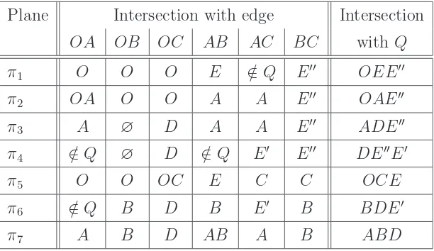
The intersections of the planes with the edges of Qc are in Table 1. The subscript c is omitted.

Plane Intersection with edge Intersection

OA OB OC AB AC BC with Q

π1 O O O E ∈/ Q E′′ _OEE′′

π2 OA O O A A E′′ _OAE′′

π3 A ∅ D A A E′′ ADE′′

π4 ∈/ Q ∅ _{D ∈/ Q E}′ _E′′ _DE′′_E′

π5 O O OC E C C OCE

π6 ∈/ Q B D B E′ _{B BDE}′

[image:18.612.161.467.35.212.2]

π7 A B D AB A B ABD

Table 1: Intersections of planes ofI_{with edges ofQ. A vertex ofQcontained inπj will show}

up three times in the row of πj. In order to clarify the geometry, we distinguish between a

plane’s meeting an edge line outside Q and not meeting it at all (i.e., their being parallel).

π2 π3 π4 π5 π6 π7

π1 x = 0 y = 2z

x+z = 1 2 y−z = 1 2

y = 1

x+ 2z = 1

z = 0

x =y

z = 2y−1

x = 2−3y

x+z = 1 3 y−z = 1 3

π2 y = 2z

x+z = 1₂

y = 2z x+y = 1

y = 2z x =z

y = 2z x+ 3z = 1

y = 2z

2x+ 3z = 1

π3 x = 0

z = 1₂ l356:

x+z = 1₂

y = 1₂

x+z = 1₂

y =z

π4 x = 1−2z

y = 1−z

x = 1−2z y =z

x = 1−2z y = 3z−1

π5 l356 x = 1−2y

z = 3y−1

π6 x = 0

y+z = 1

Table 2: The equations of the pairwise intersections of planes of I_c.

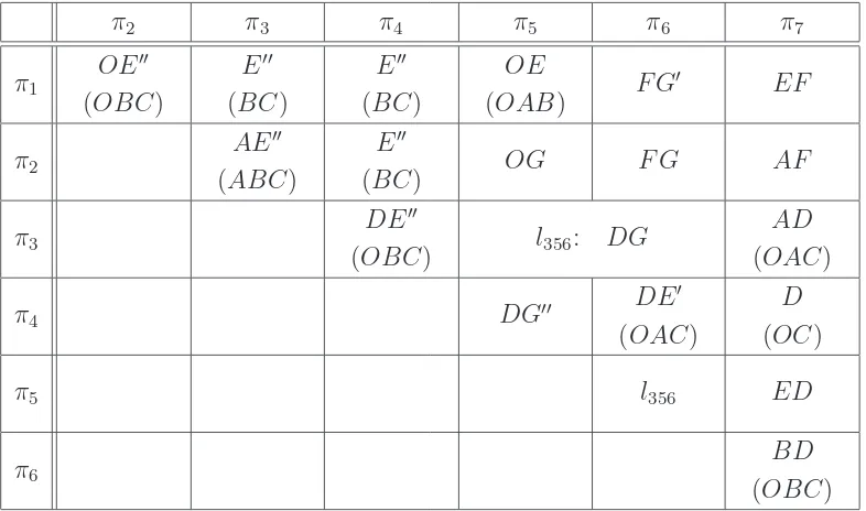
In Table 3 we describe the intersection of each line with Qc and with its interior. The

[image:18.612.83.582.308.540.2]

π2 π3 π4 π5 π6 π7

π1 OE

′′

(OBC)

E′′

(BC)

E′′

(BC)

OE

(OAB) F G

′ _EF

π2 AE

′′

(ABC)

E′′

(BC) OG F G AF

π3

DE′′

(OBC) l356: DG

AD

(OAC)

π4 DG′′ DE

′

(OAC)

D

(OC)

π5 l356 ED

π6 BD

[image:19.612.118.511.35.267.2]

(OBC)

Table 3: The intersections of lines withQ and Q◦_{. The second (parenthesized) row in each}

box shows the smallest face of Q to which the intersection belongs, if that is not Q itself; these intersections are not part of the intersection poset of (Q◦_,I).

Last, we need the intersection points of three planes ofI_{c; or, of a plane and a line. Some}

are not inQcat all; them we can ignore. Some are on the boundary ofQc; they are necessary in finding the denominator, but all of them are points already listed in (19). It turns out that

π2∩π5∩π7 =Hc

is the only vertex in Q◦

c, so it is the only one we need for the intersection poset.

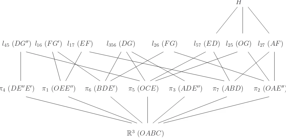
Here, then, is the intersection poset (Figure1). The subscript c is omitted. In the figure, for simplicity, we writeπj, etc., when the actual element is the simplexπj∩Q◦, etc.; we also

state the vertices of the simplex. The M¨obius function µ(ˆ0, u) equals (−1)codimu _{with the}

exception ofµ(ˆ0, l356) = 2.

4.1.4 Generating functions and the quasipolynomial

That was the first half of the work. The second half begins with finding rc(w) =E◦

(Q◦_c,Ic)(w)

from the Ehrhart generating functionsEu(t) of the intersections by means of (6). The next

R3 _(OABC)

π1 (OEE′′_{) π3 (ADE}′′_{) π2 (OAE}′′₎

π4 (DE′′_E′_{) π6 (BDE}′_{) π5 (OCE) π7 (ABD)}

l16 (F G′_{) l17 (EF) l356 (DG) l26 (F G) l57 (ED) l25 (OG) l27 (AF)}

l45 (DG′′₎

[image:20.612.80.567.53.290.2]

H

Figure 1: The intersection poset L_(Q◦_{,I) for semimagic squares. The diagram shows both}

the flats and (in parentheses) their intersections with Q.

result is:

−rc(1/x) = EOABC(x) +EOEE′′(x) +E_OAE′′(x) +EADE′′(x) +E_DE′_E′′(x) +E_OCE(x) +EBDE′(x) +E_ABD(x) +E_{F G}′(x) +EEF(x) +EOG(x) +EF G(x)

+EAF(x) + 2EDG(x) +EDG′′(x) +EDE(x) +EH(x)

= 1

(1−x)3_(1−x2₎ +

1

(1−x)(1−x2_)(1−x3₎+

1

(1−x)(1−x2₎2

+ 1

(1−x2₎3 +

1

(1−x2₎2_(1−x3₎+

1

(1−x)2_(1−x3₎

+ 1

(1−x)(1−x2_)(1−x3₎ +

1

(1−x)(1−x2₎2 +

1

(1−x3_)(1−x5₎

+ 1

(1−x3₎2 +

1

(1−x)(1−x4₎+

1

(1−x3_)(1−x4₎

+ 1

(1−x2_)(1−x3₎ + 2

1

(1−x2_)(1−x4₎+

1

(1−x2_)(1−x5₎

+ 1

(1−x2_)(1−x3₎ +

1 1−x5 .

Then by (16) the generating function for cubically counted semimagic squares is

Sc(x) = 72 x

2

(1−x)2rc(x)

= 72x

10_[18x9_{+ 46x}8_{+ 69x}7_{+ 74x}6_{+ 65x}5_{+ 46x}4_{+ 26x}3_{+ 11x}2_{+ 4x+ 1]}

(1−x2₎2_(1−x3₎2_(1−x4_)(1−x5₎ .

(21) From the geometrical denominator 60 or the (standard-form) algebraic denominator (1−

x60₎5 _{we know the period of S}

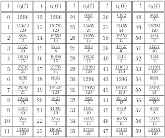
c(t) divides 60. We compute the constituents of Sc(t) by the

method of Section2.1; the result is that

Sc(t) =

        

3 10t

5₋ 75

8 t

4₊331

3 t

3₋5989

10 t

2_{+c1(t)t−c0(t), if t is even;}

3 10t

5₋ 75

8 t

4₊331

3 t

3₋11933

20 t

2_{+c1(t)t−c0(t), if t is odd;}

(22)

where c1 varies with period 6, given by

c1(t) =

        

1464, if t≡0,2 1456, if t≡4

2831

2 , if t≡1 2847

2 , if t≡3,5

(mod 6);

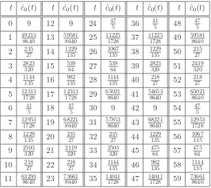
t c0(t) t c0(t) t c0(t) t c0(t) t c0(t)

0 1296 12 1296 24 6624 5 36

6192 5 48

6624 5

1 110413 120 13

120781 120 25

23465 24 37

23465 24 49

120781 120

2 3824 3 14

19552 15 26

18256 15 38

19552 15 50

3824 3

3 47727₄₀ 15 9315₈ 27 9315₈ 39 47727₄₀ 51 44271₄₀

4 18152₁₅ 16 16856₁₅ 28 18152₁₅ 40 3544₃ 52 3544₃

5 25705₂₄ 17 25705₂₄ 29 131981₁₂₀ 41 121613₁₂₀ 53 131981₁₂₀

6 6192₅ 18 6624₅ 30 1296 42 1296 54 6624₅

7 25193₂₄ 19 129421₁₂₀ 31 119053₁₂₀ 43 129421₁₂₀ 55 25193₂₄

8 19552 15 20

3824 3 32

3824 3 44

19552 15 56

18256 15

9 44847 40 21

41391 40 33

44847 40 45

8739 8 57

8739 8

10 3544 3 22

3544 3 34

18152 15 46

16856 15 58

18152 15

[image:22.612.147.475.34.308.2]

11 130253₁₂₀ 23 140621₁₂₀ 35 27433₂₄ 47 27433₂₄ 59 140621₁₂₀

Table 4: Constant terms (without the negative sign) of the constituents of the semimagic cubical quasipolynomial Sc(t).

The principal constituent (for t ≡0) is

3 10t

5₋ 75

8 t

4₊ 331

3 t

3₋ 5989

10 t

2_{+ 1464t−1296.}

Its unsigned constant term, 1296, is the number of order types of semimagic squares. Al-lowing for the 72 symmetries of a semimagic square, there are just 18 symmetry classes of order types.

For the first few nonzero values ofSc(t) see the following table. (This is sequenceA173546 in the OEIS [15].) The third row is the number of normalized squares, or symmetry classes (sequence A173723), which equals Sc(t)/72. The other lines give the numbers of reduced squares (sequenceA173727) and of reduced normal squares (i.e., symmetry types of reduced squares; sequence A173724), which may be of interest.

t 8 9 10 11 12 13 14 15 16 17 18 19

Sc(t) 0 0 72 288 936 2592 5760 11520 20952 35712 57168 88272

sc(t) 0 0 1 4 13 36 80 160 291 496 794 1226

Rc(t) 72 144 432 1008 1512 2592 3672 5328 6696 9648 11736 15552

rc(t) 1 2 6 14 21 36 51 74 93 134 163 216

the quasipolynomial, provide additional verification of the correctness of the counts and constituents.

4.1.5 Another method: Direct counting

We checked the constituents by directly counting (in Maple) all semimagic squares for

t≤100. The numbers agreed with those derived from the generating function and quasipoly-nomial above.

4.2

Semimagic squares: Affine count (by magic sum)

Now we count squares by magic sum: we computeSa(t), the number of squares with magic sum t.

4.2.1 The Birkhoff polytope

The polytope P for semimagic squares of order 3, counted by magic sum, is 4-dimensional and integral. (It is the polytope of doubly stochastic matrices of order 3, i.e., a Birkhoff polytope [8, 4].)

4.2.2 Affine weak semimagic

The polytope for weak semimagic squares of order 3 is the same P.

The weak quasipolynomial, or rather, polynomial, first computed by MacMahon [12, Vol. II, par. 407, p. 161], is

t4_−6t3 _{+ 15t}2_{−18t+ 8}

8 =

(t−1)(t−2)(t2_{−3t+ 4)}

8

with generating function

6x4_−9x3 _{+ 10x}2_{−5x+ 1}

(1−x)5 .

4.2.3 Reduction

The count is via Ra(s), the number of reduced squares with magic sum s. The formula is

Sa(t) = X

0<s≤t−3

s≡t(mod 3)

Ra(s) if t >0. (23)

We have Ra(s) = 72ra(w), where ra(s) is the number of reduced, normalized squares with magic sums, equivalently the number of 1

s-integral points in the interior of the 3-dimensional

polytopeQa defined by

0≤x, y; 0≤z ≤y; x+y≤ 1

with the seven excluded (hyper)planes

z = y−x 2 ,

y

2,

1−y−2x

2 ,

1−x−y

2 , y−x, 1−x−2y, 1−2x−2y , (25)

the three coordinates beingx=α/s, y=β/s, and z =δ/s.

The hyperplane arrangement for reduced, normalized squares is that of (25). We call it

I_{a. Thus ra(s) =E}◦

Q◦_a,Ia(s).

4.2.4 The reduced, normalized weak polytopal quasipolynomial

This function simply counts 1

s-lattice points in Q ◦

a. The counting formula is

P

α

P

β

P

δ1,

summed over all triples that satisfy (14). It simplifies to

X

α

⌊s−1 2 ⌋ −α

2

,

which gives the Ehrhart quasipolynomial

EQ◦_a(s) =

⌊s−1 2 ⌋

3

=

          

s−1 2

3

= ₄₈1(s−1)(s−3)(s−5), for odds;

s−2 2

3

= ₄₈1(s−2)(s−4)(s−6), for even s.

(26)

The leading coefficient is volQa. We deduce from (26) that

EP◦(x) =

x7_{(1 +x)}

(1−x2₎4

and by reciprocity that

EP(x) =

1 +x

(1−x2₎4.

4.2.5 Geometrical analysis of the reduced, normalized polytope

We apply M¨obius inversion, Equation (6), over the intersection poset L_(Q◦

a,I).

We number the planes:

The intersection of two planes, πj ∩πk, is a line we call ljk; π3∩π5 ∩π6 is a line we also

call l356. The intersection of three planes is, in general, a point but not usually a vertex of (Qa,I_{a). Our geometrical notation is as in the cubical analysis.}

We need to find the intersections of the planes with Q◦

a, separately and in combination.

Here is a list of significant points; we shall see it is the list of vertices of (Qa,I_{a). The first}

column has the vertices ofQa, the second the vertices of (Qa,I_{a) that lie in open edges, the}

third the vertices that lie in open facets, and the last is the sole interior vertex.

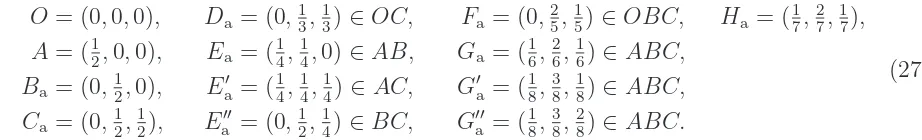
O = (0,0,0), Da = (0,1₃,1₃)∈OC, Fa = (0,2₅,1₅)∈OBC, Ha = (1₇,2₇,1₇), A= (1₂,0,0), Ea = (1₄,1₄,0)∈AB, Ga = (1₆,2₆,1₆)∈ABC,

Ba = (0,1₂,0), E′

a = (14, 1 4,

1

4)∈AC, G

′

a = (18, 3 8,

1

8)∈ABC, Ca = (0,1₂,1₂), E′′

a = (0,12, 1

4)∈BC, G

′′

a = (18, 3 8,

2

8)∈ABC.

(27)

The least common denominator of O, A, Ba, Ca explains the period 2 of EQ◦_a. The denom-inator of (Qa,I_{a) is the least common denominator of all the points; it evidently equals}

8·3·5·7 = 840.

The intersections of the planes with the edges of Qa are in Table 1. Table 5 shows the

lines generated by pairwise intersection of planes. Table 3describes the intersection of each line with Qa and with Q◦

a.

π2 π3 π4 π5 π6 π7

π1 x = 0 y = 2z

x = 1−4z

3 y = 1+2z

3

x+ 2z = 1₂

y = 1₂

x =y z = 0

x = 2−5y z = 3y−1

x = 1−5z

4 y = 1+3z

4

π2 x+y =

1 2 y = 2z

x = 1−2y y = 2z

x =z y = 2z

x = 1−5z y = 2z

x = 1−5z

2 y = 2z

π3

x = 0

y = 1−2z l356:

x+z = 1₃

y = 1₃

2x+ 3y = 1

z =y

π4

x = 3y−1

z = 1−2y

x = 1−3y z =y

x+y = 1 3 z = 1₃

π5 l356

x = 1−3y z = 4y−1

π6 x = 0

[image:25.612.82.543.148.218.2]

z = 1−2y

Table 5: The equations of the pairwise intersections of planes of I_a.

Last, we need the intersection points of three planes ofI_{a; or, of a plane and a line. Some}

that

π2∩π5∩π7 =Ha

is the only vertex in Q◦

a, so it is the only one we need for the intersection poset.

The combinatorial structure and the intersection poset (Figure 1) for the affine count are identical to those for the cubical count. The reason is that the affine polytope Pa is the 4-dimensional section of Pc by the flat in which the magic sum equals 1, and this flat is orthogonal to the line of intersection of the whole arrangement H_a.

4.2.6 Generating functions and the quasipolynomial

The second half of the affine solution is to findra(s) =E◦(Q◦_a,Ia)(s) by applying Equations (1)–

(4) after finding the Ehrhart generating functions Eu(s) for u ∈ L(Q◦_a,Ia). The next step,

then, is to calculate those generating functions. This is done by LattE. Then (−1)3_ra(x−1₎

is the sum of all these rational functions; that is,

−ra(1/x) = EOABC(x) +EOEE′′(x) +E_OAE′′(x) +EADE′′(x) +E_DE′′_E′(x) +E_OCE(x) +EBDE′(x) +E_ABD(x) +E_{F G}′(x) +EEF(x) +EOG(x) +EF G(x)

+EAF(x) + 2EDG(x) +EDG′′(x) +EDE(x) +EH(x)

= 1

(1−x)(1−x2₎3 +

1

(1−x)(1−x4₎2 +

1

(1−x)(1−x2_)(1−x4₎

+ 1

(1−x2_)(1−x3_)(1−x4₎ +

1

(1−x3_)(1−x4₎2 +

1

(1−x)(1−x2_)(1−x4₎

+ 1

(1−x2_)(1−x3_)(1−x4₎ +

1

(1−x2₎2_(1−x3₎ +

1

(1−x5_)(1−x8₎

+ 1

(1−x4_)(1−x5₎+

1

(1−x)(1−x6₎+

1

(1−x5_)(1−x6₎

+ 1

(1−x2_)(1−x5₎+ 2

1

(1−x3_)(1−x6₎+

1

(1−x3_)(1−x8₎

+ 1

(1−x3_)(1−x4₎+

1 1−x7 .

(28) The generating function for the affine count of semimagic squares, by (23), is

Sa(x) = 72 x

3

1−x3 ra(x) =

72x15

(

18x21+ 5x20+ 15x19+ 11x17−8x16+x15−23x14−13x13−22x12−9x11

−16x10+x9−3x8+ 7x7+ 7x6+ 9x5+ 7x4+ 6x3+ 4x2+ 2x+ 1

)

(1−x3₎2_(1−x4_)(1−x5_)(1−x6_)(1−x7_)(1−x8₎ .

From the geometrical or generating-function denominator we know that the period of

Sa(t) divides 840 = lcm(3,4,6,7,8). This is long, but it can be simplified. The factor 7 in the period is due to a single term in (28). If we treat it separately we have ra as a sum of the H-term x7_/(1−x7_{) and a “truncated” generating function for r}

a(x) + x

7

1−x7, and a

corresponding truncated expression

Sa(x)−72

x10

(1−x3_)(1−x7₎ =

−72x10

(

17x19+ 5x18+ 15x17+x16+ 12x15−7x14+ 2x13−7x12

−8x11−9x10−9x9−6x8−6x7−x6+x4 +x3−1

)

(1−x3₎2_(1−x4_)(1−x5_)(1−x6_)(1−x8₎ .

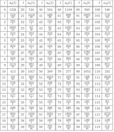
We extract the constituents from this expression as in Section 2.1, separately for the two parts of the generating function. The constituents are all of the form

Sa(t) = 1 8t

4 ₋9

2t

3_+a2(t)t2_{−a1(t)t+a0(t)−72S7(t), (30)}

where S7(t) is a correction, to be defined in a moment, and

a2(t) =

         243

4 , if t≡0 218

4 , if t≡1,5 227

4 , if t≡2,4 234

4 , if t≡3

(mod 6);

a1(t) =

                             1968

5 , if t≡0 1158

5 , if t≡1,5 1383

5 , if t≡2,10 1653

5 , if t≡3 1428

5 , if t≡4,8 1923

5 , if t≡6 1113

5 , if t≡7,11 1698

5 , if t≡9

(mod 12);

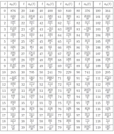
and a0(t) is given in Table 6.

We call the constituents of the quasipolynomial

Sa(t) + 72S7(t) = 1 8t

4₋ 9

2t

3_+a2(t)t2_{−a1(t)t+a0(t)}

the truncated constituents of Sa(t), since they correspond to the truncated generating

func-tion menfunc-tioned just above. The S7 term that undoes the truncation is

S7(t) :=

t−1 21

+

(

= t−¯t

21 +s7(t),

where ¯t:= the least positive residue of t modulo 7 and

s7(t) :=

(

1, if t≡10,13,16,17,19,20 (mod 21); 0, otherwise.

Note that ¯t = 21 if t≡0, so that S7(0) =−1 and in general S7(21k) =k−1.

t a0(t) t a0(t) t a0(t) t a0(t) t a0(t) t a0(t)

0 1224 20 524 40 584 60 1188 80 560 100 548

1 7259 40 21 31419 40 41 6299 40 61 8699 40 81 29979 40 101 7739 40

2 1801₅ 22 1741₅ 42 5121₅ 62 1621₅ 82 1921₅ 102 4941₅

3 23067₄₀ 23 827₄₀ 43 347₄₀ 63 24507₄₀ 83 −613 40 103

1787 40

4 2452₅ 24 5832₅ 44 2332₅ 64 2632₅ 84 5652₅ 104 2512₅

5 2239₈ 25 2143₈ 45 6975₈ 65 1951₈ 85 2431₈ 105 6687₈

6 4653₅ 26 1513₅ 46 1453₅ 66 4833₅ 86 1333₅ 106 1633₅

7 5243 40 27 26523 40 47 4283 40 67 3803 40 87 27963 40 107 2843 40 8 2224 5 28 2164 5 48 5544 5 68 2044 5 88 2344 5 108 5364 5 9 31131 40 29 8891 40 49 8411 40 69 32571 40 89 7451 40 109 9851 40

10 413 30 1017 50 389 70 377 90 1053 110 353

11 539₄₀ 31 2939₄₀ 51 24219₄₀ 71 1979₄₀ 91 1499₄₀ 111 25659₄₀

12 5796₅ 32 2656₅ 52 2596₅ 72 5976₅ 92 2476₅ 112 2776₅

13 7547₄₀ 33 28827₄₀ 53 6587₄₀ 73 6107₄₀ 93 30267₄₀ 113 5147₄₀

14 1477₅ 34 1777₅ 54 4797₅ 74 1657₅ 94 1597₅ 114 4977₅

15 5823 8 35 799 8 55 1279 8 75 5535 8 95 1087 8 115 991 8 16 2488 5 36 5508 5 56 2368 5 76 2308 5 96 5688 5 116 2188 5 17 8603 40 37 11003 40 57 32283 40 77 10043 40 97 9563 40 117 33723 40 18 4689 5 38 1189 5 58 1489 5 78 4509 5 98 1369 5 118 1309 5

[image:28.612.123.503.152.592.2]

19 2651₄₀ 39 26811₄₀ 59 1691₄₀ 79 4091₄₀ 99 25371₄₀ 119 3131₄₀

Table 6: Constant terms of the truncated constituents of Sa(t).

The principal constituent of Sa(t) (that is, for t≡0) is

1 8t

4₋9

2t

3₊ 243

4 t

2₋ 13896

35 t+ 1296.

(This incorporates the effect of the term −72S7.) The constant term is the same as in the cubic count, as it is the number of order types of semimagic squares.

We give the first few nonzero values of Sa(t) in the following table. (This sequence is A173547in the OEIS [15].) The third row is the number of normalized squares, or symmetry classes (sequence A173725); this is Sa(t)/72. The last rows are the numbers of reduced squares (sequence A173728) and of reduced, normalized squares (sequence A173726) with magic sum t.

t 12 13 14 15 16 17 18 19 20 21 22 23 24

Sa(t) 0 0 0 72 144 288 576 864 1440 2088 3024 3888 5904

sa(t) 0 0 0 1 2 4 8 12 20 29 42 54 82

Ra(t) 72 144 288 504 720 1152 1512 2160 2448 3816 3960 5544 6264

ra(t) 1 2 4 7 10 16 21 30 34 53 55 77 87

4.2.7 Alternative methods: Direct counting and direct computation

We verified our formulas by computingSa(t) for t≤100 through direct enumeration of nor-mal squares. The results agree with those computed by expanding the generating function. We also applied Proposition 1 to derive a formula, independent of all other methods, by which we calculated numbers (which we are not describing; see the “Six Little Squares” Web page [7]) that allowed us to find the 840 constituents by interpolation. These interpolated constituents fully agreed with the ones given above.

5

Magilatin squares of order 3

A magilatin square is like a semimagic square except that entries may be equal if they are in different rows and columns. The inside-out polytope is the same as with semimagic squares except that we omit those hyperplanes that prevent equality of entries in different rows and columns. Thus, in our count of reduced squares, we have to count the fractional lattice points in some of the faces of the polytope.

The reduced normal form of a magilatin square is the same as that of a semimagic square except that the restrictions are weaker. It might be thought that this would introduce ambiguity into the standard form because the minimum can occur in several cells, but it turns out that it does not.

Proposition 2. A reduced, normal 3×3 magilatin square has the form (13) with the re-strictions

0< β, γ; 0≤α; 0≤δ≤β;

and (15). Each reduced square with w in the upper right corner corresponds to exactly t−w−1 different magilatin squares with entries in the range (0, t), for 0 < w < t. Each reduced square with magic sum s corresponds to one magilatin square with magic sum equal to t, if t≡s (mod 3), and none otherwise, for 0< s < t.

Proof. The proof is similar to that for semimagic squares; we can arrange the square by permuting rows and columns and by reflection in the main diagonal so that x11 is the smallest entry, the first row and column are each increasing, andx21 ≥x12. We cannot say

x21> x12 because entries that do not share a row or column may be equal. Still, we obtain

the form (13) with the bounds (31) and the same inequations (15) as in semimagic because all the latter depend on having no two equal values in the same line (row or column).

Each reduced, normal magilatin square gives rise to a family of true magilatin squares by adding a positive constant to each entry and by symmetries, which are generated by row and column permutations and reflection in the main diagonal. Call the set of symmetries

G_{. As with semimagic, |}G_{| = 2(3!)}2 _{= 72. Each normal, reduced square S gives rise to}

|G_/G_{S| = 72/|}G_{S| squares via symmetries, where} G_{S is the stabilizer subgroup of S. If all}

entries are distinct, then the square is semimagic, G_{S is trivial, and everything is as with}

semimagic squares. However, if α = 0 or δ = 0 or δ = β, the stabilizer is nontrivial. We consider each case in turn.

The case α= 0< δ. Hereδ < β because no line can repeat a value. To fix the square we cannot permute any rows or columns but we can reflect in the main diagonal, so |G_{S| = 2.}

Moreover, (15) reduces to

δ6=γ,β

2,

β+γ

2 .

We are in OBC, the x = 0 facet of Q, with the induced arrangement of three lines, Ix=0_.

The number of reduced magilatin squares of this kind is 36rOBC(t), where rOBC(t) is the

number of 1

t-lattice points in the open facet and, equivalently, the number of symmetry types

of reduced magilatin squares of this kind. We apply Equations (1)–(4) to the intersection poset L_(OBC◦_,Ix=0_{), which is found in Figure 2. The M¨obius function µ(OBC, u) equals}

(−1)codimu_.

The case δ = 0< α. In this case a nontrivial member of G_{S can only exchange the two}

zero positions. Such a symmetry that preserves the increase of the first row and column is unique (as one can easily see); thus |G_{S|= 2. Furthermore, (15) reduces to}

α 6=β.

We are inOAB, thez = 0 facet, with the induced arrangementIz=0 _{of one line. The number}

of reduced magilatin squares of this kind is 36rOAB(t), where rOAB(t) is the number of 1_t

-lattice points in the open facet and, equivalently, the number of symmetry types of reduced squares. We apply Equations (1)–(4) to the intersection poset L_(OAB◦_,Iz=0_{), shown in}

Figure2. The M¨obius function µ(OAB, u) equals (−1)codimu_.

The case δ = β. Here we must have α > 0. There are two zero positions in opposite corners. A symmetry that exchanges them and preserves increase in the first row and column is uniquely determined, so |G_{S|= 2. The inequations reduce to}

We are in OAC, the facet where y = z, with the two-line induced arrangement Iy=z_{. The}

number of reduced magilatin squares of this kind is 36rOAC(t), whererOAC(t) is the number

of 1_t-lattice points in the open facet, equally the number of reduced symmetry types. We apply Equations (1)–(4) to the intersection poset L_(OAC◦_,Iy=z_{) in Figure 2. The M¨obius}

function µ(OAC, u) equals (−1)codimu_.

The case α = 0 = δ. In these squares there are three zero positions and the whole square is a cyclic latin square. Any symmetry that fixes the zero positions also fixes the rest of the square. There are 3! symmetries that permute the zero positions, generated by row and column permutations. They all preserve the entire square. Therefore |G_{S| = 6. The}

inequations disappear. We are in the edgeOB, which is the face where x=z = 0, with the empty arrangement, Ix=z=0 _{= ∅. The number of reduced magilatin squares of this kind is}

12rOB(t), where rOB(t) is the number of 1_t-lattice points in the open edge, also the number

of reduced symmetry types. The intersection poset L_(OB◦

,∅_{) consists of the one element} OB, whose M¨obius functionµ(OB, OB) = 1.

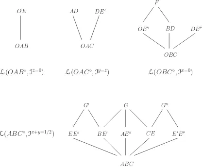
To get the intersection posets we may examine Tables 1 and 3 to find the edges and vertices of (Q◦

,I_{) in each closed facet. We also need to know which vertex is in which edge;}

this is easy. Although we do not need the fourth facet, ABC, we include it for the interest of its more complicated geometry.

Of course all the functions rs and Rml depend on whether we are counting cubically or affinely (thus, subscripted c or a); the two types will be treated separately. But the general conclusions hold that

Rml(x) = 72rs(x) + 36[rOAB(x) +rOAC(x) +rOBC(x)] + 12rOB(x), (32)

and for the number of reduced symmetry types, rml(t) with generating functionrml(x),

rml(x) = rs(x) +rOAB(x) +rOAC(x) +rOBC(x) +rOB(x), (33)

where rs(x) is from semimagic and, by Equation (4) since |µ(X, Y)| = 1 for every lower interval in each facet poset (except facetABC, which we do not use),

(−1)3rOAB(1/x) =EOAB(x) +EOE(x),

(−1)3rOAC(1/x) =EOAC(x) +EAD(x) +EDE′(x),

(−1)3rOBC(1/x) =EOBC(x) +EOE′′(x) +E_BD(x) +E_DE′′(x) +E_F(x), (−1)2_r

OB(1/x) =EOB(x);

(34)

the sign and reciprocal on the left result from Equation (6).

There is also the generating function of the number of cubical or affine symmetry classes,

l(t), whose generating function isl(x). This is obtained from rml(t) in the same way as L(t) is from Rml(t), the exact way dependin