Electronic Journal of Qualitative Theory of Differential Equations 2011, No. 20, 1-11;http://www.math.u-szeged.hu/ejqtde/
Attractors and basins of dynamical systems
Attila D´enes, G´eza Makay
Abstract
There are several programs for studying dynamical systems, but none of them is very useful for investigating basins and attractors of higher dimensional systems. Our goal in this paper is to show a new algorithm for finding even chaotic attractors and their basins for these systems. We present an implementation and examples for the use of this program.
Key words: dynamical systems, attractors, basins, numerical methods.
2000 Mathematics Subject Classification: Primary 37D45, 37M99.
1
Introduction
There exist several program packages for investigating dynamical systems. However, we found that even the most widespread of these are not suitable for the examination of attractors and basins of dynamical systems. For ex-ample, Dynamica written in Mathematica [2] does not contain a procedure for representing attractors and basins. Dynamics[1] does have such a proce-dure, but as it was written under DOS, it is rather difficult to use on today’s computers, and the algorithm has some inadequacies that – in some cases – can cause imperfect results. For this reason we established a new algorithm and its computer realization to find and visualize attractors and basins of discrete and continuous dynamical systems.
2
Dynamical systems
Definition 2.1. Let X ⊂ Rn and Y ⊂ R. The pair (X, π) is called a
dynamical system if the map π :X×Y →X has the following properties:
• π(x,0) =x for any x∈X (identity axiom),
• π(π(x, t), s) = π(x, t+s) for any x∈X and t, s∈Y (group axiom),
• π is continuous on X×Y.
Given a dynamical system on X, the space X is called phase space, π
is called phase map and Y stands for time. Usually Y = R or Y = Z. In the first case we have a continuous dynamical system, in the second case a discrete dynamical system.
Definition 2.2. LetF be a map from the n-dimensional space to itself. We say that a compact set A ∈ Rn
is an attractor for the map F if it satisfies the following properties:
• F(A) =A, i. e.A is invariant,
• Acontains an initial point whose trajectory travels throughoutA, i. e. it is dense in A,
• initial points starting close to A have trajectories that stay close to A and tend asymptotically to A.
The basin of an attractor is the set of initial points whose trajectories tend to the attractor.
3
The algorithm of
Dynamics
The routineBasins and AttractorsofDynamicsis designed for 2-dimensional phase spaces. When the phase space has dimension higher than two, one can use the routine Basins and Attractors 2. This algorithm does all its calculations using 2-dimensional projections defined by the axes, which will certainly cause inaccuracies.
infinity, i. e. the points whose trajectories diverge. The basin of the 2nth attractor is coloured using colour 2n+ 1.
Initially all grid boxes are uncoloured, but as the routine proceeds all grid boxes will be coloured. The routine selects an uncoloured box and examines the trajectory that starts at the center of the grid box. In the case of discrete dynamical systems the routine starts to iterate the difference equation, in the continuous case it iterates the time-one map. The colour of the box will be determined by colours of the boxes encountered by this trajectory. Let C1 denote the first positive even number not currently used for colouring any grid boxes. As long as the trajectory does not encounter a previously coloured trajectory, the algorithm will use the colours C1 and C1 + 1. The selected box will be temporarily given the colour C1 + 1 and the method starts to iterate the point at the center of the box. As long as the trajectory passes through uncoloured boxes, all the boxes encountered by the trajectory will be coloured with colour C1 + 1 as well. Proceeding with the iteration the trajectory has to encounter a previously coloured box or it has to diverge. For the colouring the algorithm uses the following rules for the different cases below:
1. The trajectory diverges. We cannot check rigorously whether a tra-jectory really tends to infinity, so this method says that a tratra-jectory diverges if it leaves the screen area and gets far enough from it. Then all the boxes coloured with colour C1 or C1+ 1 are changed to colour 1 and the routine stops iterating this trajectory.
2. While the routine is still plotting uncoloured boxes using colourC1+ 1, the trajectory encounters boxes coloured by C2 on a given number of consecutive iterates, where the number C2 is odd and C2 < C1. This means that there is another trajectory that passes together with the actual trajectory for a given number of consecutive steps and the algorithm assumes that these two trajectories will remain near to each other and tend to the same attractor, so the routine stops iterating and all the boxes coloured C1+ 1 are changed to colour C2.
3. While the routine is plotting uncoloured boxes using colour C1, the trajectory encounters boxes coloured by C2 on a given number of con-secutive iterates, where the number C2 is odd and C2 < C1. In this case the method does not change the colours, it goes on iterating, as an attractor can be near to basins of other attractors.
4. The trajectory encounters a box coloured C3, where C3 is even and
another trajectory that passes together with the actual trajectory for a given number of consecutive steps. The iteration is terminated and all points coloured C1 and C1+ 1 are changed to the basin colour C3+ 1. 5. The trajectory encounters a box that it has previously coloured C1+ 1 and passes along with it for a given number of iterations, the routine switches to the colour C1, because it assumes that from this point on the trajectory is in the attractor. Uncoloured boxes and boxes coloured
C1+ 1 that the trajectory encounters after this will be coloured C1. If none of the cases 1, 2, 3, or 4 occurs, then 5 must occur, and the program will eventually get to a point where the trajectory does not pass through uncoloured boxes and boxes colouredC1+1. In the case of a chaotic attractor this may even require thousands of iterates. At this point, the routine stops iterating the trajectory and selects the next uncoloured box for which the whole process is repeated, until there are no uncoloured boxes.
4
The new algorithm
The routine of Dynamicshas several drawbacks:
• Since all computation is done on 2-dimensional projections, there is a
possibility that different trajectories are merged.
• The grid size is determined by the resolution of the screen (the pixel
size), the program cannot compute accurately enough to get more pre-cise results.
• The method colors grid boxes, which does not allow different
trajecto-ries, basins and attractors to be near one another.
• The algorithm does not actually follow the trajectories, it simply relies
on the colouring of grid boxes, and assumes that if we pass through boxes of the same colour, then we follow a trajectory, but this might also be proven false.
Our method tries to resolve these problems.
save the point itself in order to know the full trajectory. For colouring we use numbers, as it was done in Dynamics. If the trajectory gets far enough from the domain under examination, we say that it diverges and give it the colour of the basin of infinity. Otherwise, if the point lies in the domain un-der examination, we examine all the points near our actual point, i. e. all the points that fall into the same box or any of the neighbouring boxes. If there is no point to which our actual point remains near during a given number of steps, we continue the iteration and examine the near points again. If we find a point such that its iterates remain near to the iterates of our actual point for this given number of steps, we stop iterating and give a colour to the actual trajectory according to the trajectory of the near point we have found.
1. If the found point is a point of the actual trajectory, we give the trajec-tory the smallest odd colour not yet used and we also store the point which we first reencountered: from this point on we colour the trajec-tory with the colour of the attractor. Then we continue iterating long enough in order to find the complete attractor. To avoid identifying different parts of an attractor (lying far from each other) as different attractors, we make a test on this “new” attractor found. We compare the new attractor with all the previously found attractors: if they have enough common points, we verify whether these points remain near to each other after several iterations. If we discover a previously found attractor with this property, we give our actual trajectory the colours of this previously found attractor and basin.
2. If the found point is not a point of the actual trajectory, we give the colour of the found point to our actual trajectory.
The main advantage of the new algorithm is that we only test the points that are really near to the actual trajectory: this is the only reason to use the grid boxes. In contrary to the algorithm of Dynamics, which assigns one colour to each grid box, we do not colour the grid boxes, but rather the points themselves. This provides a more accurate image as several attractors and basins can have points in the same grid box. Also, our algorithm can be applied for dynamical systems of arbitrary dimension.
5
Some notes on the program
The first version of the program based on this algorithm was written in
the program in Visual C++. This new program has several features that facilitate the examination of dynamical systems. The development of the program is in the final stage, but it is already applicable for research.
After starting the procedure we give the dimension of the system, the grid size, the number of iterates for which we require the actual trajectory to remain near the trajectory it encounters, the starting and ending points of the area under examination and the equations for each dimension. The equations given by the user are parsed by a built-in syntactic and semantic parser. The resulting internal structure is interpreted whenever the computation needs it. Arbitrary projection of then-dimensional space into two dimensions can be represented using the user-given expressions, that are parsed by the same built-in procedure. When the program has finished computing, the figure appears: we can choose which basin(s) or attractor(s) we would like to be represented, and we can also change the size of the points both for the attractors and the basins. In the left bottom corner of the picture we can read the position of the mouse pointer, we can move and magnify the image. The resulting figure can be saved in two different ways: in a special format which preserves the results of the calculation or in an EPS file.
6
Examples
6.1
The H´
enon map
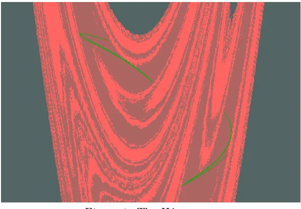
Figure 1 shows the strange attractor of the famous H´enon map [1].
Figure 1. The H´enon map
6.2
The Bogdanov map
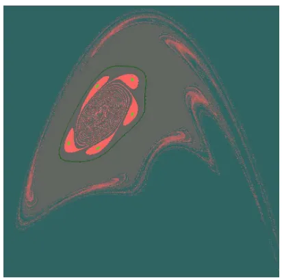
Figure 2 shows the attractors of the Bogdanov map [3] and their basins.
x′
1 =x1 +x2+ 0.0025x2+ 1.44x1(x1 −1)−0.1x1x2
x′
2 =x2 + 0.0025x2+ 1.44x1(x1−1)−0.1x1x2
This map has four attractors. Figure 2 suggests that there is an area around the origin in which the basins of two of the four attractors are dense. Dy-namics does not recognize this phenomenon as it identifies this area as the basin of the closed curve (see Figure 3). Moreover, the attractor marked with green is not continuous as it should be and the attractor consisting of five points (inside the closed curve) is represented as five closed curves because of the extraordinarily slow spiraling convergence to the attractor.
Figure 2. The Bogdanov map
This example shows the danger of using 2-dimensional projections: Dy-namicsonly finds one attractor of this map [1]; in fact there are two attractors with the same 2-dimensional projection. Our program finds both attractors.
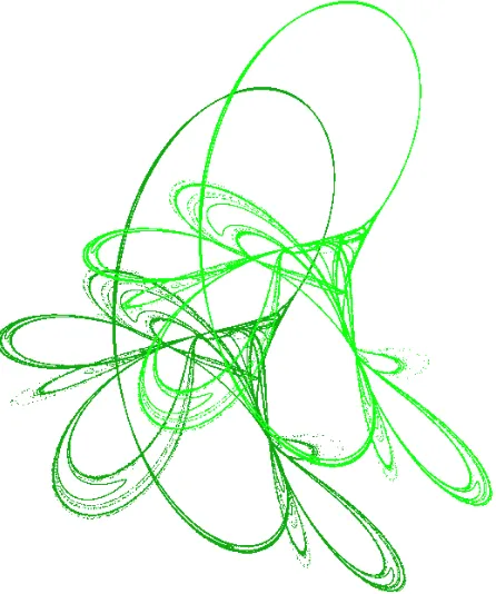
Figure 4. Three-dimensional Tinkerbell map
6.4
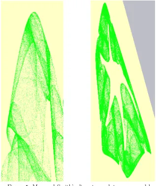
A discrete predator–prey model by Maynard Smith
Figure 5 shows a part of the attractor, and the whole attractor of a discrete predator–prey model initiated by Maynard Smith [4].
x′
1 = 3.6545x1(1−x1)−x1x2
x′
2 =
1 0.31x1x2
Figure 5. Maynard Smith’s discrete predator-prey model
Acknowledgments. Supported by the Hungarian National Foundation for Scientific Research (OTKA K75517) and by the T ´AMOP-4.2.2/08/1/2008-0008 program of the Hungarian National Development Agency
References
[1] Nusse, H. E., Yorke, J. A.,Dynamics: Numerical Explorations, Springer-Verlag, 1998.
[3] Djellit, I., Boukemara, I.Bifurcations and Attractors in Bogdanov Map, Vis. Math. 6, No. 4 (2004)
[4] Koc¸ak, H. Differential and difference equations through computer experi-ments, Springer-Verlag, 1989.
Attila D´enes, SZTE, Bolyai Institute, Aradi v´ertan´uk tere 1, H-6720, Hungary ([email protected])
G´eza Makay, SZTE, Bolyai Institute, Aradi v´ertan´uk tere 1, H-6720, Hungary ([email protected])