On the One Class of Hyperbolic Systems
⋆Vsevolod E. ADLER and Alexey B. SHABAT L.D. Landau Institute for Theoretical Physics,
1A prosp. ak. Semenova, 142432 Chernogolovka, Russia
E-mail: [email protected], [email protected]
Received October 27, 2006; Published online December 27, 2006
Original article is available athttp://www.emis.de/journals/SIGMA/2006/Paper093/
Abstract. The classification problem is solved for some type of nonlinear lattices. These lattices are closely related to the lattices of Ruijsenaars–Toda type and define the B¨acklund auto-transformations for the class of two-component hyperbolic systems.
Key words: hyperbolic systems; B¨acklund transformations; Ruijsenaars–Toda lattice; dis-crete Toda lattice
2000 Mathematics Subject Classification: 35L75; 35Q55; 37K10; 37K35
This paper is dedicated to the memory of Vadim Kuznetsov
1
Introduction
In this paper we solve the problem of classification of the consistent pairs of the lattices
ux=F(u1, u, v), vx=G(u, v, v−1), (1)
uy =P(u−1, u, v), vy =Q(u, v, v1). (2)
Hereu=u(n, x, y),v=v(n, x, y),n∈Zand subscripts denote both the partial derivatives with respect tox, y and the shift with respect ton. The nondegeneracy conditions are assumed
FvFu1GuGv−1PvPu
−1QuQv1 6= 0. (3)
Due to the conditionFv 6= 0, the first equation of the lattice (1) can be solved with respect to the
variable v, then the second equation of the lattice rewrites as a lattice of the Ruijsenaars–Toda type [1,2,3,4]
uxx=A(u1,x, ux, u−1,x, u1, u, u−1) (4)
while its symmetry takes the form
uy =B(ux, u1, u, u−1). (5)
Clearly, the roles of xandy may be interchanged and equation (4) may be replaced by a lattice of the form
uyy=C(u1,y, uy, u−1,y, u1, u, u−1). (6)
The classification problem for the lattices (4) was solved, in a different setting, in our paper [5], see also [6,7, 8,9]. The approach based on the relation to the lattices (1) allows to reproduce
this result in a slightly more general way and is promising for further generalizations. The classification of the integrable lattices of the form (1) was obtained by Yamilov [13]. The main postulate in his work was that, instead of (2), a symmetry of a high enough order exists, and moreover, the lattice was assumed to be Hamiltonian. Our aim here is to obtain the answer under the minimal restrictions. However, in comparison with the result of Yamilov, our list contains only two more pairs. These pairs are not Hamiltonian, and they are reducible in some definite sense. We discuss these curious examples separately in Section 5.
The interest to the lattices (1) is explained by their close relation to many other integrable models, see e.g. [10,11,12]. The higher symmetries of such lattices generate the hierarchies of the evolution systems of the nonlinear Schr¨odinger type. In this context equation (2) defines the first negative flow of the hierarchy and corresponds to some hyperbolic system, see Sec-tion 4.1. Although not all integrable two-component hyperbolic systems can be obtained in this way, this correspondence is a source of important examples. Also, the linear combinations of the flows (1), (2) constitute a class of equations containing Ablowitz–Ladik and Sklyanin lattices [14,15].
In Section4.3we demonstrate that the transform to the Ruijsenaars–Toda lattice (4) exhibits a hidden discrete symmetry of the lattice (1). Namely, it turns out that the lattices of the form (4) for the variablesuandvcoincide (after an appropriate substitution), and this allows to expand the equations onto the square grid and brings to the discrete Toda lattices [16,17,18]. It should be noted that conversely, the lattices of the form (1) or (4) can be obtained from the discrete Toda type equations under the continuous limits [19].
Section7 contains the list of the consistent Hamiltonian pairs (1), (2) and the corresponding lists of the hyperbolic systems and Ruijsenaars–Toda lattices.
Returning to the setting of the problem, notice that it is natural to consider equivalent lattices related by the point substitutions
˜
u=φ(u), v˜=ψ(v) (7)
the scalings ˜x=αx, ˜y=βy and the renamings
u↔v, n↔ −n, F ↔G, P ↔Q, (8)
x↔y, n↔ −n, F ↔P, G↔Q. (9)
We use these transforms in order to bring a lattice to a simpler form. Moreover, the substitution
˜
u=u+αx+βy+γn, v˜=v+αx+βy+γn (10)
is often useful. It is clear that it brings, in general, to a nonautonomous lattice. However, if the right hand sides of the lattices contain only the differencesu−v,u±1−vthen this transformation
preserves the class under consideration. For brevity, we refer to all mentioned transformations as to admissible substitutions. Our main result is the following theorem.
Theorem 1. The consistent lattices (1), (2), such that the nondegeneracy conditions (3) are fulfilled, are brought by the admissible substitutions to one of the Hamiltonian pairs in the list7.1, ux=a(u, v)δvH, vx =−a(u, v)δuH, H =K(un+1, vn) +L(un, vn), (11) uy =a(u, v)δvR, vx =−a(u, v)δuR, R=M(un, vn+1) +N(un, vn) (12)
(δuH =∂uPnTn(H) denotes the lattice variational derivative), or to one of the pairs
ux=
v+ (1 +ε)u+u1
εv−u1
, vx =
v−1+ (1 +ε −1
)v+u v−1−ε−1u
uy =
v+ (1 +ε−1
)u+u−1
ε−1v
−u−1
, vy =
v1+ (1 +ε)v+u
v1−εu
, (Y7)
ux=f(v−u1), vx =εf(v−1−u), (X8)
uy =p(εu−1−v), vy =p(εu−v1) (Y8)
or to the linear lattices.
2
Necessary conditions
In this Section we deduce some consequences from the compatibility condition of the lattices under consideration. LetT denote the shift operator n→n+ 1.
Proposition 1. If the lattices (1), (2) commute then a constant ε and functions a(u, v), b(u, u1), c(v, v1), h(u1, v), r(u, v1) exist and are unique up to the scaling (a, b, c, h, r) →
(ka, kb, kc, h/k, r/k), such that
Fu1 =ah, Fv =bh, (13)
Gv−1 =−εaT
−1
(h), Gu =−T
−1
(ch), (14)
Pu−1 =−εaT
−1
(r), Pv =−T
−1
(br), (15)
Qv1 =ar, Qu =cr. (16)
Proof . Computing uxy in two ways gives the equation
Fu1T(P) +FuP+FvQ=Pu−1T
−1
(F) +PuF+PvG. (17)
Differentiating of this expression with respect tou1andu−1yieldsFuu1Pu
−1 =Puu−1Fu1, which implies
Fu1 =a(u, v)h(u1, v), Pu−1 =a(u, v)ˆr(u−1, v).
Using the symmetry (8) gives analogously
Gv−1 = ˜a(u, v)ˆh(u, v−1), Qv1 = ˜a(u, v)r(u, v1).
Let us prove that, moreover, the following relations hold
T(Pv) =−br, ˜aFv =abh, (18)
T−1
(Qu) =−cˆr,ˆ aGu= ˜acˆh,ˆ (19)
T−1(Fv) =−ˆbh,ˆ ˜aPv =aˆbˆr, (20)
T(Gu) =−ch, aQu = ˜acr (21)
with some functions
b=b(u, u1), cˆ= ˆc(v−1, v), ˆb= ˆb(u−1, u), c=c(v, v1).
In order to obtain the first line, differentiate (17) with respect to v1. This yields FvQv1 + Fu1T(Pv) = 0, or ˜aFv/(ah) =−T(Pv)/r. Here the left and right hand sides depend respectively
onu1,u,vandu,u1,v1, so that their common value is some functionb(u, u1). In order to prove
the rest, it is sufficient to use the symmetries (8), (9). Now, one easily obtains from (18) the relation
a(u, v) ˜
a(u, v) ·
b(u, u1)
T(ˆb(u−1, u))
= T(a(u, v))
T(˜a(u, v))·
c(v, v1)
T(ˆc(v−1, v))
This implies a/˜a= ψ(v)/φ(u). One may assume a= ˜a without loss of generality, taking into account the substitution
a→aψ, ˜a→aφ,˜ h→h/ψ, rˆ→ˆr/ψ, ˆh→ˆh/φ, r →r/φ.
Then b = εT(ˆb), c = εT(ˆc) with some constant ε and functions h, ˆh and r, ˆr are related by equations
ˆ
h=−εT−1
(h), ˆr=−εT−1
(r).
Taking all together proves the required equations.
The system of equations (13)–(16) is overdetermined and further information about the form of the lattices will be obtained mainly by analysis of the compatibility conditions of this system. However, this cannot solve the problem completely, since the functionsF,P andG,Qare found from this system at least up to the addition of arbitrary functions on u and v respectively. Therefore, after some point we will need additional information. It turns out that use of the following proposition allows to determine the right hand sides of the lattices up to few arbitrary constants. The final answer is obtained then by the intermediate check of the consistency.
Proposition 2. If the lattices (1), (2) commute then the following equations hold
hvQ+hu1T(P) =−h(T(Pu) +Qv+k1), auP +avQ=a(Pu+Qv+k1), (22)
ruF+rv1T(G) =−r(Fu+T(Gv) +k2), auF+avG=a(Fu+Gv+k2), (23)
where k1, k2 are some constants and the functions a, r, h are defined in the Proposition 1.
Proof . Equations (22), (23) are equivalent to the conservation laws
Dy(logFu1) = (1−T)(Pu), Dy(logGv−1) = (1−T
−1
)(Qv), (24)
Dx(logPu−1) = (1−T
−1
)(Fu), Dy(logQv1) = (1−T)(Gv), (25)
where the left hand sides are replaced in accordance to the formulae (13)–(16). In its turn, the first of these conservation laws is obtained by differentiating of (17) with respect tou1, and in
order to obtain the other ones it is sufficient to apply the symmetries (8), (9).
Remark 1. We see, comparing the equations (11) and (13), (14) that for the Hamiltonian lattices h = Hu1v and ε = 1. In the general case parameter ε remains undetermined almost
till the end of calculations. This makes necessary to consider several additional branches with
ε 6= 1, leading to essential complication of the analysis (see Propositions 4, 5 below). Only in two of these cases the solution is not empty. Moreover, it is not difficult to prove that in the Hamiltonian case the second column of the equations (22), (23) turns into identities and the constants k1,k2 vanish.
In what follows we use the substitutions (7). They act on the functions under consideration in accordance to the rules
˜
F =φ′(u)F, G˜=ψ′(v)G, P˜=φ′(u)P, Q˜ =ψ′(v)Q,
˜
h=h/(ψ′(v)φ′(u1)), ˜r=r/(φ′(u)ψ′(v1)),
˜
a=φ′(u)ψ′(v)a, ˜b=φ′(u)φ′(u1)b, ˜c=ψ
′
3
Proof of the classif ication theorem
We will see soon that it is convenient to divide all lattices into two classes, depending on whether
ais of the forma(u, v) =a1(u)a2(v) or not. We start from the case when this factorization does
not hold. The form of the lattices from this subclass (which contain the larger part of the list) is defined more exactly in the following proposition.
Proposition 3. If the lattice (1) satisfies the equations (13), (14) at aauv 6=auav then it can be brought, by a substitution (7), to one of the following types:
(
Proof . Cross-differentiating of the relations (13) yields
avh+ahv =bu1h+bhu1. (28)
transformation of these functions under the substitution (7):
M = (φ′ and equation (28) take the form
Hvv= 0, Hu1u1 = 0, avH−2aHv =bu1H−2bHu1. (29)
Notice that we may still apply the M¨obius transformations ofv andu1. This allows to bringH
where α=a2,β+γ =a1,δ=a0. Analogously,
G= κ(v)v−1u+λ(v)v−1+µ(v)u+ν(v)
v−1−u
and one proves that ais a biquadratic polynomial by comparing the formulae
a=α(u)v2+ (β(u) +γ(u))v+δ(u), εa=κ(v)u2+ (λ(v) +µ(v))u+ν(v).
The lattice takes the form (27) with 2f =β−γ, 2g=λ−µ.
The similar statement is valid for the lattice (2) as well, due to the symmetry (9). However, the substitutions (7) for both lattices may be different, so that the second one should be written for some another variablesU =U(u),V =V(v): ry (9). In each case some additional information about the right hand sides can be obtained by comparing the formulae for the functions a, b, c corresponding to both lattices. The following lemma is useful as well. Here we denote
˜
for the right hand sides of the lattice (1) rewritten in the variablesU, V.
Lemma 1. If the lattice (1) is of the form (26) then its symmetry (2) satisfies the conditions
follow immediately. If h= (v−u1)−2 then differentiating with respect to u1 gives
Q=T(P) + (v−u1)T(Pu) +
1
2(v−u1)
2T(P
uu).
Differentiating once more yieldsPuuu = 0. Moreover, the last equation is nothing but the Taylor
expansion in the second argument for the function P(u, v, v1). The equations forF, G follow in
virtue of the symmetry (9).
where
The differentiation of the first equation yields
(auU
and elimination of AU,AU U brings to the relation
(2U′′′U′−3(U′′)2)U′au= (4U
M is an arbitrary M¨obius transform, hence one may set U =u without loss of generality. Then one may apply the M¨obius transformations to the variables: ˜u=M(u), ˜v=M(v). Under this transformation the function V is changed in accordance to the formula ˜V =M V M−1
, so that it can be brought to one of the forms V(v) =δv orV(v) = v+ 2δ. The system (32) becomes equivalent to the equation a(u, v) =εA(v, u) which definesA and the relation
εa(u, v)V′(v) =a(V(v), u)
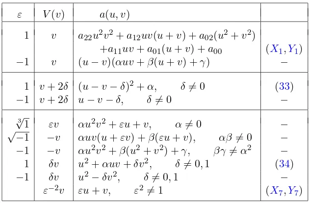
which means that function a possesses some generalized symmetry property. All biquadratic polynomials which satisfy this identity can be found directly. They are listed in the Table1(up to the inversion (u, v)→ (1/u,1/v); the restrictions on the parameters are introduced in order to avoid the intersections and to provide the conditionaauv6=auav). Now we only have to find
the coefficients of f, g, p, q which are quadratic polynomials, in accordance to the Lemma 1. This is done by the direct computations which show that the most cases are empty. As a result, we obtain the pairs (X1,Y1), (X7,Y7) and also the pairs
where a = u2 +αuv +δv2. However, these lattices can be brought to the particular cases of the lattice (X1,Y1) by the transformation (10). For the lattices (33) one should apply the
substitution
u→u+ (β+δ)x+ (γ−δ)y−δ(n−1), v→v+ (β+δ)x+ (γ−δ)y−δn
and the new variables satisfy the lattices (X1,Y1) witha= (u−v)2+α. For (34), the analogous
Table 1. Solutions of the equationεa(u, v)V′(v) =a(V(v), u).
ε V(v) a(u, v)
1 v a22u2v2+a12uv(u+v) +a02(u2+v2)
+a11uv+a01(u+v) +a00 (X1,Y1)
−1 v (u−v)(αuv+β(u+v) +γ) −
1 v+ 2δ (u−v−δ)2+α, δ 6= 0 (33)
−1 v+ 2δ u−v−δ, δ6= 0 −
3
√
1 εv αu2v2+εu+v, α6= 0 −
√
−1 −v αuv(u+εv) +β(εu+v), αβ6= 0 − −1 −v αu2v2+β(u2+v2) +γ, βγ6=α2 −
1 δv u2+αuv+δv2, δ 6= 0,1 (34)
−1 δv u2−δv2, δ6= 0,1 −
ε−2
v εu+v, ε2 6= 1 (X7,Y7)
2) Let the lattices be of the form (27), (30),h= (v−u1)−2,r =U′V1′. Then
a(u, v) =
2
X
i,j=0
aijuivj =
A11U V +A10U +A01V +A00
U′V′ ,
b(u, u1) =−a(u, u1) =
εA11U U1+εA01U−p1(U1)
U′
U′
1
,
c(v, v1) =−εa(v, v1) =
A11V V1+A10V1+q1(V)
V′V′
1
.
As in the previous case, the first equation implies that functionsU, V are linear-fractional. The other two equations are equivalent to relations
A11V(v) +A10
V′
(v) =−ε
A11U(v) +A01
U′
(v) , (35)
p1(U(u))
U′
(u) =
A01V(u) +A00
V′
(u) ,
q1(V(v))
V′
(v) =−ε
A10U(v) +A00
U′
(v) . (36)
We assume, without loss of generality, that either A=U V + 1 or A=εU−V. Equation (35) implies U(u) = cV(u)−ε
(and, consequently, ε= ±1) in the first case, or U(u) = V(u) +c in the second one. The appropriate substitutions, the M¨obius one in the lattice (27) and the linear one in (30), reduce the problem to the following cases:
ε= 1, U =u, V =v−1, a=−v(u+δv), A=U V +δ, δ 6= 0;
ε=−1, U =u, V =v, a=A=uv+ 1;
U =u, V =v, a=A=εu−v+δ.
Moreover, the functionsp1, q1 are defined from the relations (36) and functionsf(u),g(v),p(u),
q(V) from the equations
f′′= 0, ((V′g)′/V′)′= 0, p′′′ = 0, (q/V′)vv = 0,
in accordance to the Lemma 1. In the first case, after defining the coefficients by the direct computation and the substitutionsu→eu,v→ev and (10) we obtain the lattices (X
second case turns out to be empty and the third one contains, atε= 1, the pair (X2,Y2), up to
the admissible transformations.
3) Let the lattices be of the form (26), (30), h = 1 and r = U′
V′
1. The comparison of the
expressions for the function abrings to the equation
(a11uv+a10u+a01v+a00)U
′
V′ =A11U V +A10U +A01V +A00.
Computing aauv−auav one obtains the relation
(a11a00−a10a01)U
′
V′=A11A00−A10A01
which implies U′′
=V′′
= 0. Therefore, we may assume, after the linear substitutions, U =u,
V =v,A=a. Lemma1says that the right hand sides of both lattices are linear in any variable. Several equations for the coefficients follow from the relations for the functions b,c:
b(u, u1) =a11uu1+a01u1+f1(u) =εa11uu1+εa01u−p1(u1),
c(v, v1) =εa11vv1+εa10v−g1(v1) =a11vv1+a10v1+q1(v).
After the final check of the compatibility condition we arrive to the pair (X4,Y4).
In order to finish the classification we have to consider the lattices with the functionaof the form a(u, v) =a1(u)a2(v).
Proposition 5. The consistent lattices with the condition aauv = auav, are brought by the admissible substitutions to one of the pairs (X5,Y5), (X6,Y6) or (X8,Y8).
Proof . The substitution (7) allows to reduce the problem (temporarily) to the case a = 1. Then the compatibility conditions for the systems (13)–(16) are
hv
h =bu1+b hu1
h , ε hu1
h =cv+c hv
h , ε rv1
r =bu+b ru
r ,
ru
r =cv1+c rv1
r . (37)
As a corollary, the equations hold
bu(logh)vu1 = 0, cv1(logh)vu1 = 0, bu1(logr)uv1 = 0, cv(logr)uv1 = 0.
We will use also the following consequences of the relations (22), (23):
Pu+Qv+k1= 0, Fu+Gv+k2 = 0. (38)
1) At first, assume that both quantities (logh)vu1 and (logr)uv1 do not vanish. Thenb,care
constants andbc=ε. A scaling ofu andv allows to set b=−1,c=−ε. One obtains, after the integration of the equations (13)–(16) and taking (38) into account, the lattices of the form
ux=f(v−u1) +α1u+α, vx =εf(v−1−u) +β1v,
uy =p(εu−1−v) +γ1u+γ, vy =p(εu−v1) +δ1v.
The direct computation proves (notice that f′′
p′′
6
= 0 by assumption) that the linear terms are zero and brings to the pair (X8,Y8).
2) Now let either (logh)vu1 = 0 or (logr)uv1 = 0. Taking the symmetry (9) into account, we
assume for definiteness thath=m(u1)n(v). Then the two first equations (37) take the form
n′
n =bu1 +b m′
m, ε m′
m =cv+c n′
whence
m′
=µm, n′
=νn, bu1 =ν−µb, cv =εµ−νc.
Here we have to consider several subcases.
2.1) Letµν6= 0. After scaling, assume µ= 1, ν=−1, h=eu1−v
. Then
b=e−u1m¯(u)
−1, c=evn¯(v1)−ε,
and two last equations (37) are reduced to relations
¯
m′(u)r+ ¯m(u)ru= 0, ¯n
′
(v1)r+ ¯n(v1)rv1 = 0, ru+εrv1 = 0.
If ¯m= ¯n= 0 then we obtain the lattice of the form (X8,Y8). Otherwise,
b=βe−δεu−u1 −1, c=γev+δv1 −ε, r=λeδ(εu−v1),
where at least one of the coefficients β,γ is not zero. The solution of equations (13), (14) is
F =eu1−v
−βe−δεu−v+f(u), G=εeu−v−1
−γeu+δv +g(v).
The functions P, Q are easily found as well. One easily proves, by use of (38), that δ = −1,
ε = 1, β = γ and the functions f, g are linear. After the direct computation of the constants and the substitution eu →u,e−v
→v (of course, it spoils the gaugea= 1) we come to the pair (X5,Y5).
2.2) Letµ= 0,ν 6= 0. Taking ν = 1,h=ev we obtain
b=u1+ ¯m(u), c=e−vn¯(v1),
ru= 0, ¯n
′
(v1)r+ ¯n(v1)rv1 = 0, εrv1 = ¯m
′
(u)r.
From here, b=u1+εδu+β,c=γe−v−δv1,r =λeδv1 and the solution of equations (13), (14) is
F = (u1+δεu+β)ev+f(u), G=−εev−1 −γue−δv+g(v).
The second equation (38) now reads δεev +f′
(u) +γδue−δv
+g′
(v) +k2 = 0. Since γ 6= 0 in
virtue of the nondegeneracy condition (3), hence δ = 0. Taking r = 1 and solving equations (15), (16) one obtains
P =−εu−1−(u+β)v+p(u), Q=v1+γue −v
+q(v).
However, then the first equation (38) implies γ = 0. Therefore, this case is empty (as well as the case µ6= 0, ν = 0, due to the symmetry (8)).
2.3) Finally, let µ = ν = 0. Then b = b(u), c = c(v1) and one can take h = 1. Then
F =u1+b(u)v+f(u), G=−εv−1−c(v)u−g(v) and substitution into (38) yields
b′
(u)v+f′
(u)−c′
(v)u−g′
(v) +k2 = 0.
From here,
b(u) =αu2+ 2β1u+β, c(v) =αv2+ 2γ1v+γ.
Moreover, elimination of r from the equations (37) brings to the relation
Denote ∆b =b′2−2bb′′= 4(β12−αβ), and analogously forc, then this relation takes the form
2εα+ (∆b+ 2αb)c= 2ε2α+ε(∆c+ 2αc)b.
If α 6= 0 then it follows that ε = 1 and ∆b = ∆c = 0, that is b and c are full squares. The
linear change of variables brings them to the form b = u2, c = v21. Then one finds from (37) that r = (uv1−1)−2 and solution of the equations (15), (16) is P = u−1/(u−1v−1) +p(u),
Q =−v1/(uv1 −1) +q(v). Equations (38) say that functions f, g, p, q are linear and after the
direct computation of the constants we obtain the pair (X6,Y6).
Ifα = 0 thenβ1γ1= 0,β12γ =εγ12β. Since functionsb, c do not vanish in virtue of (3), hence
β1 = γ1 = 0, that is the lattice (1) is linear. Direct calculations prove that either the second
lattice is linear as well, or we arrive to a particular case of the pair (X8,Y8).
4
Associated equations
4.1 Hyperbolic PDE systems
In accordance to the nondegeneracy conditions the equations (1), (2) can be solved with respect to the variablesu±1,v±1:
u1= ˜F(ux, u, v), v−1 = ˜G(u, v, vx),
u−1 = ˜P(uy, u, v), v1 = ˜Q(u, v, vy).
Therefore, these variables can be eliminated from the expressions for the mixed derivatives and some system of partial differential equations appears. The original lattices define its B¨acklund auto-transformation. The form of the system is given by equations
uxy =f4uxuy+f3ux+f2uy+f1, vxy =g4vxvy+g3vx+g2vy+g1,
where the coefficients depend on u,v. Indeed, consider the equalities
uxy =Fu1T(P) +Fuuy+Fvvy =Pu−1T
−1
(F) +Puux+Pvvx.
In the first one the variables u1, v1 should be eliminated only and we see that the expression
for uxy does not depend on vx and is linear inuy. Analogously, elimination of u−1, v−1 in the
second equality proves that the expression for uxy does not depend on vy and is linear in ux.
The formula for vxy is proved analogously.
Proposition 6. In virtue of the lattices from the list 7.1, the variablesu,vsatisfy the respective systems from the list 7.2.
4.2 Ruijsenaars–Toda lattices
As we have already explained in the Introduction, elimination of the variablevallows to rewrite the lattice (1) in the form of Ruijsenaars–Toda type lattice (4), and its symmetry (2) in the form (5). Moreover, the equation (6) is fulfilled as well. The triples of the lattices corresponding to the list 7.1are enumerated in the list 7.3. The remarkable property is that elimination of u
instead of v brings to the same equations. This can be proved without calculations since it is easy to see that the lattices from the list 7.1are invariant with respect to the involution
and the lattices from the list 7.3are invariant with respect to the involution
un↔σu−n, x→ −x, y→ −y,
where σ = 1 for (X1), (Y1), (R1) and σ = −1 in other cases. It should be noted that this
property is not invariant under the general substitutions (7). For an arbitrary choice of the variables u and v the corresponding Ruijsenaars–Toda lattices coincide after a suitable point substitution. As to the lattices (X7), (Y7), (X8), (Y8), they possess the above symmetry only if ε= 1.
4.3 Discrete Toda lattices
Coincidence of the lattices (4) for the variables u and v allows to expand the equations on the square grid and leads to the discrete Toda lattices. More precisely, this property means that the equations (1), (2) define the B¨acklund auto-transformations for the lattices (4), (6) correspondingly. This allows to introduce the variableu(n, m, x, y), so that the pair (u(n), v(n)) is identified with (u(n, m), u(n, m+ 1)) at arbitrary m. Let us rewrite the lattices from the list 7.1denoting the shifts by the double subscripts:
ux=F(u0,1, u, u1,0) =G(u−1,0, u, u0,−1), (39)
uy =P(u0,−1, u, u1,0) =Q(u−1,0, u, u0,1). (40)
Then the following properties are valid:
1) equations F = G and P = Q are equivalent and can be rewritten as the discrete Toda lattice
f(u0,1, u) + ˜f(u0,−1, u) =g(u1,0, u) + ˜g(u−1,0, u); (41)
2) equation (41) is consistent with the dynamics on x andy, that is, the equations obtained by differentiating of this equation in virtue of (39) or (40) are its consequences;
3) the variablesu(n) =u(m, n) for any m satisfy the Ruijsenaars–Toda lattices (4), (6); 4) the variables u(m) =u(m, n) for any n satisfy the analogous lattices (possibly, with the different right hand sides);
5) the variables along the diagonals u(n) = u(m −n, n) satisfy a Toda type lattice with respect to thex-derivatives
uxx= ˜A(ux, u1, u, u−1),
and the variables along the complementary diagonals u(n) = u(m+n, n) satisfy a Toda type lattice with respect to the y-derivatives
uyy= ˜C(uy, u1, u, u−1).
6) all these equations are Lagrangian.
5
Non-Hamiltonian lattices
The pairs (X7,Y7) and (X8,Y8) are of interest as counter-examples to the statement that existence
of one symmetry implies the existence of the whole hierarchy. These lattices do not possess the higher symmetries at arbitrary f,g and ε. In particular, the necessary integrability conditions fail for the associated lattices of the form (4). In accordance to [13] the simplest of these conditions reads
The direct computation proves that elimination of v from equations (X7) brings to the lattice
uxx=
(ux+ 1)(εux−1)
1 +ε
u1,x+ 1 u1+εu −
εu−1,x−1
u+εu−1
and the above condition is fulfilled for this lattice only ifε= 1.
It turns out, however, that the nature of these counter-examples is not too profound. It is easy to see that the non-invertible substitution U = v−u1, V = εu−v1 reduces the lattices
(X8,Y8) to the disjoint pairs
Ux =εf(U−1)−f(U1), Uy = 0; Vx= 0, Vy =εp(V−1)−p(V1).
Analogous, but not so evident substitution exists for the pair (X7,Y7) as well: the variables
U = (1 +ε)(u+v) (εv−1−u)(εv−u1)
, V = (1 +ε)(u+v) (εu−1−v)(εu−v1)
(42)
satisfy the equations
Ux =U(U1+U−ε(U+U−1)), Uy = 0;
Vx= 0, Vy =−V(V1+V −ε(V +V−1)). (43)
In both cases the quantitiesU(n) are the local first integrals for one lattice in the pair, andV(n) for another one. In these variables the consistency of x- and y-flows become trivial and is not related to integrability (although at ε = 1 and for some f, p equations may “accidentally” coincide with integrable Volterra type lattices [23]).
The fact that the local first integrals satisfy the closed lattice with respect to the second independent variable can be easily explained in the framework of the associated hyperbolic system. For the pair (X7,Y7) it is of the form
uxy =
(ux+ 1)(uy+ 1)
u+v , vxy =
(vx−1)(vy−1)
u+v (44)
(notice that the units may be dropped, due to the substitution u → u−x −y, v → v +
x +y, however this leads to nonautonomous lattices). This is the Liouville equation type system [20, 21, 22]. Elimination of the shifts in the first integrals (42) leads to the invariants of this system, that is, to the quantities I(u, v, ux, vx, . . .), J(u, v, uy, vy, . . .) which satisfy the
propertiesIy = 0, Jx= 0 in virtue of (44). It can be proved that, in the case of the hyperbolic
system of the second order, all solutions of the equation Iy = 0 are expressed through the x
-derivatives of at most two basic invariants. Therefore, the invariantsU1,U,U−1must be related
by some differential constraint, as the first equation (5) shows. Finally, notice that the system (44) implies
(loguxy)xy = 0, (logvxy)xy = 0.
This gives the formula for the general solution
u=a(x)b(y) +c(x) +d(y), v =−u+(ux+ 1)(uy+ 1)
uxy
under assumptiona′
b′
6
= 0, and this ansatz reduces the lattices (X7,Y7) to the recurrent relations
a1= εc
′
−1
a′ , c1 =aa1−εc; b1=
d′
+ 1
b′ , d1 =ε(bb1−d).
These relations are equivalent to some Volterra type lattice, for example the substitutiona→εna
and scaling ofx brings to the equation (known to be integrable at ε= 1 [23])
εnan,x =
1
an+1−an−1
6
Concluding remarks
The integrable lattices of the form (1) or (4) admit the very important generalization: their right hand sides may contain parameters which depend onnand define the discrete spectra added by the iterated B¨acklund transformations. Such generalizations are known, actually, for all lattices from the above lists, see e.g. [12,7]. It turns out, however, thatn-dependent lattices (1)are not
consistent with the symmetries of the form (2), only with the higher symmetries of NLS type. The nature of this phenomena is not well understood for the present. It takes place in another situations as well, for example, the dressing chainvn,x+vn+1,x= (vn−vn+1)2+αnis consistent
Another sort of the nonautonomous generalizations is related to the master-symmetries of the lattices (1), (2), see [14,25].
The multifield lattices also should be mentioned. Probably, the earliest example of such kind was found in [26,27]. It generalizes the pair (X6,Y6) in the rational form:
The vectorsu, v satisfy, in virtue of these equations, the system
uxy =hu, viuy+ (huy, vi −1)u, vxy =−hu, vivy−(hu, vyi+ 1)v.
However, an analog of the lattice (R6) is absent in this example.
7
Lists
7.1 Consistent pairs of the Hamiltonian lattices
This research was supported by the RFBR grant # 04-01-00403.
[1] Ruijsenaars S.N.M., Relativistic Toda system, Preprint Stichting Centre for Mathematics and Computer Sciences, Amsterdam, 1986.
[2] Ruijsenaars S.N.M., Relativistic Toda systems,Comm. Math. Phys., 1990, V.133, 217–247.
[3] Bruschi M., Ragnisco O., On a new integrable Hamiltonian system with nearest-neighbour interaction,
Inverse Problems, 1989, V.5, 983–998.
[4] Suris Yu.B., Discrete time generalized Toda lattices: complete integrability and relation with relativistic Toda lattices,Phys. Lett. A, 1990, V.145, 113–119.
[5] Adler V.E., Shabat A.B., On the one class of the Toda chains,Theor. Math. Phys., 1997, V.111, 323–334.
[6] Adler V.E., Shabat A.B., Generalized Legendre transformations,Theor. Math. Phys., 1997, V.112, 935–948. [7] Adler V.E., Shabat A.B., First integrals of the generalized Toda lattices,Theor. Math. Phys., 1998, V.115,
349–358.
[8] Marikhin V.G., Shabat A.B., Integrable lattices,Theor. Math. Phys., 1999, V.118, 217–228.
[9] Adler V.E., Marikhin V.G., Shabat A.B., Canonical B¨acklund transformations and Lagrangian chains,
Theor. Math. Phys., 2001, V.129, 163–183.
[10] Ragnisco O., Santini P.M., A unified algebraic approach to integral and discrete evolution equations,Inverse Problems, 1990, V.6, 441–452.
[11] Shabat A.B., Yamilov R.I., Symmetries of nonlinear lattices,Leningrad Math. J., 1991, V.2, 377–400.
[12] Adler V.E., Yamilov R.I., Explicit auto-transformations of integrable chains,J. Phys. A: Math. Gen., 1994, V.27, 477–492.
[13] Yamilov R.I., Symmetry approach to the classification from the point of view of the differential-difference equations. Theory of transformations, Doctoral Thesis, Ufa, 2000.
[14] Adler V.E., Shabat A.B., Yamilov R.I., Symmetry approach to the integrability problem, Theor. Math. Phys., 2000, V.125, 1603–1661.
[15] Adler V.E., Discretizations of the Landau–Lifshitz equation,Theor. Math. Phys., 2000, V.124, 897–908. [16] Hirota R., Nonlinear partial difference equations. II. Discrete-time Toda equation, J. Phys. Soc. Japan,
1977, V.43, 2074–2078.
[17] Suris Yu.B., Bi-Hamiltonian structure of theqdalgorithm and new discretizations of the Toda lattice,Phys. Lett. A, 1995, V.206, 153–161.
[18] Adler V.E., On the structure of the B¨acklund transformations for the relativistic lattices,J. Nonlinear Math. Phys., 2000, V.7, 34–56,nlin.SI/0001072.
[19] Adler V.E., Suris Yu.B., Q4: Integrable master equation related to an elliptic curve,Internat. Math. Res. Not., 2004, V.47, 2523–2553,nlin.SI/0309030.
[20] Zhiber A.V., Ibragimov N.H., Shabat A.B., Liouville type equations,DAN SSSR, 1979, V.249, 26–29.
[22] Zhiber A.V., Sokolov V.V., Exactly solvable hyperbolic equations of the Liouville type,Uspekhi Mat. Nauk, 2001, V.56, N 1, 63–106.
[23] Yamilov R.I., On classification of discrete evolution equations,Uspekhi Mat. Nauk, 1983, V.38, N 6, 155–156.
[24] Adler V.E., Shabat A.B., Dressing chain for the acoustic spectral problem,Theor. Math. Phys., 2006, V.149, 1324–1337,nlin.SI/0604008.
[25] Nijhoff F., Hone A., Joshi N., On a Schwarzian PDE associated with the KdV hierarchy, Phys. Lett. A, 2000, V.267, 147–156,solv-int/9909026.
[26] Svinolupov S.I., Yamilov R.I., The multi-field Schr¨odinger lattices,Phys. Lett. A, 1991, V.160, 548–552.