Cristian Bartolucci is an assistant professor of economics at Collegio Carlo Alberto. The author is specially grateful to Manuel Arellano for his guidance and constant encouragement. He would also like to thank Stéphane Bonhomme, Christian Bontemps, Raquel Carrasco, Zvi Eckstein, Chris Flinn, Andrés Erosa, Pietro Garibaldi, Carlos González- Aguado, José Labeaga, Joan Llull, Claudio Michelacci, Pedro Mira, Enrique Moral- Benito, Diego Puga, Jean- Marc Robin, Nieves Valdez, and seminar participants at Uppsala University, Bank of Canada, Collegio Carlo Alberto, Bank of Italy, Bank of France, PSE, UQAM, CEMFI, University of Tucuman, University College London, ICEEE (2011), European Meeting of the Econometric Society (2009), Cosme Workshop, EC- Squared Conference on Structural Microeconometrics, SEA meetings (2008), and IZA- ESSLE (2008) for very helpful comments. Special thanks is due to Emily Moschini for excellent research assistance and to Nils Drews, Peter Jacobebbinghaus, and Dana Muller at the Institute for Employment Research for invaluable support with the data. The data used can be made available to other researchers from December 2014 through November 2017 from IAB, BA, Postfach, Nuremberg 90327, Germany, subject to federal data protection regulations and the approval of the German Federal Employment Offi ce. The computer code for replication of the results presented in this paper can be obtained from Cristian Bartolucci, Collegio Carlo Alberto, via Real Collegio, 30, Moncalieri TO, 10024, Italy. cristian.bartolucci@carloalberto.org
[Submitted October 2011; accepted November 2012]
ISSN 0022- 166X E- ISSN 1548- 8004 © 2013 by the Board of Regents of the University of Wisconsin System
T H E J O U R N A L O F H U M A N R E S O U R C E S • 48 • 4
Gender Wage Gaps Reconsidered
A Structural Approach Using Matched
Employer- Employee Data
Cristian Bartolucci
A B S T R A C T
In this paper, we study the extent to which wage differentials between men and women can be explained by differences in productivity, disparities in friction patterns, segregation, and wage discrimination. For this purpose, we propose an equilibrium search model that features rent- splitting, on- the- job search, and two- sided heterogeneity in productivity. The model is estimated using German matched employer- employee data. Overall, the results reveal that female workers are less productive and more mobile than males. In addition, female workers have on average slightly lower bargaining power than their male counterparts.
I Introduction
heterogeneity in fi rms and workers. The structural estimation combines group- specifi c productivity measures and the empirical distribution of fi rms’ productivity estimated from fi rm- level data, group- specifi c friction patterns estimated from individual dura-tion data, and individual wages. The model implies a structural wage equadura-tion, which illustrate the precise relationship between wages, worker ability, fi rm productivity, friction patterns, and bargaining power. The wage equation estimated in this paper may be best understood as the structural counterpart of a standard Mincer equation, in-cluding only wage determinants that are relevant from a theoretical point of view. The model allows for counterfactual analysis, such as the decomposition of the observed wage gaps in terms of the differences in productivity and frictions, or segregation and discrimination, taking into account equilibrium effects.
Understanding wage gaps across different demographic groups always has been a central concern in labor economics. Many studies have focused on explaining how much of the unconditional mean wage differential between groups may be under-stood as wage discrimination.1 The standard strategy involves estimating Mincer- type
equations for both groups and then decomposing the difference in mean wages into “explained” and “unexplained” components. The fraction of the gap that cannot be explained by differences in observable characteristics is considered discrimination. This kind of analysis is very informative from a descriptive perspective but the causal interpretation and the nature of discrimination are not clear. The reason is that most of the observable characteristics included in the standard reduced- form wage equations, such as education or experience may be understood as proxies of the true wage deter-minants, such as productivity, outside options, and the rent- splitting rule. Whenever there is a residual difference between groups in some of these wage determinants, the measure of discrimination may be biased. The primary candidate to generate these biases is a between- group difference in productivity that may persist after controlling for education, occupation, age, and tenure.
To deal with this shortcoming, Hellerstein and Neumark (1999) and Hellerstein, Neumark and Troske (1999) exploit newly available matched employer- employee data to calculate a novel indicator for wage discrimination. They estimate the relative mar-ginal products of various worker types, which are then compared with their relative wages. If productivity is the only wage determinant, which is true if there is perfect competition in the labor market, or if there are no signifi cant differences in friction patterns or in the distribution of fi rms faced by both groups, any difference in wages that is not driven by a difference in productivity may be understood as discrimination.
However, comparing wages and productivity may provide an incomplete picture of the problem. For example, wage differentials across groups are often accompanied by unemployment- rate and job- duration differentials. There is a vast expanse of literature estimating differentials in job- fi nding and job- retention rates across groups, directly observing duration in unemployment and employment, or using experiments such as audit studies.2 Although there is agreement in predicting effects of frictions on wages,3
there is scarce empirical evidence as to how much of the wage gap can be accounted for by the differences in the friction patterns. Also, the variation in worker
composi-1. See Blau and Kahn (2003) and Altonji and Blank (1999) for good surveys. 2. See Chapter 4 in Altonji and Black (1999) for a good survey.
The Journal of Human Resources 1000
tion is likely to be correlated with heterogeneity in the production technology, which generates labor market segregation.4
Estimated structural models may provide a complete interpretation of observed wage gaps as a consequence of between- groups differences in every wage determi-nant. Nevertheless, progress in this direction has been slow, primarily due to the
dif-fi culty in separately identifying the impacts of worker productivity differentials and discrimination, solely from worker- level data. The main references are Eckstein and Wolpin (1999) and Bowlus and Eckstein (2002). Both papers are focused on racial discrimination in the United States and deal with this empirical identifi cation problem through structural assumptions. Eckstein and Wolpin (1999) proposed a method based on a two- sided, search- matching model that formally accounts for unobserved hetero-geneity and unobserved offered wages. They argued that differences in the bargaining power parameter (their index of discrimination) are not identifi ed unless some fi rm- side data are available. They compute bounds for discrimination that were ultimately not informative on the estimation sample they worked with. Bowlus and Eckstein (2002) also proposed a search model with heterogeneity in worker productivity but including an appearance- based employer disutility factor. As long as there are fi rms that do not discriminate, they are able to identify between- groups differences in the skill distribution as well as the proportion of discriminatory employers. The fi rst at-tempts to use an equilibrium search model to study gender discrimination were made by Bowlus (1997) and Flabbi (2010). Bowlus only focuses on the effect of gender differences in friction patterns on wage differentials without distinguishing between differences in productivity and discrimination. Flabbi (2010) uses the identifi cation strategy proposed in Bowlus and Eckstein (2002) to additionally disentangle the effect of productivity differentials.5
In this paper, we link two independent branches of the wage- discrimination lit-erature. We propose a natural step in extending the structural estimation literature focused on wage discrimination. The availability of better data enables us to estimate a more complete model,6 using a more transparent identifi cation strategy to measure
differences in productivity and taking into account the effect on wages of labor market segregation. This approach may also be understood as a step forward from the strat-egy proposed by Hellerstein and Neumark (1999), where only productivity gaps were estimated. Here, we provide a more complete interpretation of the observed wage gap, where the productivity gap is only one of the potential determinants of the difference in wages between males and females.
The model builds upon the equilibrium search model, with strategic wage bargain-ing and on- the- job search presented in Cahuc, Postel- Vinay, and Robin (2006). The model consents rent- splitting and, as in Eckstein and Wolpin (1999), we allow for different rent- splitting rules for male and female workers to capture wage
discrimi-4. See Altonji and Blank (1999) and Bayard, Hellerstein, Neumark, and Troske (2003).
5. To have an estimable model with employee- level data, Flabbi (2010) only includes heterogeneity at the match level, not taking segregation into account, and not allowing for on- the- job search. Flabbi does allow for wage bargaining; however, the bargaining power is not estimated.
nation. The model has two sources of heterogeneity. Workers are heterogeneous in terms of productive effi ciency to capture the effect on equilibrium wages of differ-ences across sexes in productivity. Firms technology is also heterogeneous and its distribution is group- specifi c. This feature allows the model to fi t an economy with segregation. Workers do not fi nd jobs instantaneously and, when working, there is a positive probability of losing the current job. The parameters that describe these events are also allowed to be gender- specifi c in order to capture the effect of frictions on the gender wage gap.
We use LIAB, a 1996–2005 matched employer- employee panel data made available by the German Labor Agency.7 This panel provides us with a unique opportunity to
disentangle the different sources of the gender wage gap, because it contains valu-able information on gender, wages and occupations but also because it is a panel that tracks fi rms as opposed to individuals. Tracking fi rms is essential in the estimation of production functions using panel estimation methods. To the best of our knowledge, this paper presents the fi rst structural estimation using matched employer- employee data to study labor market discrimination.8
To have a more homogeneous sample, we only consider fi rms in West Germany. The gender wage gap in this part of Germany is particularly large. According to Blau and Kahn (2000) the gender hourly wage gap in West Germany is 32 percent; placing west Germany in position 6 in a ranking of 22 industrialized countries. Many research-ers are trying to undresearch-erstand the nature of this large earning differential (Lauer 2000; Heinze and Wolf 2010; Antonczyk, Fitzenberger and Sommerfeld 2010).
The empirical analysis initially involves calculating the empirical distribution of
fi rms’ productivity and differences in productivity between men and women. The link-age between worker- level information and fi rm- level data is essential at this stage. From the worker- level data, we recover the composition of the fi rm during each time period. The production function estimation exploits within fi rm variation in worker composition, capital, and output. We estimate group- specifi c productivity parameters and a fi rm- specifi c technology measure. We fi nd large productivity differentials for women and noticeable differences in the distribution of fi rms faced by both kind of workers.
We then analyze group- specifi c friction patterns by survival analysis. We fi nd that women have higher job- creation rates than men, and that females also have higher job- destruction rates than males. Finally, we estimate bargaining power for male and fe-male workers by means of individual wages, gender- specifi c productivity measures for each fi rm, the gender- specifi c distribution of fi rms’ productivity, and gender- specifi c frictions patterns. In spite of the large wage differentials, on average, women are found to have only slightly lower bargaining power than men.
7. This data set is subject to strict confi dentiality restrictions. It is not directly available. After the IAB has approved the research project, The Research Data Center (FDZ) provides on- site use or remote access to ex-ternal researchers. This study uses the Cross- sectional model of the Linked- Employer- Employee Data (LIAB) (Version 1, Years 1996–2005) from the IAB. Data access was provided via on- site use at the Research Data Centre (FDZ) of the German Federal Employment Agency (BA) at the Institute for Employment Research (IAB) and subsequently remote data access.
The Journal of Human Resources 1002
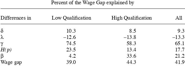
In terms of wages, the raw gender wage gap is 41 percent. It turns out that most of the gap—65 percent—is accounted for by differences in productivity. Differences in destruction rates explain 9 percent while differences in the distribution of the fi rm’s productivity faced by male and female workers explain 17 percent of the total wage- gap. Netting out differences in offer- arrival rates would increase the gap by 13 percent. Presumably, within differences in arrival rates, destruction rates, the distribution of employers and productivity there is some content of discrimination. The economic lit-erature, as well as the legislation of many countries, certainly recognize these potential sources of discrimination. But if we focus our attention on direct wage discrimination, we fi nd that differences in the rent- splitting parameter are responsible for 21 percent of the wage gap, implying that female workers receive wages that are 8.6 percent lower than equivalent males in terms of productivity and treated the same as males in terms of the offer arrival rate, destruction rate and distribution of employers.
The rest of this paper is organized as follows. In the next section, we describe the structural model. Section III describes the data. Section IV presents the estimation of the structural model inputs, namely the productivity measures and friction param-eters. We present and discuss the intermediate results and then describe the empirical strategy used to estimate the structural wage equation and its results. In Section V, the counterfactual experiments are discussed and we compare our empirical results with those found using other strategies for detecting discrimination. Conclusions are offered in Section VI.
II Structural framework
In this section we describe the behavioral model of labor market search with matching and rent- splitting. The primary goal of estimating a structural model is to clearly state a wage- setting equation that enables us to measure the effect of each wage determinant. Once this wage equation is estimated, it becomes straight-forward to obtain the effect of discriminatory wage policies by comparing a man’s wage with the wage that a woman with the same wage determinants would receive. This comparison is equivalent to a standard Oaxaca- Blinder decomposition, the main difference lies in the defi nition of wage determinants. A Oaxaca- Blinder decomposi-tion includes observable characteristics of the worker and the job that are potentially correlated with the wage. By comparison, in our decomposition we include wage determinants that are driven by economic theory. We model the labor market, and therefore we propose a theory that explains how wages are determined. According to that theory, wages are a function of the extent of frictions in the labor market, the productivity of the worker, the productivity of the fi rm and the bargaining power of the worker. Knowing the function that links wages to these wage determinants, we can calculate the portion of the wage gap that is driven by differences in each wage determinant.
of papers. Examples include the previously mentioned papers in the discrimination literature but there are also interesting contributions in measuring returns to education (Eckstein and Wolpin 1995) or in analyzing the effect of a change in the minimum wage (Flinn 2006).
A. Assumptions
We propose a continuous time, infi nite horizon, stationary economy. This economy is populated by infi nitely lived fi rms and workers. All agents are risk- neutral and dis-count future income at the rate ρ > 0.
Workers: We normalize the measure of workers to one. Workers may belong to one of the groups (k) defi ned in terms of gender.9 Workers have different abilities
(ε) measured in terms of effi ciency units they provide per unit of time. The distribu-tion of ability in the populadistribu-tion of workers is exogenous and specifi c to each group, with cumulative distribution function Lk(ε). Group- specifi c distributions of effi ciency units provided by workers are crucial in considering the between- groups differences in productivity. This source of heterogeneity is perfectly observable by every agent in the economy. Each worker may be either unemployed or employed. The workers from a generic group k that are not actually working receive a fl ow utility proportional to their ability, bkε. The workers’ effi ciency in home production is associated with their productivity in the labor market and the parameter that describes that association is allowed to be gender- specifi c.10
Firms: Every fi rm is characterized by its productivity (p). We assume that p is distributed across fi rms according to a given cumulative distribution function Hk(p), which is continuously differentiable with support [pmin,pmax]. The primitive distribu-tion of fi rms’ productivity faced by workers may differ among groups, allowing the model to be robust to labor market segregation. This source of heterogeneity is per-fectly observable by every agent in the economy. The opportunity cost of recruiting a worker is zero.
Each fi rm contacts a worker of a given group k at the same constant rate, regard-less of the fi rm’s bargained wage, its productivity or how many fi lled jobs it has. Unemployed workers receive job offers at a Poisson rate λ0k > 0. Employed workers may also search for a better job while employed and receive job offers at a Poisson rate λ1k > 0 We treat λ0k and λ1k as exogenous parameters specifi c to each group k. Searching while unemployed and searching while employed has no cost. Employment relationships are exogenously destroyed at a constant rate δκ > 0, leaving the worker unemployed and the fi rm with nothing. The marginal product of a match between a worker with ability ε and a fi rm with productivity p is εp.
Whenever an employed worker meets a new fi rm, the worker must choose an em-ployer and then, if she switches emem-ployers, she bargains with the new emem-ployer with no possibility of recalling her old job. If she stays at her old job, nothing happens.
9. The structural model abstracts many dimensions that may be relevant in the wage setting. In order to compare jobs that are as similar as possible, the empirical analysis is clustered at the sector and occupation level. See Section IV for details.
The Journal of Human Resources 1004
Consequently when a worker negotiates with a fi rm, her alternative option is always unemployment. The surplus generated by the match is split in proportions βk and (1 –
βk), for the worker and the fi rm respectively. βk is exogenously given and specifi c to
each group k. We will refer to βk as the rent- splitting parameter. As in Wolpin and Eckstein (1999), we interpret βmale – βfemale as an index of the level of discrimination in the labor market. A difference in β in the same kind of job and sector, reveals differ-ential payments unrelated to productivity and outside options, which are only driven by belonging to a given group.
It is well known that many other factors may have an impact on the rent- splitting parameters. The main candidates are: negotiation skills, risk- aversion, and the dis-count factor. In this model agents are assumed to be risk- neutral and the disdis-count rate is homogeneous across groups. Although this could be part of the story that explains differences in β, there is scant convincing empirical evidence of gender differences in these primitive parameters.11 This could be the reason why risk- aversion and the
discount factor have been held constant across genders in most of the empirical studies on wage discrimination.
It is not clear whether β can be interpreted as a Nash bargaining power. Shimer (2006) argues that in a simple search- matching model with on- the- job search, the standard axiomatic Nash bargaining solution is inapplicable, because the set of fea-sible payoffs is not convex. This nonconvexity arises because an increase in the wage has a direct negative effect over the fi rm’s rents but an indirect positive effect rais-ing the duration of the job. This critique will hold dependrais-ing on the shape of the
fi rm productivity distribution. Whether β can be understood as a Nash Bargaining power is not essential for this study. If this critique holds up, we still interpret β as a rent- splitting parameter that simply states the proportion of the surplus that goes to the worker. A difference in these parameters remains informative about wage- discrimination.
The model assumes that the worker does not have the option of recalling the old employer. Hence, there is no possibility of Bertrand competition between fi rms, as in Cahuc, Postel- Vinay, and Robin (2006). Whether to allow fi rm competition a la Bertrand is controversial. While the Cahuc et al. bargaining scenario may be concep-tually more appealing and may help to avoid the Shimer critique, it is not clear how realistic this assumption is. Mortensen (2003) argues that counteroffers are empirically uncommon. Moscarini (2008) illustrates that, in a model with search effort, fi rms may credibly commit to ignore outside offers to their employees, letting them go without a counteroffer, and suffer the loss, in order to keep in line the other employees’ incen-tives to not search on the job. Moreover, it can be shown that including a marginally positive cost of negotiation, makes it unprofi table for fi rms to try to poach the worker from better fi rms, and then the Bertrand competition vanishes.
In an environment where contracts cannot be written and wages are continuously negotiated, the outside option of the job is always unemployment. In this context, if a worker receives an offer from a fi rm with higher productivity, she must switch. She cannot use this offer to renegotiate with her current fi rm, because she knows that this
offer will not be available tomorrow, and then her future option will be the unemploy-ment.12 This possibility is also discussed in Flinn and Mabli (2010).
Beyond the theoretical relevance of between- fi rms Bertrand competition, this as-sumption is not critical for most of the results presented in this paper. In the Ap-pendix, we illustrate that using the same data with a variation of the model where between- fi rm Bertrand competition is allowed, the gender wage- gap decomposition remains practically unchanged.
This model is similar to the model presented in Flinn and Mabli (2010). The primary difference is in the distributions of productivity. To have a model that is estimable only with employee- level data, they assume that there is a technologically determined discrete distribution of worker- fi rm productivity. In other words, they assume discrete heterogeneity at the match level, while here we assume two- sided continuous hetero-geneity. The model presented here also has the convenient property of producing a closed- form solution for the wage- setting equation.
B. Value Functions
The expected value of income for a worker with ability ε, who belongs to group k, currently employed at wage w(p,ε,k) is denoted by E(w(p,ε,k),ε,k) and it satisfi es:
(1)
ρΕ(w(p,ε,k),ε,k) = w(p,ε,k) + δk[U(ε,k)− Ε(w(p,ε,k),ε,k)] +
λ1k [Ε(w(p,ε,k),ε,k) − Ε(w(p,ε,k),ε,k)] w(p,ε,k)
wmax(p,ε,k)
∫
dF(w(p,ε,k) |ε,k)The expected value of being unemployed for a worker with ability ε, who belongs to group k is given by:
(2) ρU(ε,k) = bkε + λ0k [E(w(p,ε,k),ε,k)−U(ε,k)] wmin(p,ε,k)
wmax(p,ε,k)
∫
dF(w(p,ε,k) |ε,k)Finally, the value of the match with productivity pε for the fi rm when paying a wage w(p,ε,k) to a worker of group k is given by:
ρJ(w(p,ε,k),p,ε,k) = pε −w(p,ε,k) −[δk+λ1kF(w(p,ε,k) |ε,k)]J(w(p,ε,k),p,ε,k),
where F(w(p,ε,k) |ε,k) = 1−F(w(p,ε,k) |ε,k) and F(w(p,ε,k) |ε,k) is the equilib-rium cumulative distribution function of wages paid by fi rms with a productivity lower than p to workers with an ability ε who belong to group k. Note that every parameter is group- specifi c. As the alternative value of the match for the fi rm is always zero, this value does not depend on alternative matches and is therefore independent of the pa-rameters of the other groups of workers. Although every group is sharing the same labor market, all value functions may be considered group- by- group as if they were in independent markets. For simplicity of the notation, we therefore omit the k- index.
The Journal of Human Resources 1006
Note that w(p,ε) is a function of p and ε, therefore given p and ε, the wage is a redun-dant state variable which is only included for exposition simplicity.
These expressions are equivalent to the value functions of the model with hetero-geneous fi rms presented in Shimer (2006), including heterogeneity in workers ability. Here, wages are determined by the following surplus splitting rule:
(3) (1− β)[Ε(w(p,ε),ε)−U(ε)]=βJ(w(p,ε),ε)
After some algebra (see the Online Appendix for the proof13), it can be shown that: w(p,ε) =pε −[ρ+δ+λ1F(w(p,ε|ε)]1− β obtain a fi rst- order differential equation,
w(p,ε) =pε −[ρ+δ+λ1H(p)]1− β
After some algebra, solving for the differential equation yields:
(4) w(p,ε) =pε − ε(1− β)[ρ+δ+λ1H(p)]β [ρ+δ+λ1H(p)]−β pmin
p
∫
dpThis expression states a clear relationship between wages w(p,ε), workers’ ability (ε), fi rm productivity (p), the distribution of fi rms’ productivity (H(.)), friction patterns (λ1,d) and the rent- splitting parameter (β).14 This wage equation is relatively similar
to the one proposed by Cahuc, Postel- Vinay, and Robin (2006) when the wage is bar-gained between a fi rm with productivity p and an unemployed worker with ability ε.15
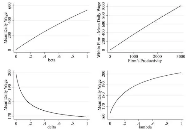
As expected, the model predicts that the mean equilibrium wage increases in β, and that the mean wage paid by a fi rm with productivity p increases in p. Note in Equation 4 that if β=1⇒w(p,ε)= pε, the maximum wage that a fi rm with productivity p can pay to a worker with ability ε is the full productivity. If β=0⇒w(p,ε)= p
minε that is the minimum wage that a worker would accept to leave unemployment. Figure 1 il-lustrates that the mean equilibrium wage increases when λ1 increases and when δ de-creases.16 Many models in the literature predict that the mean equilibrium wage
de-creases in the amount of frictions (see, for example, the models in Burdett and Mortensen 1998, Bontemps, Robin, and van den Berg 2000; Postel- Vinay and Robin 2002; Cahuc, Postel- Vinay, and Robin 2006). Wages are decreasing in the degree of frictions (λ1 / d) due to a compositional effect and a direct effect. The compositional 13. Online Appendix available at http: // sites.google.com / site / cristianbartolucci / DetectingWageDiscirmination _OA.pdf.
14. Solving the differential equation we have:
w(p,ε) =pε − ε(1− β)[ρ+δ+λ1H(p)]
In Section A2 of the Online Appendix, we show that the minimum accepted productivity is independent of the worker type. Therefore we directly write pmin in the lower limit of integration.
15. Note that in Cahuc et al. (2006), when the wage is bargained between a fi rm and an unemployed worker, Bertrand competition does not hold. Therefore, their proposed scenario and ours are equivalent. The only difference stems from the fact that both parts take into account future Bertrand competition.
effect is due to the fact that when frictions decrease the workers are, on average, higher in the job ladder. The direct effect is because the model is asymmetric in workers and employers, when frictions decrease the outside option of the worker increases but the outside option of the fi rm is always zero.17
We assumed that the economy is in a steady state. The standard stationary equilib-rium conditions are exploited. The infl ow must balance the outfl ow for every stock of workers, defi ned in terms of individual ability, employment status, and for those workers who are employed, fi rm productivity.
• The infl ow to unemployment must be equal to its outfl ow, λ0μ=δ(1− μ), where μ is the unemployment rate given by:
(5) μ= δ δ+λ0
• The infl ow to jobs in fi rms with productivity p or lower than p must be equal to its outfl ow:
λ0H(p)μ=[λ1H(p)+δ]G(p)(1− μ)
where G(p) is the fraction of workers employed at a fi rm with productivity p or lower than p. Using Condition 5 and rearranging:
17. See van den Berg and van Vuuren (2010) for a deeper discussion on the effect of friction on wages.
Figure 1
The Journal of Human Resources 1008
(6) G(p)= H(p)
[1+(λ1/δ)H(p)]
This stationary condition, (or its counterpart in terms of wages) is quite com-mon and has been broadly used after Burdett and Mortensen (1998) to infer the primitive distribution of productivity (or the primitive distribution of wages) when only the distribution of productivity (or distribution of wages) for employed workers is observable. Since we use matched employer- employee data, we can directly observe the empirical distribution of productivity at the fi rm level. We use this stationary condition to construct the likelihood for the duration analysis in Section IV.
• The fraction of employed workers with ability ε or lower than ε that are working in fi rms with productivity p or lower than p are (1 – μ)F(ε,p), where F(ε,p) is the joint cdf of ε and p. These workers leave this group due to a better offer, or because they become unemployed; such event occurs with probability
[λ1H(p)+δ]. The infl ow to this group is given by the unemployed workers with ability ε or lower than ε, (that is, L(ε)μ) who receive an offer from a fi rm with productivity p or lower than p. This last event occurs with probability λ0H(p). We now obtain the following condition:
(1− μ)[λ1H(p)+δ]F(ε,p)=λ0H(p)L(ε)μ
Using Conditions 5 and 6 and rearranging: (7) F(ε,p)= H(p)
1+(λ1/δ)H(p)L(ε)=G(p)L(ε)
This expression states that there is no sorting between fi rm’s productivity and worker‘s ability;18 this statement is controversial, and there is an active debate in
the assortative matching literature.
Becker (1973) showed that in a model without search frictions but with transferable utility, if there are supermodular production functions, then any competitive equilib-rium exhibits positive assortative matching. In a more recent work, Shimer and Smith (2000) and Atakan (2006) show that in search models, complementaries in production functions are not suffi cient enough to ensure assortative matching.
After Abowd, Kramarz, and Margolis (1999), the empirical literature has primarily focused on estimating the correlation between worker’s and fi rm’s fi xed effects, us-ing matched employer- employee data. However, there are still no defi nitive results. Abowd et al. (1999) fi nd a negative and small correlation between fi rms and work-ers fi xed effects for France and a zero correlation for the United States. Lindeboom, Mendez, and van den Berg (2010), using a Portuguese matched employer- employee data set, and Bartolucci and Devicienti (2012) fi nd that there is positive assortative matching.
III. Data
A. Linked Employer- Employee Data from the German Federal Employment Agency (LIAB).
We use the linked employer- employee data set of the IAB (denoted LIAB), covering the period of 1996–2005. LIAB was created by matching the data of the IAB establish-ment panel and the process- produced data of the Federal Employestablish-ment Services (social security records). The distinctive feature of this data is the combination of information about individuals with details concerning the fi rms in which these people work. The workers source contains valuable data on age, sex, nationality, daily wage (censored at the upper earnings limit for social security contributions),19 schooling / training, the
es-tablishment number and occupation. Occupation is recorder using a three- digit code but in this paper is collapsed into two categories: high- and low- qualifi cation occupations.20
The fi rm- level data come form IAB Establishment Panel. These data are drawn from a stratifi ed sample of the plants, where the strata are defi ned over industries and plant sizes (large plants are oversampled), but the sampling within each cell is random. The
fi rm’s data provide details on total sales, value added, investment, depreciation,21
num-ber of workers, and sector.22 In particular, only
fi rms with more than ten workers, a positive output and positive depreciated capital were included in our subsample. Since
fi rms of different sectors do not share the same market, we construct separate samples for each sector. LIAB has a very detailed industry classifi cation. We focus on four primary industries: Manufacturing, Construction, Trade, and Services.23 Participation
of establishments is voluntary but the response rates are high (exceeding 70 percent). However, the response rate on some variables key for our purposes is lower. Among survey respondents, only 60 percent of fi rms in the previous four industries provided valid responses for output. To estimate productivity, we need data on output and num-ber of workers in each category. We only consider observations from the old Federal Republic of Germany (West Germany). The fi nal number of observations in our sample of fi rms is 15,174. Table 1 provides descriptive statistics of the fi nal sample of the fi rms.
One of the main advantages of this data set is that it has information for all employ-ees subject to social security in each fi rm.24 The employee data are matched to fi rms
19. In the sample of fi rms used in this paper, 14.7 percent of the worker observations have censored informa-tion on wages. This proporinforma-tion varies signifi cantly across genders and occupations. 4.7 percent of female observations and 18.1 percent of males observations are censored. The proportion of worker observations in high- qualifi cation occupations, with wages that exceed the upper earning limit for social security contribu-tions, is 37.0 percent while the corresponding proportion of low- qualifi cation occupations is 3.1 percent. 20. We assigned the following groups to the low- qualifi cation occupations: agrarian occupations, manual occupations, services and simple commercial or administrative occupations. We classifi ed the following as high- qualifi cation occupations: engineers, professional or semiprofessional occupations, qualifi ed commer-cial or administrative occupations, and managerial occupations.
21. The survey gives information about investment made to replace depreciated capital. 22. For a more detailed description of this data set, see Alda et al. (2005).
The Journal of Human Resources
1010
Table 1
Firms—Descriptive Statistics
Number of Firms
Output (Mean)A
Number of Workers
Women (%) Men (%)
Low Qualifi cation
High Qualifi cation
Low Qualifi cation
High Qualifi cation
Manufacturing 7,354 151.0 4,297,762 11.9 8.1 55.3 24.7
Construction 1,491 30.2 170,786 12.9 11.5 58.1 17.6
Trade 2,078 67.4 247,884 30.6 17.5 34.4 17.6
Services 4,251 30.4 1,043,678 21.1 21.0 38.9 20.0
Total 15,174 92.8 5,760,110 14.2 11.0 51.5 23.4
for which we have valid estimates of productivity through a unique fi rm identifi er. The raw data contains 21,246,022 observations between 1996 and 2005. After the fi nal trimming we have a ten- year unbalanced panel, including a total of 5,760,110 workers’ observations distributed into 15,174 fi rms’ observations.
Given this selection on top of the original oversampling of large plants, the sample becomes less representative. According to the Federal Statistical Offi ce (Statistisches Bundesamt Deutschland), between 1996 and 2005, the proportion of the work force in the manufacturing sector ranges between 25.6 and 31.7 percent. In the sample used in this paper, this proportion exceeds 74 percent (Table 1). For that reason, the analysis is performed clustering at the industry and occupation level and when making infer-ence on the total population, the between- clusters aggregation of results are calculated using weights obtained from the G- SOEP.25
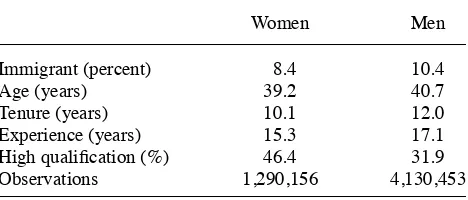
In the sample, women are, on average, younger than men. They also have less ten-ure and less experience. Women are overrepresented in high- qualifi cation occupations. The proportion of immigrants is larger within the male group. See Table 2 for details on the sample of workers.
The primary goal of this study is to understand the gender wage gap. In LIAB, individual wages are top- coded. Consequently, the wage gap is estimated by maxi-mum likelihood assuming that log- wages are normally distributed within the fi rm. The mean of the log- wage for each group is estimated using worker- level data, maximizing saturated normal- likelihoods at the fi rm level. This is consistent with the model if we assume that, conditioning on the worker group, the ability is log- normally distributed.
of employment are not considered liable to social security: civil servants, self- employed persons, unpaid family workers and so- called “marginal” part- time workers (A “marginal” part- time worker is a person who is either only employed for a short- term or paid a maximum wage of €400 per month).
25. The weights for each groups are estimated with the relative frequencies in the 1996–2005 sample of the G- SOEP; these include manufacturing—high- qualifi cation men 12.3 percent; manufacturing—low- qualifi cation men 15.6 percent; manufacturing—high- qualifi cation women 6.1 percent; manufacturing—low- qualifi cation women 4.8 percent; construction—high- qualifi cation men 4.1 percent; construction—low- qualifi cation men 7.0 percent; construction—high- qualifi cation- women 1.1 percent; construction—low- qualifi cation women 0.2 percent; trade—high qualifi cation- men 6.1 percent; trade—low- qualifi cation men 2.9 percent; trade—high- qualifi cation- women 10.5 percent; trade—low- qualifi cation women 2.8 percent; services—high- qualifi cation- men 10.3 percent; services—low- qualifi cation men 4.2 percent; services—high- qualifi cation- women 8.7 percent; and services—low- qualifi cation women 3.1 percent.
Table 2
Workers—Descriptive Statistics
Women Men
Immigrant (percent) 8.4 10.4
Age (years) 39.2 40.7
Tenure (years) 10.1 12.0
Experience (years) 15.3 17.1
High qualifi cation (%) 46.4 31.9
The Journal of Human Resources 1012
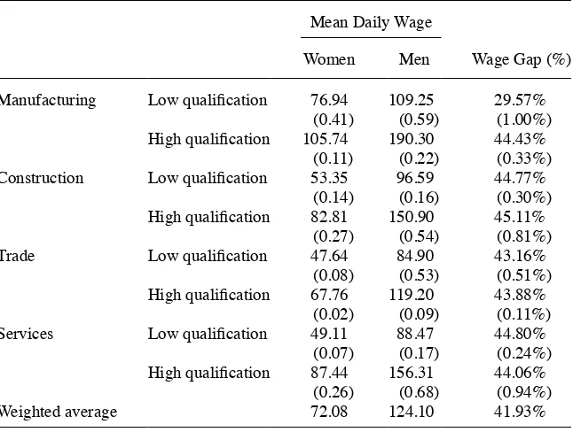
The difference in conditional means is 21 percent (see Table 17 in the Appendix). This implies that women, on average, have salaries that are 21 percent lower than men with the same set of observable characteristics. The unconditional wage differential is 41 percent but it is not stable across sectors and occupations (see Table 3). Mean wages, estimated across industries and occupations, illustrate that the gap ranges be-tween 30 and 45 percent. Wage gaps are signifi cantly different from zero for every sector and for every group. Earning differentials are larger for highly qualifi ed workers in manufacturing, construction, and trade sectors.
B. German Socio- Economic Panel
The LIAB version used in this paper is a panel of fi rms complemented by worker data. As it does not track workers, it is not possible to distinguish between attrition26
26. There is practically no attrition in a establishment level data. There is attrition in the worker- level data due to changes in the worker’s identifi er and changes across establishments of the same fi rm.
Table 3
Gender Wage Gap
Mean Daily Wage
Women Men Wage Gap (%)
Manufacturing Low qualifi cation 76.94 109.25 29.57%
(0.41) (0.59) (1.00%)
High qualifi cation 105.74 190.30 44.43%
(0.11) (0.22) (0.33%)
Construction Low qualifi cation 53.35 96.59 44.77%
(0.14) (0.16) (0.30%)
High qualifi cation 82.81 150.90 45.11%
(0.27) (0.54) (0.81%)
Trade Low qualifi cation 47.64 84.90 43.16%
(0.08) (0.53) (0.51%)
High qualifi cation 67.76 119.20 43.88%
(0.02) (0.09) (0.11%)
Services Low qualifi cation 49.11 88.47 44.80%
(0.07) (0.17) (0.24%)
High qualifi cation 87.44 156.31 44.06%
(0.26) (0.68) (0.94%)
Weighted average 72.08 124.10 41.93%
and job- termination.27 For that reason we use the G- SOEP (German Socio- Economic
Panel) to estimate the group- specifi c transition parameters.28 The G- SOEP is a
rep-resentative repeated survey of households in Germany. This survey has been carried out annually with the same people and families in Germany since 1984 (note that this study only analyzes the 1996–2005 data).29
IV. Empirical Strategy and Results
The discrete nature of annual data implies a complicated censoring of the continuous- time trajectories generated by the theoretical model. Because of these compli-cations, a potentially effi cient full- information maximum likelihood is not considered as a candidate for the estimation. Instead, we perform a multistep estimation procedure.30
Even though it may be asymptotically ineffi cient, we prefer a step- by- step method. One reason is that transition parameters are better estimated using a standard labor force survey, such as G- SOEP. Another reason is that the consistency of every pa-rameter in full- information maximum likelihood is only guaranteed in the case of the correct specifi cation of the full model. However, we are interested in obtaining pro-ductivity differences and transition parameter estimates that are robust to misspecifi ca-tion in other parts of the model, such as the wage setting mechanism. This facilitates the comparability of the intermediate results with previous reduced- form studies that measure gender differentials in productivity and job- retention rates. Moreover, even in an informal way, models are generally incomplete. Therefore, it seems prudent to use estimators that are as robust to misspecifi cation as possible.
The structural model abstracts many dimensions that may be relevant in the wage setting (for example, amenities or union pressure). These omitted dimensions may be mainly associated with different job types. As can be seen in Tables 1 and 2, there are important differences between men and women in terms of occupation and sector. To compare jobs that are as similar as possible, the empirical analysis is clustered at the sector and occupation level. The model is estimated independently for each of the four sectors. In order to control for occupation, transition and the rent- splitting parameters are estimated independently for both types of jobs, in each sector and gender group. We only control for occupation parametrically when we estimate productivity, because we need to consider the full workforce at each fi rm.31
A. Productivity
We assume, as in the theory laid out in Section II, that the distribution of abilities in worker groups within each fi rm fl uctuates around some fi xed density, say l(ε| p,k).
27. Unless the worker leaves the establishment and moves to another establishment within the panel. 28. Cahuc, Postel- Vinay, and Robin (2006) follow the same strategy for estimating transition parameters with the French Labor Force Survey.
29. See Wagner, Burkhauser, and Behringer (1993) for further details on the G- SOEP.
30. Multistep estimation has been done in many papers. Good examples include Bontemps, Robin, and Van den Berg (2000), Postel- Vinay and Robin (2002), and Cahuc, Postel- Vinay and Robin (2006).
The Journal of Human Resources 1014
According to the model (see Condition 7), there is no assortative matching be-tween workers and fi rms. Therefore, for a given worker group (k), the equilibrium distribution of worker types, conditional on the fi rm type, equals the marginal one: L(ε| p,k) = L(ε| k). The model describes the matching process, and the wage setting, for single- worker fi rms. For the sake of consistency with multi- worker fi rms, we as-sume that workers are perfectly substitutable in the production process, between and within skill categories (k’s). Equivalently to Cahuc, Postel- Vinay, and Robin (2006), we defi ne the total amount of effi cient labor employed at fi rm j at time t as: period output at the constant- return Cobb–Douglas function of capital and quality adjusted labor input. constant return to scale, has already been used in the discrimination literature to esti-mate between- group productivity gaps (for example, Hellerstein and Neumark 1999; Hellerstein, Neumark and Troske 1999). We are primarily interested in four groups of workers depending on gender (men and women) and occupation (high- and low- qualifi cation). We normalize γhm = 1 considering highly qualifi ed male workers as the reference group.32 As such, γ
k=γk/γhm is the proportional productivity of group k
relative to the productivity of highly qualifi ed male workers.
We further assume that fi rms can adjust capital instantaneously, what makes Equa-tion 8 totally consistent with the theory presented in SecEqua-tion II, where we have as-sumed that the productivity of a match is pε. If the fi rm chooses the level of capital, the fi rm solves the following problem:33
max Kjt
(AjK(1jt−α)Lαjt−rKjt)
where r is the cost of capital. Therefore—that is the optimal choice of capital given the stock of workers and the fi rm specifi c productivity parameter —is:
K*jt(Aj,Ljt)=Ljt 1− α
Note that Equation 9 is equivalent to the production function presented in Section
gory, we estimate the production function in logs imposing that the relative difference in productivity between low- and high- qualifi cation occupations is constant across gender (γlw = γlγw). is a zero mean stationary productivity shock.
The model predicts that more productive fi rms are able to attract more workers of every type. Moreover, the optimal choice of capital depends on Aj. As a result, produc-tive inputs are correlated with the fi rm fi xed effect (that is cov(Aj,Ljt)≠0 and
cov(A
j,Kjt)≠0 ), which would generates inconsistent estimates of α and γ if we used
ordinary least squares in the estimation. Therefore, we estimate Equation 10 by within- fi rms nonlinear least squares to remove the fi rm fi xed effects.
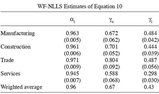
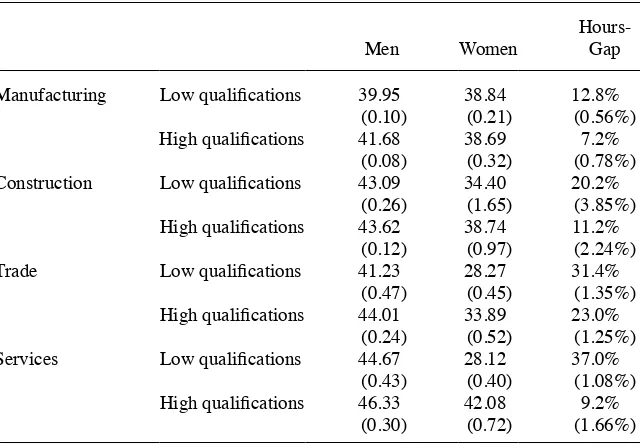
The within- fi rms nonlinear least squares results are presented in Table 4. Women’s productivity is lower than men’s productivity in similar jobs. This difference ranges from 20 to 41 percent. On average across sectors, female workers are 33 percent less productive than males in each job. One of the primary candidates to explain this large productivity gap, is that these estimates are not taking into account that women work, on average, fewer hours than men. Using the G- SOEP36, we fi nd that the average
hour- gap is 19.9 percent, hence, differences in hours are likely to be one of the main determinants of the productivity gap.37
Low- qualifi cation workers are also found to be between 51 percent and 70 per-cent less productive than highly qualifi ed workers. As in most production function estimations using microdata, α is found to be very near one, and hence, the marginal productivity of capital is near zero but statistically different from zero. Although this
fi nding is standard,38 the main results of this paper are not very sensitive to this issue.
If instead of α = 0.96, we include an α more realistic like 0.6; the wage gap decompo-sition does not change signifi cantly.
34. There were problems of convergence in the estimation of Equation 8 using value added. For that reason, output measures where used in the estimation of α and γ in Equation 8. If a constant fraction of output is spent on materials, both estimators are consistent for α and γ. There is only a difference in the constant term of Equation 8.
On the other hand, to estimate pj in Equation 9, the constant term matters, and hence we use measures of value- added.
35. Assuming that a constant fraction (d) of capital depreciates by unit of time:
log(d)+log(Kjt) . Therefore aklog(d) goes to the constant term. 36. LIAB does not provide information on hours.
37. Although differences in hours are illustrated as being important, the primary results of this paper remain valid. We only mention them in order to have a better understanding of the estimated productivity gap. See Section VA for a more detailed discussion of this issue.
38. One interpretation of this result is that Kjtd only captures variable capital whereas fi xed capital is sub-sumed in the fi rm effect. If this is the case, the constant returns restriction is dubious.
The Journal of Human Resources 1016
Pioneered by Hellerstein and Neumark (1999) and Hellerstein, Neumark and Troske (1999), differences in productivity across genders are now well documented in the literature. The fi rst paper fi nds, with Israeli fi rm- level data, a productivity gap of 17 percent. The second paper, using a U.S. sample of manufacturing plants, reports a productivity gap of 15 percent. These studies have been criticized mainly due to the potential endogeneity of the proportion of female workers in the fi rm.39
In this paper, we treat the number of workers of each group as potentially correlated with the fi rm fi xed effect.40 Estimating Equation 10 by within- fi rm non linear least-
squares, the fi rm fi xed effect is completely removed; hence, our estimates are robust to a correlation between the fi rm fi xed effect and the fi rm labor input level but also robust to a correlation between the fi rm fi xed effect and the labor composition of the
fi rm. In this data set, we fi nd a signifi cant correlation between the fi rm’s fi xed effect and the fi rm’s labor input. Estimating Equation 10 by NLLS without fi xed effects, γ’s estimates are signifi cantly lower, the average of γwNLLS across sectors is 0.38 and the
average of γlNLLS across sectors is 0.26. See Table 12 in the Appendix.
The estimates presented in Table 4, require orthogonality of productive inputs to the sequence of shock ujt. In the theory presented in Section II, we abstract from produc-tivity shock. Assuming that ujt is uncorrelated with the productive inputs would be consistent with the model. As we assume that capital is perfectly adjustable, if the productivity shock is observed by the manager after production takes place, capital is exogenous and our results are consistent. Nevertheless, this extra assumption could be
39. See Altonji and Blank (1999).
40. Indeed, the model predicts that more productive fi rms are able to attract more workers of every type. Therefore, the total labor input will be correlated with the fi rm fi xed effect but not with the labor input composition.
Table 4
Production Function Estimates
WF- NLLS Estimates of Equation 10
αl γw γl
Manufacturing 0.963 0.672 0.484
(0.005) (0.062) (0.042)
Construction 0.961 0.701 0.444
(0.006) (0.052) (0.039)
Trade 0.971 0.804 0.487
(0.009) (0.092) (0.056)
Services 0.945 0.588 0.298
(0.007) (0.068) (0.030)
Weighted average 0.96 0.67 0.43
avoided by dropping capital altogether and estimating Equation 9 directly. Results of this last exercise are presented in Table 11 in the Appendix. The estimates of γw and γl are not statistically different from the ones that come out from the estimation of Equa-tion 10, what suggests that the productivity shock is not observed before the manager chooses the level of K. The current productivity shock also might affect the vacancy creation, making it possibly correlated with Ljt∀t>t , which would go against the condition of strict exogeneity required for consistency of fi xed- effects estimators. As in the case of capital, the number of vacancies opened by the fi rm would not be cor-related with the productivity shock if ujt were realized ex- post the production takes place. However, there is large literature suggesting that productive inputs are deter-mined simultaneously with the productivity shock.41 It is possible to estimate α and γ
k
by GMM using internal instruments, assuming that Ljt and Kjt are predetermined. For the sake of robustness of our results, we have explored this possibility but unfortu-nately there is a severe problem of lack of precision on the GMM estimates of the γ parameters (See Section IA in the Appendix for details).
B. Labor Market Dynamics
In the model described is Section II, job terminations might occur endogenously, due to job- to- job transitions, or exogenously, due to job destruction. As both processes are Poisson, the model defi nes the precise distribution of job durations (t) conditional on the fi rm productivity (p):
(11) C(t|p)=[δ+λ1H(p)]e−[δ+λ1H(p)]t
We use the G- SOEP to estimate transition parameters. Unfortunately, this data set does not have productivity measures, so we estimate λ1 and δ treating p as an unob-servable. To do this, we maximize the unconditional likelihood C(t)= ∫C(t|p)g(p)dp, where g(p) is the probability density function of the fi rm’s productivity among em-ployed workers implied by the model.
Taking derivatives with respect to p in Equation 6, we obtain the density of fi rm productivity in the population of workers as:
(12) g(p)= (1+λ1/δ)h(p)
(1+λ1/δ)H(p)
In the Appendix we show the individual contributions to the unconditional likeli-hood become simple enough to be estimated and are given by:
C(t)=δ(1+λ1/δ) λ1/δ
e−x x dx
δt
(1+λ1/δ)δt
∫
Integrating the unobserved productivity out of the conditional likelihood removes p and all reference to the sampling distribution H(p). This method is robust to any misspecifi ca-tion in wage bargaining. The only required property of the structural model is that there exists a scalar fi rm index, in this case p, which monotonously defi nes transitions.
The Journal of Human Resources 1018
In the Appendix42, we show how to obtain the exact form of the likelihood that takes
into account that some durations are right- censored, while others started before the survey’s beginning. Finally, an individual contribution to the log- likelihood is:
ℓ(t
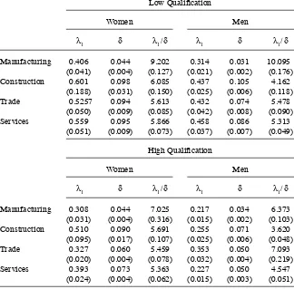
Maximum likelihood estimates are reported in Table 5. The average duration of an employment spell, 1 / δ (possibly changing employers), is between 10 and 32 years but the mean duration across sectors is 20.2 years. The average time between two outside offers, 1 / λ1, ranges from 1.7 to 4.6 years. These results seem to be fairly large but they are compatible with the previous literature. van den Berg and Ridder (2003) used a similar specifi cation but with German aggregated data, and found δ to be equal to 0.060 and λ1 / δ equal to 6.5,44 Here, the weighted average of δ across sectors and
groups is 0.0574 and the weighted average of λ1 / δ is 6.41.
Highly qualifi ed workers have, in general, lower transition rates to unemployment and lower on- the- job offer arrival rates. Women are more mobile than men in terms of job- to- job transitions and, in general, have higher job- destruction rates. Considering
λ1 / δ as an index of friction (van den Berg and Ridder 2003), we do not fi nd signifi cant
differences in the extent of labor market friction between men and women.
C. The Wage Equation: Closing the Model
The structural wage Equation 4 can be written as:
wjti= εiwjtkp (pj,βk,Hk(p),λ1k,δk)
As illustrated in Equation 7, ε is statistically independent of p, thus
42. Online Appendix available at http: // sites.google.com / site / cristianbartolucci / DetectingWageDiscirmination _OA.pdf.
43. The MATA code for computing the exponential integral and the MATA code to maximize this likelihood are available from the author upon request.
44. van den Berg and Ridder (2003, p.237) report monthly rates for λ1 = 0.028 and λ1 / δ = 6.5.
E(w
jti)=E[εiwjtk p (p
j,βk,Hk(p),λ1k,δk)]=Ek(εi)E[wjtk p (p
j,βk,Hk(p),λ1k,δk)]
Ek(εi) = γk is the mean effi ciency units of workers in group k, relative to the male highly qualifi ed group. Therefore, the predicted mean wage for workers of group k working in fi rms with productivity pj at time t is:
(13) E(wjtk)=γkwjtkp (pj,βk,Hk(p),λ1k,δk)
The group chosen for normalization is irrelevant. Changing this group to a generic group k, we would change our measure of productivity. Instead of pj, that is, the pro-ductivity measured in terms of effi ciency units of highly qualifi ed males, we would have pkj =γkpj —that is, the productivity measured in term of effi ciency units of
Table 5
Transition Parameters—Maximum Likelihood Estimates
Low Qualifi cation
Women Men
λ1 δ λ1 / δ λ1 δ λ1 / δ
Manufacturing 0.406 0.044 9.202 0.314 0.031 10.095
(0.041) (0.004) (0.127) (0.021) (0.002) (0.176)
Construction 0.601 0.098 6.085 0.437 0.105 4.162
(0.188) (0.031) (0.150) (0.025) (0.006) (0.118)
Trade 0.5257 0.094 5.613 0.432 0.074 5.478
(0.050) (0.009) (0.085) (0.042) (0.008) (0.090)
Services 0.559 0.095 5.866 0.458 0.086 5.313
(0.051) (0.009) (0.073) (0.037) (0.007) (0.049)
High Qualifi cation
Women Men
λ1 δ λ1 / δ λ1 δ λ1 / δ
Manufacturing 0.308 0.044 7.025 0.217 0.034 6.373
(0.031) (0.004) (0.316) (0.015) (0.002) (0.103)
Construction 0.510 0.090 5.691 0.255 0.071 3.620
(0.095) (0.017) (0.107) (0.025) (0.006) (0.048)
Trade 0.327 0.060 5.459 0.353 0.050 7.093
(0.020) (0.004) (0.078) (0.032) (0.004) (0.219)
Services 0.393 0.073 5.363 0.227 0.050 4.547
(0.024) (0.004) (0.062) (0.015) (0.003) (0.051)
The Journal of Human Resources 1020
group k. To defi ne Equation 13 in terms of the productivity of group k, we only need to put γk inside the expectation operator:
E(wjti)=E[γkpj−(1− βk)[ρ + δk+ λ1kHk(p)]βk ∫ assuming that εi is distributed as a log- normal.46 Under the steady state
assump-tion, and according to the theory presented in Section II, wjtk exhibits stationary fl uc-tuation around the steady state mean wage E(wjtk) paid by fi rm j with productivity pj.
We estimate Equation 14 by weighted nonlinear least squares at the fi rm level, where
γk, δk and λk are parameters estimated in the previous stages, pj is the productivity of fi rm
j, and vjtk is a transitory shock that comes out from within fi rm aggregation. As usual, the discount factor has been set to an annual rate of 5 percent (daily rate of 0.0134 percent).
Standard errors have to take into account that pj, γ, λ1 and δ are estimated in previous stages. To solve this problem, we combine bootstrap for pj and γ with the analytical solution for λ1 and δ. Hence, we obtain standard errors replicating the productivity estimation and the bargaining power estimation in 200 resamples of the LIAB original sample, with replacement but considering the estimated transi-tion parameters as the populatransi-tion parameters. To correct these preliminary standard errors, we add to them the analytical term corresponding to the standard errors of
λ1 and δ reported in Table 5. The analytical correction is straightforward in this
case, because the estimators come from different samples, such that we can omit the term corresponding to the outer product of the scores in the fi rst and second stages.
Consistent standard errors are given by the squared root of:
Var( ˆβ)=Var( ˆβ| ˆλ1, ˆδ)bootstrap+
where Ξ is the objective function in the optimization, which, in this case is the weighted sum of squares and Ξˆxy= ∂(∂Ξˆ /∂x) /∂y. Second derivatives of Ξˆ are obtained numeri-cally.47
46. The within- fi rm distribution of wages of each worker group is the same as the distribution of ability. As wages are linear in ε, to assume log- normality in the distribution of ε implies log- normal wages for each group within the fi rm.
47. The analytical correction ( ˆΞβλ
1Var( ˆλ1) ˆΞβλ1+ ˆ
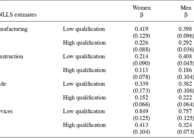
Results are presented in Table 6. Women are found to have lower rent- spitting parameters than men in construction and trade for both high- and low- qualifi cation occupations, and in manufacturing highly qualifi ed occupations. Female workers re-ceive larger portions of the surplus than males in services and in manufacturing low- qualifi cation occupations but these differences are not signifi cant.
There is a clear pattern in terms occupations. Low- qualifi cation workers receive larger shares of the surplus in every sector, considering female and male workers.48
Union coverage, which is higher for low- qualifi cation occupations, and differences in compensating differentials, are potential reasons to explain this difference.
Estimates of the rent- splitting parameter are considerably higher than the param-eters reported in Cahuc, Postel- Vinay, and Robin (2006). This is probably due to the differences in our defi nition of match rents.49 In a similar model estimated with
48. Differences between industries and occupations may be understood as consequence of compensating differentials or differences in union pressure. They cannot be understood as discrimination because we are comparing occupations and not workers.
49. The surplus is defi ned in terms of the productivity of the match and the outside option. Both models imply different outside options. Without Bertrand competition the worker outside option is unemployment. While allowing for Bertrand competition, the worker’s outside option is the whole productivity of the poach-ing fi rm. As the outside option in the model with Bertrand competition dominates the one in the model without Bertrand competition, the estimated bargaining power is smaller.
Table 6
Rent- Splitting Parameter Estimates
WNLLS estimates
Women
β Men β
Manufacturing Low qualifi cation 0.419 0.398
(0.129) (0.096)
High qualifi cation 0.226 0.292
(0.088) (0.036)
Construction Low qualifi cation 0.214 0.408
(0.090) (0.045)
High qualifi cation 0.113 0.186
(0.078) (0.104)
Trade Low qualifi cation 0.339 0.382
(0.173) (0.106)
High qualifi cation 0.152 0.222
(0.066) (0.064)
Services Low qualifi cation 0.849 0.757
(0.125) (0.125)
High qualifi cation 0.413 0.324
(0.104) (0.073)
The Journal of Human Resources 1022
U. S. employee- level data by Flinn and Mabli (2010), the overall bargaining power is found to be 0.45. Here, the weighted average across cells is remarkably similar, 0.421.
Allowing between- fi rms Bertrand competition as in Cahuc, Postel- Vinay, and Robin (2006), changes the magnitude of β for males and females but not the difference across genders. In the Appendix, we present a numerical exercise, where β is recovered by the simulated method of moments using the same data and a model with between- fi rm Bertrand competition. The bargaining power is found to be signifi cantly lower; the weighted average is 0.219 but the gender and occupation patterns do not change. Women are found to have lower bargaining power than males in construction and trade, while there is no clear pattern in manufacturing and services. As in the model without Bertrand competition, workers in low- qualifi cation occupations are also found to have higher β than workers in high- qualifi cation occupations. These fi ndings are not consistent with results found in Cahuc, Postel- Vinay, and Robin (2006), where they
fi nd a positive association between bargaining power and job qualifi cation in France. As in this case we are estimating a similar model to Cahuc, Postel- Vinay, and Robin (2006), this occupation pattern does not seem to be a modeling artifact but instead is a difference between German and French labor markets.50
Differences in rent- splitting parameters are not signifi cant in every sector. We only
fi nd that male workers receive larger shares of the surplus than females in the con-struction sector, where bootstrap p- values of the differences in β are 4.5 percent for low- qualifi cation workers and 9.6 percent for high- qualifi cation workers.
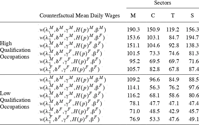
V. Wage-
Gap Decomposition
The structural wage setting equation provides us with a direct way to isolate the effect of each wage determinant on the overall wage differential. Hence, we are able to calculate what fraction of the wage gap is due to segregation or differ-ences in the rent- splitting parameter, productivity, or friction patterns. Although the model takes into account the equilibrium effects of changes in the primitives, this is always conditional to what we have defi ned as primitives. For example, there are good reasons to think that the offer arrival rate might be a function of the distribu-tion of offers and the bargaining power. Changes in the distribudistribu-tion of offers and the bargaining power might change the search effort of the worker but in the model we do not endogeneize wage effort. Moreover, differences in productivity also might be a function of frictions. If a demographic group faces a labor market with more frictions, its members are likely to accommodate their optimal investment in human capital. In principle every mechanism could be endogeneized, and for sure the decomposi-tion would more complete and its interpretadecomposi-tion would be cleaner. The purpose of the estimation presented in this paper is to provide a wage gap decomposition to have a better understanding of the main determinants of wage differentials between male and women. This is not a fi nal answer because we are not explaining what is causing the difference in each wage determinant but our results provide insights of relative importance of each wage determinant in the determination of the wage gap.