9a06c etri manuscript

(1)

3/14/2017 https://etrij.etri.re.kr/etrij/author/Confirmation.do

https://etrij.etri.re.kr/etrij/author/Confirmation.do 1/1

> Paper Status > Submission Information

Submission Information

Article information Authors information

Manuscript Type Regular Paper : RP17030175

Title The Novel PushFront Fibonacci Windows Model for Finding the Emerging Patterns with Better Completeness and Accuracy

Abstract

Mining emerging patterns (EPs) has been wellstudied. Principally, to find EP in streaming transaction data, the streaming is first divided into some timewindows containing a number of transactions; itemsets are generated from transactions in each window and then the emergent of itemsets is evaluated between two windows. In tilted time windows model (TTWM), it is assumed that people need support with finest accuracy from the most recent windows, and accept coarser accuracy from the older windows. Therefore, limited array’s elements are used to keep all support data in a way to condense old windows by merging them inside one element. Capacity of elements in accommodating the windows is modeled using a particular sequence number, where some front elements’ capacity is set to one window in order to serve most accurate support. However, in a stream, as new data come, current element’s updating algorithms create many null elements in array hence data become incomplete. This article proposes the Pushfront TTWM and Pushfront Fibonacci windows model (PFFWin) as solutions. Experimental work shows that PFFWin is able to grab more EPs than existing TTWM based models.

Keywords Data stream mining, Emerging patterns, Fibonacci numbers, Frequent Patterns, Time windows models Research Field ICT Strategy

Self Evaluation

Q) What do you think are the innovative ideas, new results, new applications or new developments of high interest that significantly impact the field?

A) Contributions are novel time windows models: PushFront Tilted Time Windows Model and PushFront Fibonacci Windows Model which improve the accuracy of traditional Tiltedtime windows model, and its derivation models in finding the Emerging Patterns

Resubmission

I. Introduction

Data are being produced and streamed continually in a big volume and high velocity by tremendous number of unusual

sources such as censors and social media in information era [1]. Making sense of these huge data streams is a task that continues to rely heavily on human judgement and therefore, recognizing patterns contained in the streaming becomes a crucial job [2]-[3]. Among the patterns, the emerging patterns (EPs) are one which is worth to mining as they reflect the itemsets’ popularity change from one period of time to another. The problem of mining EP has been well-studied [4]-[7] and EP concept also has been broadly implemented to solve problems in many areas such as to find change in networks [6] and customer behavior in online markets [7].

The streaming can be first divided and loaded into several time-windows to find EP in a streaming data. A window contains several transactions and the itemsets are generated from transactions in each window. An itemset is said emerging from two ordered pair windows W1 to W2 if its support’s growth rate from W1 to W2 satisfies minimum support growth (mingrowth) threshold [4]. A mechanism called tilted-time windows model (TTWM) is proposed to maintain itemsets’ support recorded in all windows [8]. The model assumes that people need supports with finest accuracy only from some recent windows, but they accept coarser accuracy from older windows [9]-[10]. The challenge is how to condense supports data found in a big number of windows inside smaller number of elements of array, i.e. sup[i], in effective and efficient way.

The maximum number of windows that can be merged into array’s elements, or element’s capacity, can be modeled using a certain numbers sequence. Element sup[0] is particularly storing support in currently being processed window, but with a purpose to serve the finest support values, some front elements’ capacities are set to contain only one window. Two

models derived from TTWM: Logarithmic tilted-time

The Novel Push

-

Front Fibonacci Windows Model

for Finding the Emerging Patterns with Better

Completeness and Accuracy

(4)

windows model (LWin) uses geometric-like sequence G = {1; windows being merged inside sup[i], which is either equal to null or F[i]. Sequence of elements’ volume is particularly called the volume sequence.

The main problem of traditional TTWM hence LWin and FWin are the occurrence of null elements even when they should provide the most accurate support. This situation is a big disadvantage in the process to find EP which checks the support’s growth between elements sup[0] and sup[j], j > 0. As a consequence of such data incompleteness, EPs cannot be found at some timestamps hence the trend of pattern’s popularity.

This article, firstly, introduces a novel model, called Push -front Tilted-time Windows Model (PF-TTWM), as the solution for data incompleteness of TTWM. A push-front mechanism is applied to eliminate null, and many front elements can even provide support with finest accuracy. Secondly, this work also proposes a novel Push-front Fibonacci windows model (PF

-Fwin), developed using PF-TTWM’s concept. Fibonacci

sequence F is also used to organize element’s capacity in order N windows can always be accommodated in n–elements array (N ≥ n) by relation given in Eq. (1). However, X.sup[i],vol

∈{1, 2, …, F[i]} in PF-FWin, while in FWin, X.sup[i],vol ∈ {0, F[i]}.

Performance of PF-FWin is compared to FWin and LWin by

processing one million transactions dataset generated using IBM Quest data generator. Process of accommodating the streaming N windows data into n–elements array is modeled using a deterministic finite automaton. Transactions are processed by online streaming method. The new window is created when the number of processed transaction in a window exceeded 10K transactions. The emergent of X is evaluated by inspecting its support stored in X.sup[0] and another X.sup[j], j > 0. X is mined out as EP if X’s support and support growth meet the given thresholds. As the results, number of EP found using PF-FWin, is up to 90% and 275% bigger than using LWin and FWin respectively. These results prove that better

completeness and accuracy offered by PF-FWin can improve

the number of EP found by this model with the runtime performance of PF-FWin is comparable to the other models.

In addition to PF-TTWM and PF-FWin novelties, another contribution of this work is a suggestion about data completeness and accuracy as two main quality characteristics that should be possessed by the models. The rest of article is organized as follows. Section 2 contains review on literatures related to our work. Section 3 defines the proposed solution. Section 4 discusses experimental work and its result, while Section 5 draws the conclusion of this work.

II. Literature Review

Discussion in this section includes the problem of EP mining, TTWM and two state-of-arts windows models derived from TTWM, i.e. Logarithmic TTWM and Fibonacci Windows Model

1. Problem of Mining the Emerging Patterns

The problem of mining EP has been well studied since 1999 [5]-[7], and the implementation of EP in many areas are found in literatures as well. For example, implementation in medical area is found to distinguish similar diseases [12], to classify cancer diagnosis data [13], and for profiling of leukemia patients [14]. In networking environment, EP is implemented to find significant difference in network data stream [6], or for masquerader detection [15].

EP is a class of frequent pattern, where the itemsets are generated using association rule mining. An itemset X is said frequent in dataset D if X’s support the D,

�� X ≥ minsupp , a user-given minimum support threshold [16]. In other words, EP contains related items because their appearance altogether in D is frequent with respect to minsupp.

EP is formally defined as follows [5]. Given an ordered pair of datasets D and D , set I contains all items in both datasets,

(5)

source, but collected at two different time stamps; for example, transactional data of a supermarket, recorded in different months. Alternatively, D and D are also possible from different sources, for example, transactional data from different supermarkets. However, this notion has been adapted to two classes of dynamic datasets accordingly, such as in data stream environment. The examples are to find the change of network by inspecting the IP traffic patterns captured from network routers [6], or to approximate EP from two different class streaming data [7].

EP can also be found in one class of streaming or temporal dataset. In this case, the streaming is divided into several time -windows. Each window contains a number of transactions. EP

is evaluated between two windows W and W , where W

is the most recent window. A method named Dual Support Apriori for Temporal data is proposed to find the emerging trends from temporal dataset using Sliding windows model [4]. But long term itemsets popularity evaluation at multiple time windows cannot be performed because this model only provides two windows: the current and previous one

2. The Tilted-Time Windows Model

TTWM was proposed to store and maintain itemset’s supports from certain number of windows for long term. As explained in [8]-[10], people actually need the most accurate supports only from some recent windows, while coarser accuracy is acceptable from older windows. Therefore, support data in big number of windows should be condensed efficiently into a smaller number of array’s elements.

Technically, each itemset X stores its support data in an n– elements array, denoted as X.sup[i], or sup[i] to simplify. Each sup[i] has a capacity, i.e. maximum number of windows that can be merged inside respective element, while sup [0] particularly stores support in currently being processed window. TTWM models the capacities of sup[i] into a particular numbers sequence i.e. the capacity sequence. The smaller the capacity should create finer accuracy of support. Capacity of some front elements is set to one window to create finest support’s accuracy. The rest elements have different capacities, but the capacity usually sup[i] ≤ sup[i], i< j.

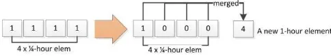
Fig. 1. Elements Updating in Tilted-Time Windows Model

Supposed the transactions are collected and then processed in every ¼-hour, but the manager requires only the most

accurate supports in last one hour processes. As the answer, four elements i.e. sup[0,0,0,0] are initially created to accommodate supports from four windows of ¼-hour data processing respectively. Fig. 1 demonstrates TTWM when updating the elements. After all ¼-hour elements are occupied, or X.sup[1,1,1,1], as support found in current window will be put in sup[0], supports in ¼-hour elements firstly are merged and stored into the 1-hour element. Next, all ¼-hour elements are nullified and sup[0] is now ready to store the current support, or the array becomes sup[1,0,0,0,4] (Fig. 1). This approach can facilitates one day data processing only by 4 (¼ -hour element) + 24 (1-hour elements) = 28 elements, instead of using 4  24 = 96 elements to store all ¼-hour processing results for 24 hours. It is an efficient solution [7]-[9].

3. The Logarithmic Tilted-Time Windows Model

A model derived from TTWM, named Logarithmic TTWM or LWin was firstly introduced in [10] with the goal to store and maintain supports of itemsets for long term. Decision maker got benefit from this approach since time-related query about pattern’s popularity trend can be evaluated, such as patterns that popular once, seasonally popular or everlasting popular. Such benefit cannot be harvested from the other data windows models [9], [10], such as sliding windows [4], [17], [18], damped windows [19], [20] and landmark windows models [21], [22].

LWin is designed to deal the storing results of FP mining in offline data stream. The streaming transactions are divided into N windows, containing uniform number of transactions. The logarithmic approach is proposed to reduce number of elements more significantly, compared to the original TTWM.

N windows can be accommodated in only {1+2_log(N)}

elements. For instance, 1024 windows are fit in only 11 elements, which is very memory-efficient.

LWin uses a sequence, G = {1}∪_{{1[1], 2[2], 4[4], 8[8], so}

on}, to organize the capacity of sup[i] elements, i  0. The right side of union symbol is actually a geometric sequence with ratio r = 2, but aside of each element (called: main element) sup[i], there is an intermediate element, named sub[i] in this article, having the same capacity with its main element i.e. G[i]. Sup[0] has sub[0], but not written here as it is always set to null [7]-[9]. Those articles also explain that the sequence’s ratio is a positive integer and is also changeable in according with the analyst need, although they only explain how LWin works using r = 2. We can see three 1s in sequence G which respectively represents the most accurate support stored in sup[0], sup[1] and sub[1].

(6)

applies the following procedures:

(1) Sup[0] is always filled with the support in current window (2) Sup[1] is filled only by shifting Sup[0] into it

(3) Sub[i] is filled only by shifting Sup[i] into it, while sup[i], i > 1, is filled by sup[i] = sup[i–1] + sub[i–1]; and sub[i–1] is nullified afterward.

(4) The first updating target is a sub[i] = 0, with i is the lowest index, and the updating is continued to its main element sup[i], followed by updating all sup[j] and sub[j], j < i, using procedure number (1), (2) and (3).

(5) When all sup[i] and sub[i] are occupied; increment n = n + 1, and create a new pair elements sup[n] and sub[n] at the back of array. Sup[n] becomes the first updating target, followed by all sup[i] and sub[i], i < n, using procedure (1), (2) and (3).

However, LWin must overcome two situations in its elements’ updating process. If N is exactly �_{, then N} windows are fit to (n+1)-main–elements array. E.g. for N = 8 thus n = 3, eight windows are exactly accommodated in four elements, where the capacity sequence is like {1, 1[], 2[], 4[]}; [] represents an empty sub[i]. However, if N is nearly �_{, then} N windows will be accommodated by (n+1)-main–elements array, plus some intermediate element(s). E.g. for N = 9, thus n

 3, 9 windows will be condensed into 4-elements array plus 1 intermediate element where the formed capacity sequence is like {1, 1, [1], 2, 4}.

Illustration of volume sequence when X if found in N = 1 to 8 windows is given in Fig. 2. Dashed line, bold arrow and thin arrow respectively represent pair of sup[i]-sub[i], first and next done steps. From such illustration, it is known that number of elements hence the memory needed by each itemset is actually maximum 2  {1 + 2log(N)}.

Fig. 2. Volume Sequence and Updating Steps in LWin

4. The Fibonacci Windows Model

FWin or Fibonacci Windows Model was introduced with the goal to improve the memory-efficiency issue occurred in LWin usage, and also to deal with the online data stream mining [11]. The main differences between FWin and LWin is that instead of using “double” geometric sequence, FWin uses Fibonacci sequence, F = {1, 1, 2, 3, 5, so on} to organize elements’ capacity, thus no intermediate element needed in updating process. In addition, distance between capacities in F[i] is smaller than distance in G[i], i>2. According to the principle of TTWM, FWin provides better accuracy than LWin does.

Given n–elements array, sup[i], i = 0 to n–1, elements

updating procedures in FWin are described as follows:

(1) Sup[0] is used to accommodate support in current window

(2) Sup[1] is updated by shifting sup[0] into it

(3) Sup[i], i > 1, is updated by merging sup[i–1] and sup[i–2] into it, or sup[i] = sup[i–1] + sup[i–2]; and then sup[i–1] is nullified afterward. By decrementing i = i – 2, procedure (3) is repeated.

(4) The first updating target is a sup[i] = 0, with i is the lowest index, and the updating is continued to all sup[j], j < i, using procedure number (1), (2) and (3).

(5) When there is no sup[i] = 0 left, increment n = n + 1, so a new element is created at the array’s back, sup[n]. Since sup[n] = 0, it becomes the first updating target by using procedure (4).

Illustration of volume sequence updating when X found in N = 1 to 7 windows is given in Fig. 3. Bold arrow and thin arrow respectively represent first and next done steps.

Fig. 3. Volume sequence and Updating Steps in FWin

Using FWin, N windows can be accommodated in n– elements array, N  n, such as Eq. (1). Value of sup[i].vol is either 0 or F[i]. For instance, 15-elements array can

accommodate 1596 windows. If one window is equal to one

-day data processing, 15-elements array is efficiently fit for 4.37 years data processing, which is also very efficient.

However, both LWin and FWin still possess some shortcomings particularly in data incompleteness issue. Elements sup[1] or sub[1] that should provide the most accurate support, even still possible to be empty. Consequently, queries about support values at several past timestamps cannot be answered. EP in those timestamps also cannot be evaluated hence also the change of itemset’s popularity. Solution on these issues is offered in this work via the proposal about a novel

Push-Front Tilted-Time Windows Model and also its

derivation model, i.e. Push-Front Fibonacci Windows Model

which are explained in next section.

III. The Proposed Methodology

This section explains details of PF-TTWM, followed by the

proposed Push-Front Fibonacci Windows Model. An

automaton for PF-Fwin as updating mechanism is given in this section, and then, EP mining criteria are explained.

(7)

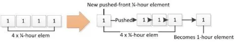
Illustration of the proposed Pushed-front tilted-time windows – PF-FWin – model is given in Fig. 4. The main difference

between PF-TTWM and TTWM is when all elements reached

their respective capacity, PF-TTWM inserts a new element at array’s front, so there is no null element created. In a case given in previous Subsection II-2, the push-front operation makes X.sup = [1,1,1,1] became X.sup = [1,1,1,1,1], instead of X.sup[1,0,0,0,4], such as produced by TTWM. Support in sup[3] becomes sup[4] and represents 1-hour element, while new sup[0] will be filled with new data just arrived.

The main goal of tilting the time-windows in PF-TTWM is still the same as TTWM’s goal, i.e. to reduce memory used to store the supports; but with an improvement to eliminate null elements in PF-TTWM. On the contrary, many front elements’ volumes are filled with 1. Such improvement makes PF -TTWM can provide better data completeness and accuracy, compared to traditional TTWM.

Fig. 4. The Proposed Push-Front Tilted-Time Windows Model

Programmatically, push-front operation is implementable directly in C++ language using pushfront() method. It is a member function of Deque (double-ended queue) container. Amortized time complexity of pushfront() is O(1), which is very efficient, because the element insertion is done at the beginning of the data structure.

2. The Push-Front Fibonacci Windows Model

Notion of PF-TTWM is used to develop PF-FWin with a purpose to improve FWin’s performance to find EP. Using PF -FWin, N windows, in which X is found, can always be accommodated into n–elements array (N ≤ n) by referring Eq. (1), where X. sup[i].vol∈ { , , … , F[i]}.

This approach differs from FWin’s (also LWin’s) approach in term that volume of sup[i] is not only null or F[i] (also G[i] in LWin). Given n–elements array, sup[i], i = 0 to n–1, the complete updating procedures are below:

(1) For i = n–1 to 0, do /*Here, the last element i.e. sup[n–1] becomes the first updating target */

a. Sup[i] += sup[i–1]

b. Shift sup[i–1]  sup[i–2],…,  sup[1]  sup[0] c. Particularly, if i = 0, then Sup[0]  support in current

window.

(2) If volume of sup[n–1] is equal to a Fibonacci element F[n–1] then n = n–1, and procedure (1) is repeated. This

step means that after sup[n–1].vol reached its capacity, then the next updating target is sup[n–2], and so on. (3) If all sup[i].vol reached their capacity, i.e. the volume

sequence = Fibonacci sequence, a new element is pushed at front of array, sup[0], while current array’s indices are all incremented by one accordingly.

Fig. 5 describes the illustration of updating mechanism and

the change of volume sequence in PF-FWin. Bold arrow and

thin arrow respectively represent first and next done steps, where pf-arrow represents the push-front operation and merged-arrow shows the merging process sup[i] += sup[i–1].

Fig. 5. Volume sequence and Updating Steps in PF-FWin

3. The PF-FWin Updating Automaton

PF-FWin’s updating procedures above are modeled in deterministic finite automaton called PFwin Automaton (PFwinA). Formally the automaton is defined as PFwinA(S, I, S0, Z, f), with tuples are explained as follows:

(1) State set S = {Uc: update current element i.e. sup[m], m = n–1, Up: update previous elementi.e sup[m–1], Pf: push front the array}

(2) Input set I = {isFiboSeq, isNotFiboSeq, isFiboElement, isNotFiboElement},

(3) A start state S0 = {Pf}

(4) Stop states set Z = {Uc, Up, Pf}

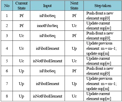
(5) Next-State function f: S  I  S, a function to direct the current state to the next state, after reading the input. Transition table of function f is given in Table 1, while the transition graph is given in Fig. 6. Additionally, Table 1 also lists the step taken after a current state read an input.

PFwinA describes that four conditions may be appearing during the updating process, and they are defined as the input of automaton. First condition is called isFiboSeq. It means the volume sequence generates a Fibonacci sequence or

(8)

The iteration is started by pushing the first element at array’s front, thus PFwinA is started from Pf state, where N = 1, or sup[n–1].vol = 1. The automaton can stop at any state and then it is waiting for the next new window addition.

Fig. 6. PFWin Automaton Graph Transition

Table 1. State Transition Table for PFwin Automaton

No Current _State Input Next _State Step taken

1 Pf isFiboSeq Pf Push_{element sup[0]}-front a new

2 Pf isnotFiboSeq Uc Update current _{element sup[}_m_]

3 Uc isFiboSeq Pf Push_{element sup[0];}-front a new

4 Uc isFiboElement Up Update previous element: m = m–1; update sup[m] 5 Uc isNotFiboElement Uc Update current _{element sup[}_m_]

6 Up isFiboSeq Pf Push_{element sup[0]}-front a new

7 Up isFiboElement Up Update previous element: m = m–1; update sup[m] 8 Up isNotFiboElement Uc Update current _{element sup[}_m_]

To proof that PFwinA can generate volume sequence as defined in Eq. (1) using push-front approach, the following properties are developed and their proofs are given.

Property 1: when Fibonacci sequence has not been developed yet, PFwinA is repeatedly updating sup[m] until sup[m].vol = F[m]. We have to proof that for sS – {Pf}, f(s, isNotFiboElement) = t  t = Uc; Pf is excluded since it represents a state where isFiboSeq is true

Proof: by contradiction, assume sS – {Pf} where f(s, isNotFiboElement) = t  t Uc. By inserting all sS – {Pf} into next-state function above: f({Up, Uc}, isNotFiboElement)

= f(Up,isNotFiboElement)∪f(Uc,isNotFiboElement) = {Uc};

since all function results t=Uc, thus assumption is not correct, therefore Property 1 is correct.

Property 2: After sup[n–1].vol=F[n–1], PFwinA continues to update sup[n–2]. The proof is clearly given in Table 1 that

sS, f(s, isFiboElement) = t  t = Up, which means, PFwinA is updating the previous element i.e. by decrementing m=m–1, and then updating sup[m].

Property 3: the second push-front operation taken after

{sup[i].vol} = a Fibonacci sequence generates sup[n] = F[n], n > 1, i = 0 to n–1.

Proof: supposed volume sequence = a Fibonacci sequence, thus {sup[i].vol} = {1, 1, 2, …., F[n–2], F[n–1]}. The first push-front makes volume sequence = {1}∪{1, 1, 2, .., F[n–2], F[n–1]}. Summation of F[n–1] + F[n–2] creates the next Fibonacci element F[n], and stored in sup[n].

4. Finding EP with PF-FWin

Finding EP over the data stream with PF-FWin (and other

TTWM models) is to cope with big supports as the merging results of some supports. As a consequence, GR(X) formulation and mingrowth become two main keys to affect to the number of EP that can be found from the streaming.

This article evaluates the emergent of X by inspecting X.sup[0], i.e. the current support and another X.sup[j], j > 0. X is said an -EP, > 0, if two following criteria are met:

(1) X is frequent in current window, or X.sup[0] minsupp

(2) GR(X) from sup[j] to sup[0] , where GR(X) is defined in this work as Eq. (3):

GR X =(X. sup[_{X. sup}0] −X. sup_[_j_] [j])

Such GR(X) formula is slightly different from one defined in original work (introduced in Section II), because sup[j], j >1 possibly contains a big support value. Thus GR is defined so that X’s support growth is said significant if it reaches a certain percentage, e.g. 20%.

IV. Experimental Works, Results and Discussions

The experimental works are conducted to evaluate

performance of PF-FWin compared to LWin and FWin to find

EP in online transaction data streaming. EP quantity from three methods becomes performance indicator of experiment. Online streaming means that itemsets are directly generated from each transaction as it arrives. Each generated itemset will also be directly evaluated whether it is an EP or not using criteria explained in previous section, Subsection 4. Therefore, it is also necessary to evaluate runtime performance of each model to organize the array when accommodating supports found in a big number of windows.

Programs of three models are developed using C++ and compiled in Visual Studio Express 2013’s environment. Those programs are individually run on three different PCs but with a same specification i.e. Intel Core i3 CPU @3.30Ghz-3.30GHz,

2GB RAM, under Windows 7 32-Bit. A container in C++’s

(9)

pushfront(), is used to run push-front operation in PF-FWin’s elements updating process.

1. Experimental Design

Dataset of experiment is generated by IBM Quest Data Generator. It contains one million transactions, and 243 items, where one transaction has 3-10 items. New window is created after 10K transactions are processed in a window, thus there are 100 windows that must be organized by each model. Minsupp is set to 100, while mingrowth  = 20%. The other higher

mingrowth values, e.g. 50%, have also been experimented, but number of found EP is not so big, thus it would not be too interesting to be discussed. Nevertheless, another experiment is also performed using the same dataset and thresholds, but a new window is created in every 10 minutes transactions processing.

Not all itemsets are generated from each transaction, but only itemsets with length ≤ 3 items. The reason is actually made based on characteristic of FP, where the longer itemsets usually have smaller support [16]. It means that short itemsets have higher probability to appear frequently hence emerging quickly. In addition, since we perform online data stream, memory resources must not also be wasted by filling it with long itemsets with small possibility to be frequent and emerging in short term.

2. Results and Discussions

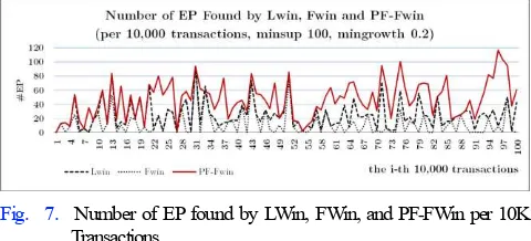
Number of EP found by three models is charted in Fig. 7.

Totally there are 4,708 EPs found by PF-FWin, while FWin

and LWin only found 1,255 and 2,469 EPs respectively. It

means that performance of PF-FWin to find EP is about 1.9

times and 3.75 times or about 90% and 275% higher than LWin and Fwin, respectively.

The runtime performance does not show significant difference between three methods, whereas PF-FWin applies a quite different approach compared to the traditional ones. PF -FWin finished processing all 1M transactions by creating 100 windows in 11H(our):27(M)inutes, while LWin and FWin respectively spent 11H:48M and 11H:28M. Two methods of FWin are faster than LWin. In total, 814,895 different itemsets in 100 windows or about 814.959 itemsets/window/10K transactions are generated.

Compared to two other models, LWin took the longest time to finish all processes because it uses “double” geometric sequence to organize the array’s elements, thus number of elements that must be checked becomes doubled as well. Our observation concluded that the time complexity worst case of LWin is when all or almost all sup[i] and sub[i] are occupied,

or N is almost reaching 2n, such as N = 15. Volume sequence for N = 15 in using LWin is {1, 1[1], 2[2], 4[4]}, and as seen, all sup[i] and sub[i], i> 0, are filled; thus when EP evaluation is

performed, the LWin algorithm must double-check all

elements. As comparison, volume sequence of FWin and PF

-FWin when N = 15 is {1, 1, 2, 3, 0, 8} and {1, 1, 1, 1, 3, 8}

respectively, but number of EP found by LWin, FWin and PF

-FWin when N = 15 is 15, 11 and 66 EP respectively. The number of element in array of all models is actually quite similar. The reason of PF-FWin produces more EP than the other is because the presence of many 1s in front of the array. These instances show that better support’s accuracy of PF -FWin has improved the number of EP that can be found by this model.

Fig. 7. Number of EP found by LWin, FWin, and PF-FWin per 10K Transactions

The worst case of PF-FWIn is occurred when all sup[i].vol reached their capacity, or when volume sequence = a Fibonacci sequence because the array only contains two 1s in its front elements. Fig. 7 shows that LWin outperforms PF-FWin in two windows i.e. N = 7 and 33. If elaborated, PF-FWin’s and FWin reached their capacity, thus the array only has two 1s in its first elements. In contrast, array in LWin has three 1s and it makes more itemsets for the mingrowth. Nevertheless, these instances are good proof that having more 1s in array opens opportunity for the algorithm to find more EP.

(10)

explanation can be gotten by comparing volume sequences when N = 12 and N = 15.

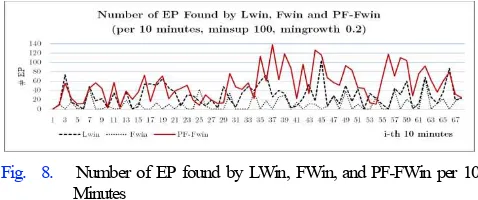
Fig. 8. Number of EP found by LWin, FWin, and PF-FWin per 10 Minutes

On the other side, result from another experiment also quite similar with previous result (Fig. 8). Number of EP found by PF-FWin, FWin and LWin respectively is 3,523, 686 and 1,962 EPs. In this case, FP-FWin also outperforms the other models up to 5.13 and 1.79 times respectively.

First experiment approach shows that as number of transactions in all windows is uniform, the number of itemsets created and number of EP found in each window are constant. However, those numbers are not the same for each window when the second experiment approach is performed. This phenomenon is happened more likely because of two reasons. First, although the timer was set to 10 minutes (or other duration), but the computer results for the time calculation have milliseconds difference. It somehow affects to the number of itemsets generated in each window as well. Second, such itemsets’ difference affects to itemset’s opportunity to be frequent and then emerging in next windows. It also becomes the reason that at certain windows, number of EP found by FWin and LWin is bigger than those found by PF-FWin.

Almost all windows created by both experiment approaches.

However, PF-FWin always outperforms the other two models

to find EP. If we review the GR’s formula, then an itemset X can become an EP only if X.sup[j], hence X.sup[j].vol is not that big. Among of three models, only PF-FWin can meet such requirement because in certain circumstances, many Sup[i].vol contain only one window. Therefore, even if  is made bigger than 0.2, such as 0.5, PF-FWin still becomes the winner.

On the contrary, FWin produces the lowest number of EP, because several elements are empty in some situations. For

example, when N = 14, volume sequence of PF-FWin, FWin

and LWin respectively is {1, 1, 1, 1, 2, 8}, {1, 0, 2, 3, 0, 8} and {1, 1, 2[2], 4[4]}. While LWin has even two 1s in front of the array, FWin only contains one 1; its sup[1].vol is even empty whereas it should provide the most accurate support. Accordingly, very little number of itemsets has opportunity to be frequent and hence emerging in FWin. Adversely, PF-Fwin provides not only better completeness, but also better accuracy since many elements contain only one window.

V. Conclusion

The proposed PF-TTWM and its implementation shows that

PF-FWin has superiority to find more EP and runtime performance in online data stream environment compared to LWin and FWin. This work also suggests that data completeness and accuracy are two quality characteristics that must be provided by tilted time-windows approaches. As

shown in experiment, PF-FWin has better data completeness

and accuracy to makes this model can find more EP efficiently than two other models. FP-FWin has been proven in this work as the best option to find EP or predicting the trend of patterns’ popularity in online data stream.

Acknowledgment

This work was supported by the National Natural Science Foundation of China under the grant No.61171173.

References

[1] B. Wixom et al., “The current state of business intelligence in academia: The arrival of big data”, Communications of the Association for Information Systems, Vol. 34 (Article 1) ,2014 [2] A. Balliu et al., “A Big Data analyzer for large trace logs”,

Computing, Vol. 98, No. 12, 2015, pp.1225–1249

[3] A. Gandomi, A. Haider, “Beyond the hype: Big data concepts, methods, and analytics”, Infor. Management, Int. Jour. Of, Elsevier, Vol. 35, 2015, pp. 137 – 144.

[4] M. S. Khan, et al., “A sliding windows based dual support framework for discovering emerging trends from temporal data,” Knowledge-based System, International Journal on, Vol. 10, 2010, pp.316 – 322

[5] G. Dong, J. Li, “Efficient mining of emerging patterns: discovering trends and differences,” KDD, ACM International Conference on, 1999, pp. 43-52

[6] G. Cormode, S. Muthukrishnan, “What's new: finding significant differences in network data streams”, IEEE/ACM Trans. Netw. 13(6), 2005, pp.1219-1232

[7] H. Alhammady, K. Ramamohanarao, “Mining Emerging Patterns and Classification in Data Streams,” IEEE/WIC/ACM Int’l Conference on Web Intelligence, 2005, pp.272-275 [8] Y. Chen, et al., “Multidimensional regression analysis of

time-series data streams”, In Proc. 2002 Int. Conf. Very Large Data Bases (VLDB'02), 2002, pp.323.334.

(11)

[10] C. Giannella, et al., “Mining frequent patterns in data streams at multiple time granularities,” In: H. Kargupta, A. Joshi, D. Sivakumar, Y. Yesha (eds) Data mining: next generation challenges and future direction, MIT/AAI Press, 2004, pp.191– 212.

[11] T.M., Akhriza, Y.H. Ma, Y.H., J.H. Li, “A novel Fibonacci windows model for finding emerging patterns over online data stream”, Proc of IEEE SSIC, Shanghai, China, 2015, pp1-8. [12] P. Kralj, et al., “Contrast Set Mining for Distinguishing Between

Similar Diseases,” LNCS, Volume 4594, 2007.

[13] J.Y. Li, et al., “Discovery of Significant Rules for Classifying Cancer Diagnosis Data,” Bioinformatics, Vol. 19 (suppl. 2), 2003, pp.93-102

[14] J.Y. Li et al., “Simple Rules Underlying Gene Expression Profiles of More than Six Subtypes of Acute Lymphoblastic Leukemia (ALL) Patients”, Bioinformatics, Vol. 19, 2003, pp.71-78

[15] L.J Chen, G.Z. Dong, “Masquerader Detection Using OCLEP: One Class Classification Using Length Statistics of Emerging Patterns”, Int’l Workshop on INformation Processing over Evolving Networks (WINPEN), 2006

[16] C. Borgelt, “Frequent Item Set Mining in Wiley Interdisciplinary Reviews: Data Mining and Knowledge Discovery”, J. Wiley & Sons, Vol. 2 No. 6, 2012, pp.437-456.

[17] C. Lee, C. Lin, M. Chen, “Sliding-window filtering: an efficient algorithm for incremental mining,” Information and knowledge management (CIKM), ACM Int’l conf. on, 2001, pp.263–270 [18] H-f. Li, S-Y. Lee, “Mining frequent itemsets over data streams

using efficient window sliding techniques”, Expert system with application, Journal of, Vol. 36, 2009, pp1466-1477.

[19] J.H. Chang, W.S. Lee, “Finding recent frequent itemsets adaptively over online data streams,” In: L. Getoor et al. (eds) Ninth ACM SIGKDD Int’l conf. on know. Disc. and data mining, Washington DC, August, 2003, pp.487 – 492

[20] J.H. Chang, W.S. Lee, “estWin: Online data stream mining of recent frequent itemsets by sliding window method,” Information Science, Journal of, Vol. 31, No. 2, 2005, pp.76–90 [21] G.S. Manku, R. Motwani, R., “Approximate frequency counts

over data streams,” Proc. Of 28th international conference on very large data bases, Hong Kong, 2002, pp.346–357

(12)