Central and peripheral interactions of hadrons
I.M. Dremin1,2, V.A. Nechitailo1, S.N. White31Lebedev Physics Institute, Moscow 119991, Russia
2National Research Nuclear University ”MEPhI”, Moscow 115409, Russia
3CERN, CH-1211 Geneva 23, Switzerland
Abstract
Surprisingly enough, the ratio of elastic to inelastic cross sections of proton interactions increases with energy in the interval correspond-ing to ISR→LHC (i.e. from 10 GeV to 104GeV). That leads to special features of their spatial interaction region at these and higher ener-gies. Within the framework of some phenomenological models, we show how the particular ranges of the transferred momenta measured in elastic scattering experiments expose the spatial features of the in-elastic interaction region according to the unitarity condition. The difference between their predictions at higher energies is discussed. The notion of central and peripheral collisions of hadrons is treated in terms of the impact parameters description. It is shown that the shape of the differential cross section in the diffraction cone is mostly determined by collisions with intermediate impact parameters. Elastic scattering at very small transferred momenta is sensitive to peripheral processes with large impact parameters. The role of central collisions in formation of the diffraction cone is less significant.
1
Introduction
Traditionally, hadron collisions were classified according to our prejudices about hadron structure. From the earlier days of Yukawa’s prediction of pi-ons, the spatial extent of hadrons was ascribed in pre-QCD times to the pion cloud (of size of the inverse pion mass) surrounding their centers. The very external shell was described as formed by single virtual pions representing the lightest particle constituents. The deeper shells were occupied by heavier objects (2π, ρ-mesons etc.). In the quantum field theory, these objects con-tribute to hadron scattering amplitudes by their propagators polynomially damped for transferred momenta of the order of the corresponding masses. Therefore, according to the Heisenberg principle, the largest spatial extent is typical for the single pion (smallest masses!) exchange. That is why the one pion exchange model was first proposed [1] for the description of inelastic
peripheral interactions of hadrons. Later on, more central collisions with the exchange of ρ-mesons and all other heavier Regge particles were considered and included in the multiperipheral models.
Some knowledge about the spatial extent of inelastic hadron interactions can also be gained from properties of their elastic scattering connected with inelastic processes by the unitarity condition. The spatial view of the collision process of two hadrons is not directly observable because of their extremely small sizes and its short time-duration. However it is very important for our heuristic view. The interaction region is characterized by the impact parameter b which denotes the shortest transverse distance between the tra-jectories of the centers of the colliding hadrons. Different spatial regions are responsible for the relation with different ranges of the transferred momenta in the experimentally measured differential cross secton.
To analyze this relation we choose the particular QCD-motivated model [2, 3] which we call by the first letters of the names of its coauthors as the kfk-model. This model has described quite precisely the present experimental measurements of the elastic scattering of protons from ISR to LHC energies. The energy dependence imposed by the model is used for predictions at higher energies. We compare its conclusions with other approaches to the problem.
The kfk-model provides analytically the shapes of the elastic scattering amplitude in terms of both the transferred momenta t measured experimen-tally and the impact parametersbrelevant for the spatial view of the process. That allows one to study separately different regions of them and their mu-tual influence, i.e. to reveal ”the anatomy” of the model.
We consider both approaches and show:
1. How different t-regions represented by the measured differential cross section contribute to the shape of the spatial interaction region and to the unitarity condition (sections 5 and 6);
2. How different spatialb-regions contribute to the measurablet-structure of the elastic scattering amplitude (section 7).
2
The kfk-model
resulting shape describes well the data on dσ/dt, σel, σtot at energies from
ISR (11 - 60 GeV in the center of mass system) [7] through LHC (2.76 - 13 TeV) [8, 9, 10, 11, 12, 13, 14] with the help of the definite set of the energy dependent parameters.
The differential cross section is defined as
dσ/dt=|f(s, t)|2 =fI2+fR2, (1)
where the labelsK =I, Rdenote correspodingly the imaginary and real parts of the elastic amplitude f(s, t) (of the dimension GeV−2). The variables s
and tare the squared energy and transferred momentum of colliding protons in the center of mass system s = 4E2 = 4(p2+m2), −t = 2p2(1−cosθ) at
the scattering angle θ.
The nuclear part of the amplitude f in the kfk-model is
fK(s, t) = αK(s)e−βK|t|+λK(s)ΨK(γK(s), t), (2)
with the characteristic shape function
ΨK(γK(s), t) = 2eγK
In what follows, we use the explicit expressions for the energy dependent parameters α, β, γ, λ shown in [2] which fitted the data. In total, there are 8 such parameters each of which contains the energy independent terms and those increasing with energysas log√sand log2√s(see Eqs (29)-(36) in [3]). Thus 8 coefficients have been determined from comparison with experiment at a given energy and 24 for the description of the energy dependence in a chosen interval. The parameter a0 = 1.39 GeV−2 is proclaimed to be fixed.
Let us note that we have omitted the nuclear-Coulomb interference term because of the extremely tiny region of small transferred momenta where it becomes noticeable.
The corresponding dimensionless nuclear amplitude in theb-representation is written as
The two-dimensional Fourier transformation used is
3
The unitarity condition
From the theoretical side, the most reliable (albeit rather limited) informa-tion about the relainforma-tion between elastic and inelastic processes comes from the unitarity condition. The unitarity of the S-matrix SS+=1 relates the
amplitude of elastic scatteringf(s, t) to the amplitudes of inelastic processes Mn. In the s-channel they are subject to the integral relation (for more
details see, e.g., [15, 16]) which can be written symbolically as
fI(s, t) =I2(s, t) +g(s, t) =
The non-linear integral term represents the two-particle intermediate states of the incoming particles integrated over transferred momentat1 and t2
com-bining to final t. The second term represents the shadowing contribution of inelastic processes to the imaginary part of the elastic scattering amplitude. Following [17] it is called the overlap function. This terminology is ascribed to it because the integral there defines the overlap within the corresponding phase space dΦn between the matrix element Mn of the n-th inelastic
chan-nel and its conjugated counterpart with the collision axis of initial particles deflected by an angle θ in proton elastic scattering. It is positive at θ = 0 but can change sign at θ 6= 0 due to the relative phases of inelastic matrix elements Mn’s.
At t= 0 it leads to the optical theorem
fI(s,0) =σtot/4√π (8)
and to the general statement that the total cross section is the sum of cross sections of elastic and inelastic processes
σtot =σel+σinel, (9)
i.e., that the total probability of all processes is equal to one.
It is possible to study the space structure of the interaction region of colliding protons using information about their elastic scattering within the framework of the unitarity condition. The whole procedure is simplified because in the space representation one gets an algebraic relation between the elastic and inelastic contributions to the unitarity condition in place of the more complicated non-linear integral term I2 in Eq. (7).
The unitarity condition in the b-representation reads
G(s, b) = 2ΓR(s, b)− |Γ(s, b)|2. (11)
The left-hand side (the overlap function in the b-representation) describes the transverse impact-parameter profile of inelastic collisions of protons. It is just the Fourier – Bessel transform of the overlap functiong. It satisfies the inequalities 0 ≤ G(s, b) ≤ 1 and determines how absorptive the interaction region is, depending on the impact parameter (with G= 1 for full absorption and G = 0 for complete transparency). The profile of elastic processes is determined by the subtrahend in Eq. (11). Thus Eq. (11) establishes the relation between the elastic and inelastic profiles.
If G(s, b) is integrated over all impact parameters, it leads to the cross section for inelastic processes. The terms on the right-hand side would pro-duce the total cross section and the elastic cross section, correspondingly, as should be the case according to Eq. (9). The overlap function is often discussed in relation with the opacity (or the eikonal phase) Ω(s, b) such that G(s, b) = 1−exp(−Ω(s, b)). Thus, full absorption corresponds to Ω = ∞ and complete transparency to Ω = 0.
4
Brief review of the elastic scattering data
The Eq. (11) states that the inelastic profile Gis directly expressed in terms of the elastic amplitude. Therefore let us describe experimentally measured properties of elastic scattering and discuss how they are reproduced by the kfk-model.
The bulk features of the differential cross section at high energies with increase of the transferred momentum |t| can be briefly stated as its fast de-crease at low transferred momenta within the diffraction cone and somewhat slower decrease at larger momenta. The diffraction cone is usually approx-imated by the exponent exp(B(s)t) while further decrease in the so-called Orear region is roughly fitted by the dependence of the type exp(−cp|t|). There are some special features noted. The increase towardst = 0 in the very tiny region of extremely low momenta becomes steeper. That is ascribed to the interference of nuclear and Coulomb amplitudes. It serves to determine the ratio of the real and imaginary parts of the amplitude ρ = fR/fI at
The optical theorem (8) assures us that the imaginary part of the am-plitude in forward direction must be positive at all energies. The real part at t = 0 has been measured also to be positive at high energies and com-paratively small (ρ ≈ 0.1−0.14). This result agrees with predictions of the dispersion relations. Thus it only contributes about 1% or 2% to the forward differential cross section (1). In principle, both real and imaginary parts can be as positive as negative. Anyway, they are bounded by the
val-ues ±p
dσ/dt and must be small in those t-regions where the differential cross section is small. Actually, these two bounds are used for two different approaches considered below. They determine the difference between their predictions about the shape of the interaction region.
The further knowledge about the elastic amplitudes comes either from some theoretical considerations or from general guesses and the model build-ing. It was shown in papers [18, 19] that the real part of the amplitude must change its sign somewhere in the diffraction cone. Therefore, its decrease must be faster than that of the imaginary part which then should mainly determine the value of the slopeB(s). The dip between the two main typical declines inspires the speculation that the imaginary part also passes through zero near the dip. These guesses are well supported by the results of the kfk-model used by us.
5
How different
t
-regions contribute to the
b
-shape of the interaction region
At the outset we will not discuss the spatial extension of the interaction region as a function of the impact parameter b. It was carefully studied in several publications [7, 20, 21, 22, 23, 24]. Instead, we limit ourselves by the simpler case of the energy dependence of the intensity of interaction for central (head-on) collisions of impinging protons at b = 0. That is the most sensitive point of the whole picture demonstrating its crucial features.
Let us introduce the variable ζ:
ζ(s) = ΓR(s,0) =
To compute the integral, one must know the behavior of the imaginary part of the amplitude for all transferred momenta t at a given energy s. The choice of the sign of fI at large|t| is important for model conclusions.
Now, have a look at the second term in the unitarity condition (11):
The last term here can be neglected compared to the first one. That is easily
in the diffraction cone because ρ2(s,0) ≤ 0.02 according to experimental
results and ρ(s, t) should possess zero inside the diffraction cone [18, 19]. It can become of the order 1 at large values of ρ2(s, t) (say, at the dip) but the
cross section dσ/dt is small there already [8, 25].
Then the unitarity condition (11) for central collisions can be written as
G(s, b= 0) =ζ(s)(2−ζ(s)). (15)
Thus, according to the unitarity condition (15) the darkness G(s,0) of the inelastic interaction region for central collisions (absorption) is defined by the single energy dependent parameterζ(s). It has the maximumG(s,0) = 1 for ζ = 1. Any decline ofζ from 1 (ζ = 1±ǫ) results in the parabolic decrease of the absorption (G(s,0) = 1−ǫ2), i.e. in an even much smaller decline from 1
for small ǫ. The elastic profile, equal to ζ2 in central collisions, also reaches
the value 1 for ζ = 1. Namely the point b = 0 happens to be most sensitive to the variations of ζ in different models.
The unitarity condition imposes the limit ζ ≤ 2. It is required by the positivity of the inelastic profile. Then there are no inelastic processes for central collisions (G(s,0) = 0 according to Eq. (15)). This limit corresponds to the widely discussed ”black disk” picture which asks for the relation
σel =σinel =σtot/2. (16)
The height of the profile of central (b = 0) elastic collisions ζ2 completely
saturates the total profile 2ζ for ζ = 2.
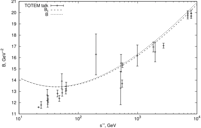
Both real and imaginary parts of the amplitude are analytically prescribed by the kfk-model. That allows one to calculate the experimental characteris-tics and get direct insight into the validity of some approximations. Figure 1 reproduces the experimental data about the diffraction cone slope B(s) [26] and Figure 2 demonstrates how they are fitted by the kfk-model from ISR to LHC energies. The fit is good in general but one sees some discrepancy at low ISR energies and at TOTEM 2.76 TeV data.
Figure 2: The fit of the B-data (Fig.1) by the kfk-model (the dotted line). The dashed lineBI indicates that the slope is well accounted by the imaginary
part of the amplitude alone.
11 12 13 14 15 16 17 18 19 20 21
101 102 103 104
B, GeV
−2
s1/2
, GeV TOTEM talk
Table 1: The energy behavior of main pp-characteristics of the kfk-model
G(s,0) 0.99756 0.99998 1.00000
ΓI[0,|t0|] 0.053928 0.054432 0.047289
kfk-model. This ”anatomy” answers the question raised at the title of the section.
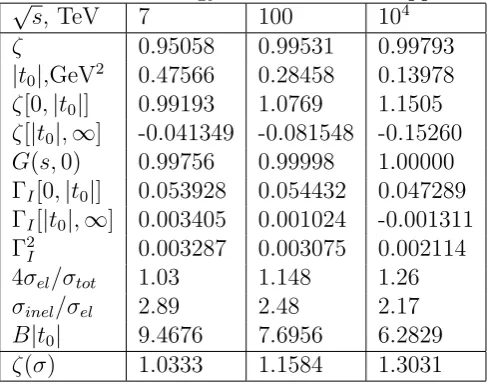
The exact value ofζ(s) is crucial for our conclusions, especially ifζ closely approaches 1 as occurs at LHC energies. The integrandfI in Eq. (12) changes
sign for the kfk-model as demonstrated at 7 TeV and 104 TeV in Figure 3.
The energy dependence of its zeros t=t0(s) has been computed and shown
in the Table. The contributions toζ from the positive and negative branches of the integrand are also shown there as ζ[0,|t0|] and ζ[|t0|,∞]. The first of
them exceeds 1 at high energies and would deplete the inelastic profile at the center if not compensated by the second one. The numerical contribution of the negative tail is very small but it is decisive for the asymptotic behavior of ζ which approaches 1 and does not exceed it. Thus the central profile saturates withG(s,0) tending to 1 (see the Table). The whole profile becomes more Black, Edgier and Larger (the BEL-regime [27]) similar to the tendency observed from ISR to LHC energies (see Fig. 7 in [3]). Nothing drastic happens in asymptopia!
The share of elastic processes and their ratio to inelastic collisions com-puted according to the kfk-model are also shown in the Table. Let us stress again that in the kfk-model the ratior = 4σel/σtotbecomes larger than 1 with
increasing energy while ζ saturates at 1 as shown in the Table. This differ-ence is crucial for asymptotic predictions about the shape of the interaction region.
Figure 3: The t-dependence of fI at 7 TeV and at 104 TeV (the kfk-model).
The positions of zeros are shown.
−5 0 5 10 15 20 25 30
0.2 0.4 0.6 0.8 1 1.2 1.4 1.6 1.8 2
|t0|
|t0|
fI
|t|, GeV2
kfk s1/2
=7TeV
kfk s1/2
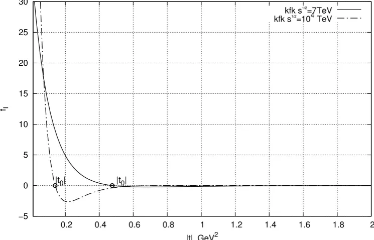
Figure 4: The value of B|t0| decreases with energy (the kfk-model).
0 0.2 0.4 0.6 0.8 1 1.2 1.4 1.6 1.8 2 2.2
101 102 103 104 105 106 107
B|t
0
|
s1/2
, GeV
kfk
model. They happen to be negligibly small as seen from the Table at ΓI
[...]-and Γ2
I-lines.
It is interesting to note, that, according to the kfk-model, the contribu-tion of the imaginary part to the differential cross seccontribu-tion dominates almost everywhere except the very narrow region near the dip (see Fig. 3 in [3]). This is also true at those transferred momenta where fI becomes negative.
We do not consider in detail the whole impact-parameter shape of the interaction region here because, for our purposes, it was enough to consider it at the most sensitive point of central collisions at b = 0. Moreover, it has been done in the references [7, 20, 21, 22, 23, 24].
6
Comparison to some other models
There is no shortage of models of elastic scattering on the market nowa-days. We want just to stress that the kfk-model provides explicit analytical expressions for the amplitude both in transferred momenta and in impact parameters.
the predictions of the BSW-model [28] in Refs [2, 3] and with Selyugin-model [29] in Ref. [3] at energies 7 and 14 TeV. In the measured interval of the transferred momenta they almost coincide within the experimental uncertainties. The results of the models are slightly different in the shapes at larger (not measured yet) transferred momenta due to the different number of predicted zeros of the amplitude.
The two most important features of the experimental data are well re-produced by the kfk-model. Those are the slope of the diffraction cone and the dip position which coincides practically with the zero of the imag-inary part of the amplitude. Therefore, to get the easier insight, one can oversimplify the model leaving only these two parameters [30] and writing fI ∝(1−(t/t0)2) exp(Bt/2) with the slope B = (BI+ρ2BR)/(1 +ρ2)≈BI.
This toy-model admits to calculate analytically the relation between r and ζ: is important that their ratio (17) depends on a single parameter Bt0 which
shows how deeply the dip penetrates inside the cone. The excess becomes larger at higher energies because (Bt0)2 decreases as seen from the Table and
Figure 4. It can be used as a guide in comparing further results at higher energies.
Measuring the differential cross section, we get no information about the signs of real and imaginary parts of the amplitude. The kfk-model predicts that the imaginary part changes its sign near the dip of the differential cross section. In principle, one can imagine another possibility to fit the differential cross section ascribing positive fI(s, t) ∝ +
p
dσ/dt, i.e. considering the positive tail of fI. Unfortunately, it lacks any explanation of the dip in the
differential cross section as a zero of the imaginary part. This assumption was used in papers [7, 20, 21, 22, 23, 24]. Since the kfk-model claims to describe the tail of the differential cross section quite well, the proposal of positivefI
would mean that one should just subtractζ[|t0|,∞] fromζ[0,|t0|]. The result
the +pdσ/dt-case. The predicted increase of ζ is somewhat slower than in the previous case but the asymptotic depletion of the inelastic profile is confirmed.
At present energies the values of ζ and r differ by about 5%. Thus, the quadratically small decline of G(s,0) from 1 claimed in [24] can not be noticed within the accuracy of experimental data. The choice between different possibilities could be done if the drastic change of the exponential shape of the diffraction cone at higher energies will be observed at higher energies. Some guide to that is provided in the kfk-model by the rapid motion of the positions of zeros inside the cone with energy increase as seen from the Table and from the simplified treatment [30]. It is interesting to note that a slight decline from the exponentially falling t-shape of the diffraction peak was shown by the extremely precise data of the TOTEM collaboration [10] already at 8 TeV. Is that the very first signature?
It was proposed [31] to explain this decline as an effect of t-channel uni-tarity with the pion loop inserted in the Pomeron exchange graph. The s-channel ”Cutkosky cut” of such a graph (its imaginary part) reproduces exactly the inelastic one-pion exchange graph first considered in [1]. Thus the external one-pion shell ascribed to inelastic peripheral interactions almost 60 years ago becomes observable at small t of the elastic amplitude at 8 TeV.
Moreover, the energy behavior of the slopeB(s) looks somewhat different from the logarithmical one prescribed to it by the Regge-poles. The transition between 2.76 TeV and 8 TeV data would ask for steeper dependence (see Figure 1) and, therefore, for a non-pole nature of the Pomeron singularity.
7
How different
b
-regions contribute to the
t
-structure of the elastic amplitude
Here we can only rely on the kfk-model where the analytical expression for the amplitude in the b-representation (4) is written. We demonstrate the evolution with energy increase of the imaginary part of the amplitude as a function of the transferred momentum in Figure 5 for the presently avail-able energy 7 TeV (upper part) and for ”asymptotically” high energy 104
TeV (lower part) by the dash-dotted lines. It is clearly seen that the diffrac-tion cone becomes much steeper and the zero moves to smaller transferred momenta at higher energies.
b-space shape of the amplitude (4). The region of small impact parameters is up to values of b ≤ 2.5 GeV−1 ≈ 0.5 fm. Here the exponential term is at
least twice higher than ΨK (see Fig. 7b in Ref. [2]). Its contribution tofI is
shown by the solid line in Figure 5. The region of large impact parameters (dotted line) is considered at distances above 1 fm. The intermediate region (dashed line) lies in between them (2.5 - 6 GeV−1).
The most intriguing pattern is formed inside the diffraction cone. The intermediate region of impact parametersb(2.5-6 GeV−1) contributes mainly
there (especially for 0.15<|t|<0.4 GeV2) at 7 TeV. However quite sizable
contributions appear from small impact parameters at 0.07 < |t| < 0.15 GeV2 and, especially, from large impact parameters at very small |t|<0.07
GeV2.
At 104 TeV the peripheral region of large impact parameters strongly
dominates at very small|t|while the role of central interactions is diminished. The remarkable feature of the kfk-model, its zero of fI, appears due
to compensations from small and medium impact parameters at 7 TeV for |t| ≈ 0.5 GeV2. The peripheral region does not play an important role in
its existence. In contrast to it, namely peripheral contribution is crucial at 104 TeV. It is compensated by the sum from the intermediate and central
regions of the impact parameters at |t| ≈0.1 GeV2.
At larger|t|the damped oscillatory pattern of contributions from interme-diate and peripheral regions of b dominates at all energies while the steadily decreasing (with |t|) share of central interactions is rather unimportant.
Figure 5: The shapes of the imaginary part as a function of the transferred momentum at 7 TeV (up) and 104TeV (below) are shown by the dash-dotted
lines. The contributions to them from different impact parameters are also shown.
Elastic scattering of protons continues to surprise us through new experi-mental findings. The implications of the peculiar shape of the differential cross section and the increase of the ratio of the elastic to total cross sec-tions with increasing energy are discussed above. These facts determine the spatial interaction region of protons. Its shape can be found from the unitar-ity condition within definite assumptions about the behavior of the elastic scattering amplitude. The inelastic interaction region becomes more Black, Edgier and Larger (BEL) in the energy range from ISR to LHC. Its further fate at higher energies is especially interesting.
the difference between these two possibilities. It is negative in the kfk-model and positive for a different prescription. That can not be found from exper-iment and asks for phenomenological models. The energy behavior of the ratio of elastic to total cross sections plays a crucial role. If observed, its rapid increase at higher energies would give some arguments in favor of the second possibility.
More surprises could be in store for us from the evolution of the shape of the diffraction cone with the dip position moving inside it and a drastic change of its slope as shown above. First signatures of the shape evolution can be guessed even at present energies from TOTEM-findings at 2.76 TeV and 8 TeV.
Acknowledgments
I.D. is grateful for support by the RAS-CERN program and the Compet-itiveness Program of NRNU ”MEPhI” ( M.H.U.).
References
[1] I.M. Dremin, D.S. Chernavsky, JETP 38 (1960) 229
[2] A.K. Kohara, E. Ferreira, T. Kodama, Eur. Phys. J. C 73 (2013) 2326
[3] A.K. Kohara, E. Ferreira, T. Kodama, Eur. Phys. J. C 74 (2014) 3175
[4] H.G. Dosch, Phys. Lett. B 199(1987) 177
[5] H.G. Dosch, E. Ferreira, A. Kramer, Phys. Rev. D 50 (1994) 1992
[6] E. Ferreira, F. Pereira, Phys. Rev. D 61 (2000) 077507
[7] U. Amaldi, K.R. Schubert, Nucl. Phys. B 166 (1980) 301
[8] G. Antchev et al.[TOTEM Collaboration], Europhys. Lett. 96 (2011) 21002
[9] G. Antchev et al. [TOTEM Collaboration], Europhys. Lett.101 (2013) 21002
[10] G. Antchev et al. [TOTEM Collaboration], Nucl. Phys. B 899 (2015) 527
[12] T. Cs¨org¨o, [TOTEM Collaboration], arXiv:1602.00219
[13] G. Aad et al. [ATLAS Collaboration], Nucl. Phys. B 889 (2014) 486
[14] M. Aaboud et al. [ATLAS Collaboration], Phys. Lett. B761 (2016) 158
[15] PDG group, China Phys. C 38 (2014) 090513
[16] I.M. Dremin, Physics-Uspekhi 56 (2013) 3; ibid. 58 (2015) 61; ibid. 60
(2017) 362
[17] L. Van Hove, Nuovo Cimento 28 (1963) 798
[18] A. Martin, Lett. Nuovo Cimento 7 (1973) 811
[19] A. Martin, Phys. Lett. B 404 (1997) 137
[20] I.M. Dremin, V.A. Nechitailo, Nucl. Phys. A 916 (2013) 241
[21] I.M. Dremin, Int. J. Mod. Phys. A 31 (2016) 1650107
[22] I.M. Dremin, S.N. White, The interaction region of high energy protons; arXiv 1604.03469.
[23] S.N. White, Talk at the conference QCD at
Cosmic Energies, Chalkida, Greece, May 2016;
http://www.lpthe.jussieu.fr/cosmic2016/TALKS/White.pdf
[24] A. Alkin, E. Martynov, O. Kovalenko, S.M. Troshin, Phys. Rev. D 89
(2014) 091501(R)
[25] I.V. Andreev, I.M. Dremin, ZhETF Pis’ma 6 (1967) 810
[26] S. Giani, TOTEM Experiment Report, CERN-PRB-2017-043, 25 April 2017
[27] R. Henzi, P. Valin, Phys. Lett B 132 (1983) 443
[28] C. Bourrely, J.M. Myers, J. Soffer, T.T. Wu, Phys. Rev. D 85 (2012) 096009
[29] O.V. Selyugin, Eur. Phys. J. C 72 (2012) 2073
[30] I.M. Dremin, Int. J. Mod. Phys. A 32 (2017) 1750073
[31] L. Jenkovszky, I. Szanyi, Mod. Phys. Lett. A 32 (2017) 1750116
![Figure 1: The experimental data about the diffraction cone slope B(s) [26].](https://thumb-ap.123doks.com/thumbv2/123dok/2962601.1356465/8.595.110.484.233.623/figure-experimental-data-diraction-cone-slope-b-s.webp)