Advanced Dynamic system Simulation Free ebook download

(1)

(2)

Advanced Dynamic-system

Simulation

Model-replication Techniques and

Monte Carlo Simulation

Granino A. Korn

University of Arizona Tucson, Arizona

WILEY-INTERSCIENCE

(3)

(4)

(5)

(6)

Advanced Dynamic-system

Simulation

Model-replication Techniques and

Monte Carlo Simulation

Granino A. Korn

University of Arizona Tucson, Arizona

WILEY-INTERSCIENCE

(7)

Published by John Wiley & Sons, Inc., Hoboken, New Jersey Published simultaneously in Canada

No part of this publication may be reproduced, stored in a retrieval system, or transmitted in any form or by any means, electronic, mechanical, photocopying, recording, scanning, or otherwise, except as permitted under Section 107 or 108 of the 1976 United States Copyright Act, without either the prior written permission of the Publisher, or authorization through payment of the appropriate per-copy fee to the Copyright Clearance Center, Inc., 222 Rosewood Drive, Danvers, MA 01923, 978-750-8400, fax 978-750-4470, or on the web at www.copyright.com. Requests to the Publisher for permission should be addressed to the Permissions Department, John Wiley & Sons, Inc., 111 River Street, Hoboken, NJ 07030, 201-748-6011, fax 201-748-6008, or online at http://www.wiley.com/go/permission.

Limit of Liability/Disclaimer of Warranty: While the publisher and author have used their best efforts in preparing this book, they make no representations or warranties with respect to the accuracy or completeness of the contents of this book and specifically disclaim any implied warranties of merchantability or fitness for a particular purpose. No warranty may be created or extended by sales representatives or written sales materials. The advice and strategies contained herein may not be suitable for your situation. You should consult with a professional where appropriate. Neither the publisher nor author shall be liable for any loss of profit or any other commercial damages, including but not limited to special, incidental, consequential, or other damages.

For general information on our other products and services or for technical support, please contact our Customer Care Department within the United States at 877-762-2974, outside the United States at 317-572-3993 or fax 317-572-4002.

Wiley also publishes its books in a variety of electronic formats. Some content that appears in print may not be available in electronic formats. For more information about Wiley products, visit our web site at www.wiley.com.

Library of Congress Cataloging-in-Publication Data:

Korn, Granino Arthur,

1922-Advanced dynamic-system simulation : model-replication techniques and Monte Carlo simulation / by Granino A. Korn.

p. cm. Includes index.

ISBN 978-0-470-08188-4 (cloth/cd)

1. System analysis--Simulation methods. 2. Monte Carlo method. I. Title. QA402. K665 2007

003' .85-- dc22

200601618

(8)

v

Preface

Simulation is experimentation with models. This book describes new com-puter programs for interactive modeling and simulation of dynamic systems, such as aerospace vehicles, control systems, and biological systems. Simulation studies for design or research can involve many hundreds of model changes, so programming must be convenient, and computations must be as fast as possible.

This book is about advanced simulation programming and describes many new techniques. We provide only a brief review of routine simulation pro-gramming but demonstrate computer software for remarkably fast and respectably large simulation studies on inexpensive personal computers or workstations. For hands-on experiments, the enclosed CD contains an indus-trial-strength software package rather than a toy demonstration program.1

1_{OPEN DESIRE solves up to 40,000 ordinary differential equations under Linux, and up to}

20,0000 differential equations under Microsoft WindowsTM, so that one can implement respectable vectorized Monte Carlo studies. The DESIRE language, widely used since 1985, accepts scalar and vector differential equations and difference equations in a natural mathe-matical notation, for example,

d/dt x = – x * cos(w * t) + 2.22 * a * x Vector y = A * x + B * u

(17)

xiv Preface

The included OPEN DESIRE program for Linux solves up to 40,000 ordi-nary differential equations and implements exceptionally fast and convenient vector operations. A smaller educational 20,000 differential-equations ver-sion for Microsoft WindowsTM can be obtained without charge from the author by sending an email to gatmkorn@aol.com. The user can run, edit, and modify the example simulations keyed to the figures in this book, plus many other examples. Many of our programming principles also apply to simulation programs other than DESIRE.

Chapter 1 introduces our subject with a few programs for small differen-tial-equation models, including a simple guided-missile simulation. The remainder of the book presents new material. Chapter 2 begins with a careful discussion of models that involve sampled-data operations and sampled-data difference equations together with differential equations. We model mixed analog–digital systems such as simulated digital controllers and systems with limiters and switches. At this point, we show that many very useful devices (e.g., track-hold circuits, trigger circuits, signal generators, automatic scal-ing) are neatly and efficiently modeled with simple difference equations. Last, but not least, we propose improved techniques for proper numerical integration of switched variables.

Truly powerful simulation programs need a readable notation for vector and matrix assignments, differential equations, and difference equations. Chapter 3 introduces a novel vector compiler that produces very fast pro-grams for vector and matrix operations. We also demonstrate efficient use of submodels. We present examples from control engineering and nuclear-reac-tor simulation. The following chapter then shows how we use vecnuclear-reac-tors to repli-cate complete models.

Chapter 4 describes practical model replication (vectorization): a single sim-ulation run with a vector model will replace hundreds or thousands of conven-tional simulation runs. We apply the vectorizing compiler introduced in Chapter 3 to parameter-influence studies and Monte Carlo simulation of dynamic sys-tems with noise-perturbed parameters and random initial conditions. We com-pare repeated-run and vectorized Monte Carlo studies of a weapon trajectory. Our interactive programs produce not just time histories of system variables but also time histories of statistics such as averages, mean squares, and probability estimates. We also show explicitly how to estimate probability densities.

(18)

Chapter 6 discusses vector models of neural networks including a new pulsed-neuron model. Chapter 7 deals with vectorized programs for fuzzy-set controllers, partial differential equations, and agroecological models repli-cated at many points of a landscape map. The Appendix gets a small selection of reference material out of the way of the main text.

GRANINOA. KORN

Chelan, Washington

October 2006

(19)

(20)

1

Introduction to

Dynamic-system Simulation

DYNAMIC-SYSTEM MODELS AND COMPUTER PROGRAMS

1-1. Computer Modeling and Simulation

Simulation is experimentation with models. Simulation for engineering design, research, and education studies must rapidly exercise a wide variety of models and then store and access a large volume of results. This is practi-cal only with models programmed on computers.

Dynamic-system modelsrelate model-system states to earlier states. Classical physics, for example, predicts continuous changes of quantities such as position, velocity, or voltage with continuous time. Computer simulation of such systems started in the aerospace industry and is now indispensable in biology, medicine, and agroecology as well as in all engineering disciplines. At the same time, dis-crete-event simulation has gained importance for business and military planning. Simulation is at its best when combined with mathematical analyses. But simulation results can often provide insight and possibly useful decisions where exact analysis is impractical. This was true for many early control-system optimizations. As another example, Monte Carlo simulations simple-mindedly measure statistics over repeated experiments to solve problems that are too complicated for probability theory analysis. Simulation results must eventually be validated by real experiments, just like analytical results.

1 Advanced Dynamic-system Simulation: Model-replication Techniques

(21)

2 Introduction to Dynamic-system Simulation

Computer simulations can be speeded up or slowed down at the experi-menter’s convenience. You can simulate a flight to Mars or to Alpha Centauri in one second. Periodic clock interrupts synchronizing suitably scaled simu-lations with real time permit “hardware in the loop”: you can “fly” a real autopilot—or a real human pilot—on a tilting platform controlled by a com-puter flight simulation. In this book, we are interested in very fast simulation, for we want to study the effects of many different model changes. Specifically, we want to

1. Enter and edit programs in convenient editor windows.

2. Use typed or graphical-interface commands to start, stop, and pause simulations, to select displays, and to make parameter changes. Results ought to appear immediately to provide an intuitive “feel” for the effects of model changes (interactive modeling).

3. Program systematic parameter-influence studies and produce cross-plots or tables.

4. Program model changes to optimize effectiveness measures, and study effects of random parameter changes or random model inputs by taking statistics on repeated simulations (Monte Carlo simulation).

1-2. Differential-equation Models

Continuous-system simulation models delayed interactions of physical state variables x1, x2, … with first-order ordinary differential equations (state equations)

(d/dt) xi = fi(t; x1, x2, …; y1, y2, …; a1, a2, …) (i = 1, 2, …) (1-1a)

Heretrepresents the time, and the quantities

yj = gj(t; x1, x2, ...; y1, y2, …; b1, b2, …) (j = 1, 2, …) (1-1b)

are defined variables. a1, a2, …, and b1, b2, … are constant model parameters.

(22)

The state variables xiare system outputs. They start at t = t0with given initial values; subsequent values are produced by an integration routine (Section 1-7) from the fi-values generated by the preceding execution (derivative call) of the operations (1).

There are three kinds of defined variables yj:

1. system inputs (specified functions of the timet) 2. system outputs

3. intermediate results needed to compute the derivatives fi

It must be possible to sort the defined-variable assignments (1-1b) into a pro-cedure that successively derives all the yjfrom state variables xiand/or the timetwithout recurrence relations or “algebraic loops” (Section 1-9).

Some dynamic systems (e.g., systems involving interconnected mechani-cal devices in automotive engineering and robotics) are modeled with differ-ential-equation systems that cannot be explicitly solved for state-variable derivatives as in Eq. (1-1). Simulation then requires solution of algebraic equations at each integration step. Such differential-algebraic-equation (DAE) systems are not treated in this book. References [1–4] describe suit-able mathematical methods and special software.

1-3. Interactive Modeling—Experiment Protocol and Simulation Studies

Practical computer simulation is not simply a matter of programming and solving model equations. We must also make it convenient to modify our models and try many different experiments (see also Section 1-5). In addition to DYNAMIC program segments listing the model equations (1-1), each sim-ulation study requires an experiment protocol program that sets and changes initial conditions and model parameters, calls computer runs, and displays or tabulates solutions for different model configurations.

The simplest experiment protocols are just sequences of successive commands, say

a = 20.0 | b = – 3.35 (set parameter values)

x = 12.0 (set the initial value of x)

drun (make a differential-equation -solving simulation run)

reset (reset initial values)

a = 20.1 (change model parameters)

b = b – 2.2

drun (try another run)

(23)

Eachdruncommand calls a differential-equation-solving simulation run, and resetresets initial conditions. Typed commands ought to execute immediately to permit interactive modeling. The operator inspects the solution output after each simulation run and then types new commands for the next run. Command-mode operation also permits interactive program debugging [5].

A simulation study combines such commands into a storable program seg-ment (experiseg-ment-protocol script) that can branch and loop to call repeated simulation runs for different parameter combinations. Simulation studies may involve thousands of model and parameter changes, so programming must be easy and computations must be as fast as possible. This is why we like to interpret experiment-protocol scripts and compile the program seg-ments executing the actual simulation runs.

1-4. Simulation Software

Commercially available equation-oriented simulation programs such as ACSLTM _{accept system equations in a more or less human-readable form,}

sort defined variable assignments as needed, and feed the sorted equations to an optimizing Fortran or c compiler [5]. Berkeley Madonna and DESIRE (see below) have built-in equation-language compilers and execute immedi-ately. Block-diagram interpreters (e.g., SimulinkTM_{, Vissim}TM_{, and the}

open-source program Scicos) permit graphical block-diagram composition and immediately execute interpreted simulation runs. Such programs usually pro-vide equation-language blocks for complicated expressions. Interpreted code is slow; production runs are sometimes translated into c for faster execution. Alternatively, ACSLTM_{, Easy5}TM_{, and Berkeley Madonna have block-diagram}

preprocessors for compiled simulation programs. More advanced modeling is possible with the Modelica language [6–8].

1-5. OPEN DESIRE and DESIRE

The simulation programs described in this book, and, in particular, our new techniques for model replication (vectorization), Monte Carlo simulation, and submodels (Chapters 3–7), use the open-software simulation package OPEN DESIRE for Linux, Unix including Cygwin (Unix under Windows), and Microsoft WindowsTM_{, or the commercially available DESIRE/2000}

program for Windows.1DESIRE simulation systems allow inexpensive per-sonal computers and workstations solve thousands of differential equations in seconds.

1_{The earlier (1995) Windows version of DESIRE discussed in References [1,2] lacks the}

(24)

How a Simulation Run Works 5 DESIRE uses double-precision (64-bit) floating-point arithmetic and accepts command scripts and model descriptions in a readable mathematical notation such as

y = a cos(x) + b d/dt x = – x + 4 y

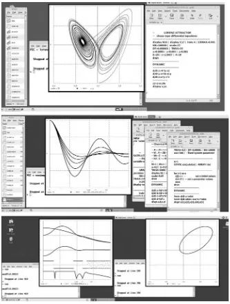
Command scripts can include operating-system calls, shell scripts, and calls to other computer programs. DESIRE’s command-script language is itself a general-purpose mathematical language and handles vectors, matrices, and even complex numbers (e.g., for frequency-response and root-locus plots) [9]. Programs are entered and edited in editor windows (Fig. 1-1). Each program begins with an experiment-protocol script that is interpreted much like an advanced Basic dialect. When the experiment-protocol script encounters a drun statement, a built-in runtime compiler automatically compiles a DYNAMIC program segment listing model equations. The state-equation-solving simulation run then executes at once and produces solution displays in bright color.

Very fast compilation (typically under 50 ms) simplifies interactive mod-eling. Experimenters can immediately observe results of programmed or screen-edited models and experiment-protocol changes. One can enter and edit different models in multiple editor windows and run these models in turn to compare results (Fig. 1-1). Runtime displays show solution time histories and error messages during rather than after each simulation run, so that you can save time by aborting undesirable runs before they complete.

The experiment-protocol script starting each DESIRE program defines an experiment. Subsequent DYNAMIC program segments define models used in the experiment and specify runtime input/output requests. An experiment protocol can call multiple DYNAMIC segments with different models, dif-ferent versions of the same model, and/or difdif-ferent input/output operations.

HOW A SIMULATION RUN WORKS

1-6. Sampling the DYNAMIC Segment Variables

Whendruncalls a simulation run, the program initializes input/output opera-tions requested by the DYNAMIC program segment. The independent variable t(simulation time) and the differential-equation state variables start with initial values assigned by the experiment protocol.2 _{A first pass through the}

DYNAMIC-segment code [Eq. (1-1)] produces initial values of the defined

2_{Unspecified initial values of unsubscripted differential-equation state variables conveniently}

(25)

(26)

How a Simulation Run Works 7

FIGURE 1-1b. DESIRE on a dual WindowsTMscreen showing a file manager window, two editor windows, and a command Window. The red OK button on each DESIRE editor window transfers the selected edited program to DESIRE. This makes it convenient to compare two or more programs.

FIGURE 1-1c. Cygwin (Unix under WindowsTM_{) display with a Unix console window, the}

(27)

variables [Eq. (1-1b)]. Unless stopped, simulations run from the initial time t = t0tot = t0 + TMAX. You can stop a simulation run by typing ctrl candspace (zzunder Windows), and restart or extend a run with drun.

DESIRE normally samples DYNAMIC-segment variables for output (usu-ally to displays) or sampled-data operations at NN uniformly spaced sam-pling times (communication times):

t = t0, t0 + COMINT, t0 + 2 COMINT, … ,

t0 + (NN – 1)COMINT = t0 + TMAX (1-2a)

with

COMINT = TMAX/(NN – 1) (1-2b)

The experiment-protocol script sets appropriate values of t0,TMAX, and NNor uses default values listed in the DESIRE manual.

If the DYNAMIC program segment contains differential equations (d/dt orVectr d/dtstatements), then t0 defaults to t0 = 0unless another value is specified. Starting at t = t0, the integration routine increments tby successive constant or variable DTsteps untiltreaches the next data-sampling commu-nication point (Fig. 1-2a). Within each integration step, numerical integration 8 Introduction to Dynamic-system Simulation

x

x (t)

DT COMINT

t0 t0+COMINT t0+2 COMINT t0+TMAX

t

(28)

approximates continuous updating of the “continuous” model variables t, xi, andyj. Each integration step usually requires more than one derivative call executing the model equations (1-1) (Section 1-7; [10–18]).

In DYNAMIC program segments without differential equations, t0 defaults to t0 = 1unless the experiment-protocol script specifies a different value. All operations in such a DYNAMIC segment are sampled-data assign-ments and execute at successive communication times [Eq. (1-2)], except for assignments preceded by aSAMPLE mstatement, where mis an integer >1. Such assignments execute only at t = t0and then at every mth_{communication}

point. This permits multirate sampling. DESIRE admits only one SAMPLE mstatement per DYNAMIC program segment.

Differential-equation-solving DYNAMIC segments can also include sam-pled-data assignments that execute only at the periodic sampling points (1-2). Such assignments model sampled-data controllers and noise generators and must be collected in sections following an OUTand/orSAMPLE mstatement at the end of the DYNAMIC program segment (Section 2-3).

DYNAMIC-segment input/output (e.g., to displays and listings) occurs at the NNcommunication points (1-2), unless the system variable MM, which defaults to 1, is set to an integer >1. In this case, input/output occurs at t = t0, then at every MMth_{sampling point, and finally at t = t0 + TMAX. NN}_{can thus}

be set to a larger value than the desired number of input/output points. This

How a Simulation Run Works 9

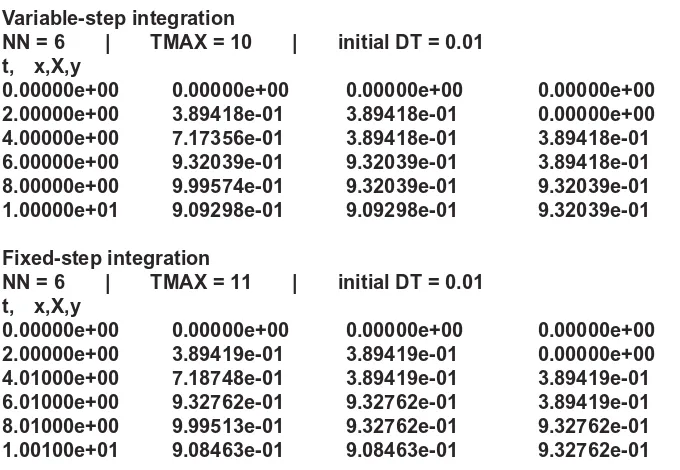
FIGURE 1-2b. DESIRE output listings for variable-step integration and for fixed-step integration. Parameters were deliberately chosen to exaggerate the fixed-DTeffect.

Variable-step integration

NN = 6 | TMAX = 10 | initial DT = 0.01 t, x,X,y

0.00000e+00 0.00000e+00 0.00000e+00 0.00000e+00 2.00000e+00 3.89418e-01 3.89418e-01 0.00000e+00 4.00000e+00 7.17356e-01 3.89418e-01 3.89418e-01 6.00000e+00 9.32039e-01 9.32039e-01 3.89418e-01 8.00000e+00 9.99574e-01 9.32039e-01 9.32039e-01 1.00000e+01 9.09298e-01 9.09298e-01 9.32039e-01

Fixed-step integration

NN = 6 | TMAX = 11 | initial DT = 0.01 t, x,X,y

(29)

can provide fast sampling for pseudorandom noise (Section 5-4) and/or for sampling switch and limiter functions (Sections 2-10 and 2-11).

Some defined-variable assignments (1-1b) do not affect state variables but only scale or modify model output. Such operations are not needed at every derivative call but only at sampling points. The simulation will run faster if such assignments are programmed as sampled-data operations following an OUTstatement.

1-7. Numerical Integration

(a) Euler Integration

The simplest procedure that approximates continuous updating of a state variable xin successive integration steps is the explicit Euler integration rule (see also Appendix)

xi(t + DT) = xi(t) + fi[t; x1(t), x2(t), ...; y1(t), y2(t),... ]DT

(i = 1, 2, …, n) (1-3)

wherefiis the value of dx/dtcalculated by the derivative call executing Eq. (1-1) at the time t.

The integration routine loops until treaches the next communication point (1-2), where the solution is sampled for input/output and sampled-data oper-ations. The simulation run terminates after accessing the last sample at t = t0 + TMAX unless the run is stopped either by the user or by a programmed termination (term) statement.

(b) Improved Integration Rules

The Euler integration rule [Eq. (1-3)] simply increments each state variable by an amount proportional to its last computed derivative. This does not approximate true integration well except for very small integration steps DT. Improved updating requires multiple derivative calls per integration step DT [10–18]. This can actually reduce the total number of derivative calls (the main computing load of a simulation) required for a specified accuracy. In particular:

• Multistep rulesextrapolate updated values of the xias polynomials based on values of the xiandfiat several past times t – DT, t – 2DT, ….

• Runge–Kutta rules precompute two or more approximate derivative values in the interval (t, t + DT)by Euler-type steps and use their weighted aver-age for updating.

(30)

Coefficients in such integration formulas are chosen so that polynomials of degree Nintegrate exactly (Nth_{-order integration formula).}

Explicit integration rules such as Eq. (1-3) express future values xi(t + DT) in terms of already computed past state-variable values. Implicit rules, such as the implicit Euler rule,

xi(t + DT) = xi(t) + fi[t + DT; x1(t + DT), x2(t + DT), ...;

y1(t + DT), y2(t + DT), ...] DT (i = 1, 2, ..., n) (1-4)

require a program that solves the predictor equation (1-4) for xi(t + DT) at each step. Implicit rules clearly involve more computation, but they may admit larger DTvalues without numerical instability.

Variable-step integration adjusts integration step sizes to maintain accu-racy estimates obtained by comparing various tentative updated solution val-ues. This can save many steps. Figures 1-5, 7-7, and 7-8 show examples. Numerical integration normally assumes integrands fithat are continuous and differentiable within each integration step. Step-function inputs are accept-able only at t = t0and thereafter at the end of integration steps. Sections 2-10 to 2-12 discuss this problem in connection with models involving sampled-data operations and switching functions.

1-8. Sampling Times and Integration Steps

The experiment protocol script selects the simulation runtime TMAXand the number of samples NN needed for display, listings, and/or sampled-data models. DESIRE returns an error message if an integration-step value DT larger than COMINT = TMAX/(NN – 1)is selected, for the program must never sample data within integration steps. Sampled-data output to displays or sam-pled-data assignments is not well-defined at such times. Samsam-pled-data input within integration steps might make the numerical-integration routine invalid (see also Sections 2-9 to 2-11).

DESIRE’s variable-step integration routines automatically force the last integration step in each communication interval to end precisely on one of the user-selected communication points (1-2). An error message warns if the initial DT value exceeds COMINT. Fixed-step integration routines, however, may have to add a fraction of DTto each sampling time (1-2) to make sure that sam-pling always occurs at the end of an integration step, as shown in Eq. (1-2b). This does not cause errors in displays or listings, for each x(t)value is still asso-ciated with its correct tvalue. But if output listings at specified periodic sam-pling times (1-2) are needed, one must either use variable-step integration or set DTto a very small integral fraction of COMINT.

(31)

1-9. Sorting Defined-variable Assignments

DYNAMIC-segment operations (1-1) preceding an OUTorSAMPLE m state-ment (if any) execute at every derivative call of the differential-equation-solv-ing integration routine. Each derivative or defined-variable assignment uses the value of tand the values of the state variables xicomputed by the last deriva-tive call. Derivaderiva-tive and defined-variable values for t = t0are derived from the initial state-variable values and t0by an extra initial derivative call.

The defined-variable assignments (1-1b) must execute in the correct pro-cedural order to derive each yjvalue from the state-variable values and t, pos-sibly using already computed yivalues. An out-of-order assignment would incorrectly try to use defined-variable values from an earlier derivative call. The state equations (1-1a) are normally programmed following the defined-variable assignments (1-1b).

Conventional simulation programs such as ACSL©automatically sort the defined-variable assignments so that they use only yivalues already com-puted during the current derivative call. If that is impossible due to an “alge-braic loop,” the program returns an error message (sort error). DESIRE’s more general program system does not sort statements automatically. But in programs without subscripted variables or vectors (Chapter 3), DESIRE pre-vents assignments to undefined variables, and thus algebraic loops, by return-ing an error message (see also Section 3-5).3

EXAMPLES OF SIMPLE APPLICATIONS

1-10. Oscillators and Computer Displays

(a) A Linear Harmonic Oscillator

The complete small program in Figure 1-3 illustrates the main features of a DESIRE simulation. The DYNAMIC program segment following the DYNAMICstatement in Figure 1-3adefines our model. We have modeled a simple damped harmonic oscillator or mass–spring–dashpot system with the differential equations

d/dt x = xdot | d/dt xdot = – ww * x – r * xdot 12 Introduction to Dynamic-system Simulation

3_{Recursive assignments that input the assigned-to variable on the right-hand side, as in}

y = y + x y = a * x1 + y * x2

(32)

Examples of Simple Applications 13

+

0

-0 5 → 10

scale = 1 x vs. t

FIGURE 1-3a. This complete simulation program for a linear oscillator produces five simu-lation runs with different values of the damping coefficient r.

A LINEAR OSCILLATOR ---display N1 | display C8 | display Q TMAX = 10 | DT = 0.0001 | NN = 10001

ww=0.8 | -- parameter value

x = 1 | -- initial value

---for i = 1 to 5 | -- set parameter values

r = 0.2 * i

drunr | display 2 | -- don't erase display next

---DYNAMIC

(33)

14 Introduction to Dynamic-system Simulation

+

0

– –1.0

scale = 1 –0.5 x,xdot0.0 0.5 1.0

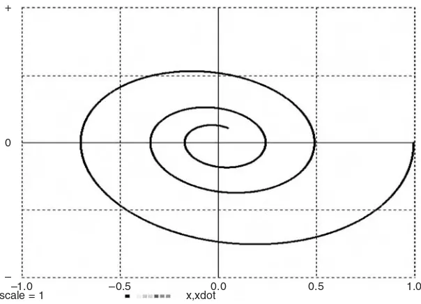
FIGURE 1-3b. A phase-plane plot (xdotversus x) for the linear oscillator in Figure 1-3a.

We can add a display specification:

• dispt x, xdot displays the variables x and xdotversus the simulation timet.

• dispxy x,xdotdisplaysxdotversus x(phase-plane plot).

Model and display are exercised by the experiment-protocol script preced-ing the DYNAMICstatement. Successive experiment-protocol lines specify

• display colors and curve thickness

• the runtimeTMAX,the integration step DT, and the number NNof dis-play points

• a model parameter ww

• the initial value of the state variable x

Initial values of time tand of the state variable xdotare not specified and default to 0. The integration routine defaults to a fixed-step second-order Runge–Kutta rule.4

A simple experiment-protocol loop next calls for five simulation runs with five different values of the oscillator damping parameter r. The resulting displays are reproduced at the top of Figure 1-3a. Figure 1-3bshows a phase-plane plot.

4_{The OPEN DESIRE reference manual in the book CD describes the complete program}

(34)

Examples of Simple Applications 15 (b) A Nonlinear Oscillator and Duffing’s Differential Equation

The differential equations

d/dt x = xdot | d/dt xdot = – x * x * x – a * xdot

model an oscillator with a nonlinear spring. Figures 1-4a and b show the resulting time histories and a phase-plane plot obtained with a = 0.02. These results are clearly different from the linear-oscillator response in Figure 1-3. If we drive the nonlinear oscillator with a sinusoidal voltage b cos(t), we obtain Duffing’s differential-equation system

d/dt x = xdot | d/dt xdot = – x * x * x – a * xdot + b * cos(t)

Figure 1-4bshows solution displays and a program. The experiment-protocol script is interesting in that it first calls a simulation run to exhibit the initial tran-sient, then a long simulation run with the display turned off to establish steady-state conditions, and finally a third run to display the steady-steady-state solution.

Reference [9] discusses DESIRE programs for several other small physics problems.

1-11. Space Vehicle Orbits—Variable-step Integration

The space-vehicle orbit simulation in Figure 1-5 assumes a fixed earth exert-ing a simple inverse-square-law gravitational force on the satellite; effects of planets, moons, and so on are neglected. With the sun at the coordinate ori-gin, the inverse-square-law accelerations in the xandydirections are

(d/dt) xdot = – (a/R2) x/R (d/dt) | ydot = – (a/R2) y/R

+

0

–

+

0

–

0 40 80

x

xdot

→

scale = 1 x,xdot vs. t scale = 1–1.0 –0.5 x,xdot0.0 0.5 1.0

FIGURE 1-4a. Time histories and phase-plane plot for the nonlinear oscillator modeled with

(35)

16 Introduction to Dynamic-system Simulation

→ →

+

0

–

+

0

–

–1.0 –0.5 0.0 0.5 1.0

scale = 10 X,xdot –1.0scale = 10 –0.5 X,xdot0.0 0.5 1.0 +

0

–

+

0

–

0 15 30 230 245 260

scale = 10 z,x,xdot vs. t scale = 10 z,x,xdot vs. t

-- DUFFING'S DIFFERENTIAL EQUATION

---scale = 10 | display N1 | display C8 | display Q a = 0.099 | b = 15

TMAX = 30 | DT = 0.0002 | NN = 10000 X = 0.02

drun

write "type go to continue" | STOP

TMAX = 200 | display 0 | drun

write " note how solution becomes periodic!" TMAX = 30 | display 1 | drun ---DYNAMIC

---d/dt x = xdot | d/dt xdot = - a * xdot - x * x * x + b * cos(t)

--z = cos(t)

Z = 0.5 * (z + scale) | X = 0.5 * x | XDOT = 0.5 * (xdot - scale) dispt Z, X, XDOT

(36)

Examples of Simple Applications 17

+

0

–

+

y

25 DT

0

–

–1.0 –0.5 0.0 0.5 1.0

scale = 1

0 2 → 4

scale = 2 y,dt vs. t

x,y

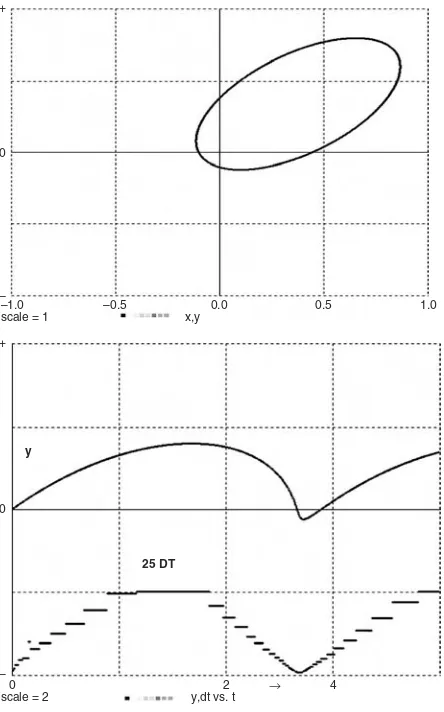
FIGURE 1-5. Space-vehicle-orbit simulation program, orbit display, and stripchart time his-tories of yandDT, showing the variable integration steps. For simplicity, the problem was scaled so that all coefficients equal unity.

-- SPACE-VEHICLE-ORBIT SIMULATION

---irule 15 | ERMAX = 0.0000001 | -- Gear-type integration

xdot = 1.4 | dot = 0.9 | x = 0.45 | y = 0 TMAX = 4 | DT = 0.0001 | NN = 10000 drun

---DYNAMIC

---rr = (x^2 + y^2)^(-1.5)

d/dt x = xdot | d/dt y = ydot

(37)

With the program scaled so that the gravitational constant a= 1, we obtain the simple differential-equation system5

rr = (x^2 + y^2)^(–1.5)

d/dt x = xdot | d/dt y = ydot

d/dt xdot = – x * rr | d/dt ydot = – y * rr

In Figure 1-5, an orbit starts around the sun to gain velocity for a trip to the outer planets. This involves dramatic velocity changes, and the small integra-tion steps required during the high-velocity porintegra-tion of the trajectory would slow the rest of the simulation. For this reason, such simulations employ an implicit variable-step/variable-order integration rule (irule 15). The second display in Figure 1-5 illustrates the integration-step changes.

1-12. A Population-dynamics Model

Typical population-dynamics models represent population counts by continu-ous differential-equation state variables. There can be any number of popula-tions, including subpopulations such as age and gender cohorts. Assignments to the state derivatives describe interactions of different populations that may breed, die, contract diseases, and fight or eat one another. Quite similar state-equation systems also describe the reaction rates of “populations” of chemical compounds or radioactive isotope mixtures (Section 7-1).

The classical example of a two-population predator–prey interaction is modeled by the Volterra–Lotka differential equations

d/dt prey = (a1 – a4 * predator) * prey d/dt predator = (– a2 + a3 * prey) * predator

The rate of increase of each population is proportional to the population size.a1is the difference between the natural birth and death rates of the prey (say of a local population of rabbits). The prey has an additional death rate a4 * predatorproportional to the size of the predator population (say a popu-lation of foxes). The predator popupopu-lation has a death rate a2, and its birth rate a3 * preyis proportional to the prey population, which is its food supply.

5 _{This Cartesian-coordinate formulation is simpler than the polar-coordinate}

differential-equation system:

x = r * cos(theta) | y = r * sin(theta)

d/dt r = rdot | d/dt rdot = - GK/(r^2) + r * thdot^2 d/dt theta = thdot | d/dt thdot = 2 * rdot * thdot/r

(38)

The simulation program in Figure 1-6 demonstrates how easily such simple population-dynamics models can be modified. We added an extra predator death rate b * predatorto account for the effect of crowding as the predator population increases and some predators kill one another. For b = 0 (no crowding) we obtain the classical periodic Volterra–Lotka solution: as the rabbits breed, the foxes have more food; their number increases until they seriously reduce the rabbit population and thus their food supply. The

+

0

–

+

0

– 0

b = 0 (no crowding)

b> 0 (crowding)

1e+03 2e+03 scale = 4000 prey,predator vs. t

→ 0 1e+03 2e+03

scale = 4000 prey,predator vs. t

→

FIGURE 1-6.A population-dynamics simulation. For b = 0the program implements the clas-sical Volterra–Lotka differential equations, which produce steady-state periodic fluctuations of the predator and prey populations. Positive values ofbmodel an increased predator death rate due to crowding, for example, by predator cannibalism. Predator and prey populations then converge to constant steady-state values.

-- A PREDATOR-PREY PROBLEM -- showing the effect of crowding

---display N1 | display C8

TMAX = 2000 | DT = 0.01 | NN = 5000 | scale = 4000 a1 = 0.05 | a2 = 0.01 | a3 = 2.0E-05 | a4 = 1.0E-04 b = 0

prey = 2000 | predator = 200 | -- initial values drunr

write " type go to see effect of predator crowding" STOP

b = 1.0E-05 | drun

---DYNAMIC

---d/dt prey = (a1 - a4 * predator) * prey

(39)

number of rabbits then increases again, and the process repeats. But crowd-ing (b > 0) limits the predator population, and both populations converge to steady-state values.

1-13. Splicing Multiple Simulation Runs: Billiard-ball Simulation

The DYNAMIC program segment in Figure 1-7 models a billiard ball as a point (x, y)on a table bounded by elastic barriers at x = a, x = – a, y = b,andy = – b. For x,ywithin the barriers, the only acceleration is due to constant friction in the negative velocity direction, so that we program

d/dt x = xdot | d/dt y = ydot

d/dt xdot = – fric * xdot/v | d/dt ydot = – fric * ydot/v

where the velocity vis obtained with the defined-variable assignment

v = sqrt(xdot^2 + ydot^2)

A differential-equation model of barrier impacts would need to formulate elastic and dissipative forces produced as the ball penetrates each barrier. This is not only complicated but involves very large accelerations and thus small integration steps. We neatly avoid these problems by terminating the simulation run when a barrier is reached, that is, for |x| > aor|y| > b:

term abs(x) – a | term abs(y) – b

The DESIRE experiment-protocol script then starts a new simulation run with the current position coordinates x, y and “reflected” velocity components xdot, ydot:

if abs(x) > a then xdot = – R * xdot | ydot = R * ydot else proceed

if abs(y) > b then xdot = R * xdot | ydot = – R * ydot else proceed

(40)

+

0

–

–1.0 –0.5 0.0 0.5 1.0

scale = 1 x,y

FIGURE 1-7. Billiard-ball simulation. The experiment-protocol script splices multiple simulation runs terminated by impact on one of four barriers at x = a, x = – a, y= b, y = – b.

-- BILLIARDS

---NN = 2000 | DT = 0.01

TMAX = 20 | Tstop = 1000

---R = 0.9 | -- restitution parameter

fric = 0.0005 | -- acceleration due to friction a = 1 | ^ b = 0.5

xdot = 0.15 | ydot = 0.035 repeat

drun | display 2 | -- don't erase the display

if abs(x) > a then xdot = - R * xdot | ydot = R * ydot else proceed

if abs(y) > b then xdot = R * xdot | ydot = - R * ydot else proceed

until t > Tstop ---DYNAMIC

---v = sqrt(xdot^2 + ydot^2)

d/dt x = xdot | d/dt y = ydot

d/dt xdot = - fric * xdot/v | d/dt ydot = - fric * ydot/v term abs(x) - a | term abs(y) - b

(41)

Similar run-splicing experiment-protocol scripts are useful in many other applications with radical switching operations, including simulations of elec-tronic switching circuits. Reference [9] discusses several examples, including the classical bouncing-ball simulation and EUROSIM’s peg-and-pendulum and switched-amplifier benchmarks.6

CONTROL-SYSTEM EXAMPLES

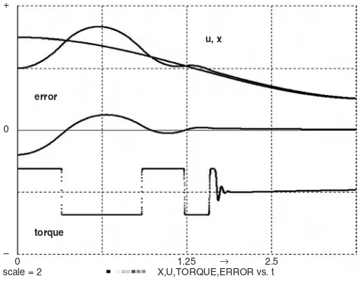
1-14. An Electrical Servomechanism with Motor Field Delay and Saturation

The motor of an electrical servomechanism drives a load so that the output displacementx follows a given input u = u(t), typically after an initial tran-sient (Fig. 1-8). The servo controller produces the motor-control voltage volt-ageas a function of the measured position error error = x – uand the rate of change xdot = dx/dtcontinuously measured by a tachometer on the motor shaft.

Figure 1-8 shows a simulation program. The sinusoidal servo input u = A * cos(w * t)reduces to a step input for w = 0. We model a simple linear controller with

voltage = – k * error – r * xdot (1-5)

Some nonlinear controllers will be discussed in Chapter 7. The controller gainkand damping coefficient rare positive controller parameters. As is well known, high gain and/or low damping speed the servo response but can cause output overshoot or even oscillations and instability.

The motor voltage (1-5) produces a field current I with a field-buildup delay modeled with

d/dt I = – B * I + g1 * voltage (1-6)

The resulting motor torque is limited by motor-field saturation modeled with the soft-limiting hyperbolic-tangent function:

torque = maxtrq * tanh(g2 * I/maxtrq) (1-7)

(42)

Control-system Examples 23

+

0

–

0 1.25 2.5

scale = 2 X,U,TORQUE,ERROR vs. t

u, x

error

torque

→

FIGURE 1-8. Complete simulation program and stripchart display for an electrical servo with motor-field delay, field saturation, and sinusoidal input u = A * cos(w * t). You can also setw = 0to obtain the step response of the servomechanism.

SERVOMECHANISM SIMULATION ---scale = 2 | display N1 | display C8 | -- display TMAX = 2.5 | DT = 0.0001 | NN = 10000

---A = 0.1 | w = 1.2 | -- --- signal parameters B = 100 | maxtrq = 1.5 | -- motor parameters g1 = 10000 | g2 = 1 | R = 0.6

k = 40 | r = 2 | -- -- controllerparameters

--drun

---DYNAMIC

---u = A * cos(w * t) | -- inp---ut

error = x - u | -- servo error

---voltage = - k * error - r * xdot | -- motor ---voltage

d/dt I = - B * I + g1 * voltage | -- motor field delay torque = maxtrq * tanh(g2 * V/maxtrq)

d/dt x = xdot | d/dt xdot = torque-R * xdot

--- scaled stripchart display X = 5 * x + 0.5 * scale | U = 5 * (u + scale)

(43)

The response of motor, gears, and load to the torque satisfies the differen-tial equations of motion

d/dt x = xdot

d/dt xdot = (torque – R * xdot)/M (1-8)

whereMrepresents the inertia of motor, gears, and load, and R > 0is a motor damping parameter. For convenience,torqueandRare scaled so thatM = 1.

The simulation program in Figure 1-8 sets system parameters and models the servomechanism with two defined-variable assignments (1-5) and (1-8) and three state differential equations (1-6) and (1-9). Control-system designers can then exercise the resulting “live mathematical model” to observe servo input, output, error, and motor torque while they adjust controller parameters and motor characteristics. Desirable parameter combinations must, in some sense, produce small servo errors. We can use different test inputs u(t) similar to inputs for the intended application, for example, step inputs, ramps, sinusoids (or noise, as in Section 5-8). Simulations must be repeated with different input amplitudes, since the field saturation makes our model nonlinear.

Such computer-aided experiments provide some intuitive feel for the control problem and may quickly indicate instability or design errors. For objective deci-sion-making, though, we must define and compute numerical error measures. These are typically functionals determined by the entire time history of the servo errorx(t) – u(t)for a given input u(t). One can, for instance, record the maximum of the absolute error or the squared error, as in Section 2-16c. More commonly used error measures are integrals over the error time history. We define such measures as extra state variables with zero initial values, for instance,

d/dt IAE = abs(x – u) (IAE, integral absolute error)

d/dt ISE = (x – u)2 _{(ISE, integral squared error)} d/dt ITAE = t * abs(x – u)

d/dt ISTAE = t2* abs(x – u)

whereISE/TMAXis the mean squared error.

We can now vary the design parameters until selected error measures meet acceptance limits, or until an error measure is as small as possible. We may also want to study our control system’s effect on the controlled system, for example, with a view to minimizing excessive space-vehicle accelerations. Parameter-influence studies are discussed in more detail in Sections 4-1 to 4-3.

1-15. Control-system Frequency Response

(44)

Control-system Examples 25 can instead simulate the system impulse response and program an ment-protocol script to produce its Fourier transform [9]. DESIRE experi-ment-protocol scripts can perform fast Fourier transforms and work with complex numbers for frequency-response and root-locus plots [9]. The book CD shows a number of simple examples.

1-16. Simulation of a Simple Guided Missile

(a) A Guided Torpedo

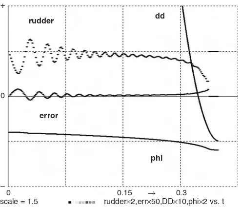
Figure 1-9ashows a missile pursuing a target [19–22]. The problem is scaled so that TMAX = 1, and distances are in 1000-foot units. xandyare rectangu-lar Cartesian coordinates of the missile center of gravity. uandvare velocity components along and perpendicular to the torpedo longitudinal axis. phiis the flight path angle, and rudderis the control-surface deflection. The target proceeds on a straight course at constant velocity.

Our particular missile will be a guided torpedo. In water, drag and side forces are approximately proportional to the square u2_of _{u. The accelerations along} and perpendicular to the torpedo’s longitudinal axis are then approximated by

(d/dt) u = (thrust – drag)/mass = UT a2 * u2

(d/dt) v = b1 * u2sinγ2 + b2 * u * phidot + b3 * v * rudder

The yaw-rotation equations are

(d/dt) phi = phidot

(d/dt) phidot = c1 * u2_{* sin}_γ_{+ c2 * u * phidot + c3 * u}2_{* rudder}

wherec1andc2are hydrodynamic- and damping-moment coefficients, and c3 is the rudder steering-moment coefficient, all divided by the torpedo moment of inertia.

Weathercock stability ensures that the angle of attack g2between longitu-dinal axis and velocity vector is so small that

sinγ ≈tanγ2≈v/u

and the equations of motion for our DYNAMIC program segment become

(d/dt) u = UT – a2_{* u}2

(d/dt) v = u * (b1 * v + b2 * phidot + b3 * rudder) (d/dt) phidot = u * (c1 * v + c2 * phidot + c3 * rudder) (d/dt) phi = phidot

(45)

The target angle psiis the angle between the horizontal line in Figure 1-9a

and a line joining the torpedo and target. The target coordinates xt, yt, the squared distance-to-target dd, and the target anglepsiare given by

xt = xt0 + vxt * t yt = yt0 + vyt * t

psi = arctan((yt – y)/(xt – x)) dd = (x – xt)2 _{+ (y – yt)}2

We aim the torpedo at the target by making the initial value of phiequal to psi. The initial values of uandvare set to 0.

We control the rudder to keep the torpedo turned toward the target. Such simple pursuit guidance works only for low target speeds unless initially one is 26 Introduction to Dynamic-system Simulation

Longitudinal axis

Velocity

phi u

γ2 v

+

0

–

–1.0 –0.5 0.0 0.5

target track

torpedo track

1.0 scale = 2 x,y,xt,yt

FIGURE 1-9a. A guided torpedo tracking a constant-speed target. The target angle psi, not shown here, is the angle between the horizontal line and the line joining the torpedo and target.

+

rudder

error

phi dd

0

–

0 0.15 → 0.3

scale = 1.5 rudder×2,err×40,dd×10,phi×2 vs. t

FIGURE 1-9b. Time histories of the torpedo rudder deflection, the error phi-psi, the angle

(46)

Control-system Examples 27

-- GUIDED-TORPEDO SIMULATION

-- (x, y) is torpedo, (xt, yt) is target

---irule 4 | ERMAX = 0.1 | -- variable-step RK4

---UC = 8 | -- torpedo parameters

a1 = 0.8155 | a2 = 0.8155 UT = a1 * UC^2

b1 = - 15.701 | b2 = - 0.23229 | b3 = 0 c1 = - 303.801 | c2 = - 44.866 | c3 = 500

---gain = 300 | rumax = 0.25 | -- control parameters

RR = 0.01 | rr = RR^2 | -- distance to target

DD = 100 * rr

---vxt = 0.1 | vyt = - 0.5 | -- target velocity vector

x = - 2 | y = 0 | -- initial values

xt0 = 1 | yt0 = 2 rudder = 0

phi = atan2(yt0 - y, xt0 - x) | -- first aim at target drunr

DYNAMIC

---xt = ---xt0 + v---xt * t | yt = yt0 + vyt * t | -- target

psi = atan2(yt - y, xt - x) | -- target angle

dd = (x - xt)^2 + (y - yt)^2 | -- squared distance

---d/dt u = UT - a2 * u^2 | -- state equations

d/dt v = u * (b1 * v + b2 * phidot + b3 * rudder) d/dt phidot = u * (c1 * v + c2 * phidot + c3 * rudder) d/dt phi = phidot

d/dt x = u * cos(phi) - v * sin(phi) d/dt y = u * sin(phi) + v * cos(phi)

--error = (phi-psi) | -- control

step | -- this is needed for sat()

rudder = - rumax * sat(gain * error)

--term rr - dd | -- terminate when close

---DISPXY x, y, xt, yt | -- draw 2 xy plots

(47)

more or less directly behind the target (Fig. 1-10). More advanced guidance systems are discussed in Reference [18].

Simple sonar guidance senses psiandddand actuates the control-surface deflectionrudderto implement

error = (phi – psi) rudder = – rumax * sat(gain*error)

We shall increase the controller gain as the torpedo approaches the target by setting

gain = gain0 + A * t

We terminate the run when the torpedo gets close to the target, where psi tends to change rapidly. The second equation ensures that the absolute value of the control-surface deflection does not exceed rumax.

(b) The Complete Simulation Program

Figure 1-9clists the complete guided-torpedo program used to produce the displays in Figures 1-9aandb. The experiment protocol first selects an inte-gration routine, display colors, and display scale, and then sets the initial value of the integration step DT, the simulation runtime TMAX, and the num-berNNof display sampling points.

The experiment-protocol script next sets torpedo parameters, initial target coordinates, and target-velocity components. Finally, we specify initial val-ues for the state variables x,y, and phi. The initial values of the remaining state variables u,v, and phidotare allowed to default to zero.

28 Introduction to Dynamic-system Simulation

+

0

–

+

0

– –1.0

scale = 1.5 x,y,xt,yt scale = 1.5 x,y,xt,yt

–0.5 0.0

(a) (b)

0.5 1.0 –1.0 –0.5 0.0 0.5 1.0

(48)

The DYNAMIC program segment following the DYNAMICline begins with the defined-variable assignments. We specify the target coordinates xt, yt as functions of time and then derive the target angle psiand the controller variables errorandrudder. The DYNAMIC segment next lists the state differential equa-tions and a termination command

term rr – dd

which stops the simulation when the missile closes to within RR = sqrt(rr). If it does not, our shot has failed, and the run continues to t = TMAX. The simu-lated rudder deflection rudderis bounded between – rumaxandrumaxwith the limiter function sat()(Section 2-8a), which follows a stepstatement to ensure correct integration (Section 2-11).

Finally, the display command DISPXY x, y, xt, ytcalls for simultaneous displays of the missile and target trajectories (yversus xandytversus xt). Alternative display statements can plot time histories of phi, psi, error, andrudder(Fig. 1-9b). The simulation program can be loaded from a file or an editor window. Solution displays will then appear when a run command is typed.

WHAT DO WE DO WITH ALL THIS?

1-17. Simulation Studies in the Real World: A Word of Caution

Simulations such as our torpedo example provide some insight and are nice for teaching and learning. But engineering-design simulation requires much more than solving textbook problems. In fact, the main result of a few model runs will be questions rather than answers: one begins to see how much more there is to know.Here are just a few questions that might come up:

• Can the missile acquire the target from different directions? • What happens if the target speed increases?

• Can the design be improved with different vehicle or control-system parameters?

• What parameter-value tolerances are acceptable?

We shall clearly require multirun simulation studies. Figure 1-10 shows a simple example, but in practice we shall have to investigate combinations of problems such as those listed. It follows that even a simple problem such as our torpedo can require over a thousand simulation runs. A larger project can generate an enormous volume of simulation data. Intelligent and efficient

(49)

evaluation of such results is an art rather than a science. It is the specific pur-pose of this book to show techniques that generate thousands of experiments in minutes and display results in various ways.

Computer simulation is convenient, and dramatically cheaper than real experiments. But engineering-design models are meaningless unless they can be validated by actual physical experiments. Very expensive prototype failures have been traced to oversimplified models (neglecting, for instance, missile fuselage bending or fuel sloshing). Simulation studies try to anticipate design problems and select test conditions that will minimize the number of expensive tests.

REFERENCES

1. U. M. Asher and L. Petzold, Computer Methods for Ordinary Differential Equations and Differential-Algebraic Equations, SIAM Press, New York, 1998. 2. H. Elmquist,Dymola User’s Manual, DynaSim A.B., Lund, Sweden, 2004. 3. L. Petzold, A Description of DASSL, a Differential-Algebraic-Equation Solver, in

Scientific Computing(R. S. Stepleman, ed.), North Holland, Amsterdam, 1989. 4. J. Stoer, et al. Introduction to Numerical Analysis, Springer, New York, 2002 5. G. A. Korn and J. V. Wait, Digital Continuous-System Simulation,

Prentice-Hall, Englewood Cliffs, NJ, 1978.

6. M. M. Tiller, Introduction to Physical Modeling with Modelica, Kluwer Academic Publishers (now Springer), New York, 2004.

7. P. Fritzon, Principles of Object-Oriented Modeling and Simulation with Modelica 2.1, Wiley, New York, 2004.

8. DYMOLA Manual, Dynasim A.B., Lund, Sweden, 2005.

9. G. A. Korn,Interactive Dynamic System Simulation with Microsoft Windows, Taylor and Francis, London, 1998.

10. F. Cellier and E. Kofman, Continuous-System Simulation, Springer, New York, 2006.

11. C. W. Gear, DIFSUB, Algorithm 407,Communications in ACM,14, No.

Advanced Dynamic system Simulation Free ebook download