Jitsuyōteki sōgo ketsugōmō no tame no rironteki sekkei hōhōron

(1)

Theoretical Design Methodology for

Practical Interconnection Networks

Ryota Yasudo

A dissertation submitted in partial fulfillment of the requirements for the degree of

Doctor of Philosophy

School of Science for Open and Environmental Systems Graduate School of Science and Technology

Keio University

(2)

(3)

Abstract

End-to-end network latency is a concern for parallel applications in high-performance computing platforms and high-end data centers. On one hand, computer architects have tried to design intercon-nection networks experimentally and empirically. On the other hand, theorists have tried to model computer networks and then studied their properties theoretically. However, the model does not suﬃciently capture real computer systems. This dissertation aims at establishing a novel method for designing high-performance network topologies to bridge a gap between the theoretical and practical studies. In particular, we make use of the knowledge of graph theory, network science, and design theory, as well as the research on interconnection networks.

We firstly present a novel graph called a host-switch graph, which consists of host vertices and switch vertices with maximum degree 1 andr, respectively. This graph represents a network topology of a practical parallel/distributed computer system with host computers connected byr-port switches. We then discuss important metrics for designing high-performance interconnection networks: the host-to-host average shortest path length (h-ASPL) and the bisection width (BiW). In particular, we explore a method for constructing host-switch graphs with low h-ASPL and high BiW that connect the fixed number of hosts via any number ofr-port switches. We demonstrate that the number of switches that provides the minimum h-ASPL can mathematically be approximated, and the minimum number of switches that provides a certain BiW can experimentally be approximated. On the basis of the approximations, we propose a randomized algorithm for searching host-switch graphs. We then apply the graphs to interconnection networks and compare them with typical network topologies. As compared with the torus, Dragonfly, and Fat-tree, our networks attain higher performance and smaller power and costs.

Furthermore, we propose adding ports to a host as a method for reducing the network latency as well as increasing the number of ports of a switch. To this end, we extend a host-switch graph so that it represents multi-port hosts. Multi-port hosts are conventionally used for link aggregation (LA) and network duplication (ND), but they do not reduce the hop count. We hence propose the permutation of host-switch mapping for reducing the hop count. It can be applied to LA and ND, and we label the obtained networks p-LA and p-ND, respectively. In addition, we propose the application of a finite projective plane (an instance of block designs) and label it PP. Our methods can be applied to arbitrary topologies, and thus we can directly use any existing topologies. We evaluate five designs above (LA, ND, p-LA, p-ND, and PP) for randomly-optimized, torus, Dragonfly, and Fat-tree topologies in terms

(4)

of the design complexity, the hop count, the bisection width, costs, the size of routing tables, and simulated message passing interface (MPI) performance. Our results demonstrate that our methods (p-LA, p-ND, and PP) reduce the hop count while increasing the bisection width and costs for every topology. In particular, we demonstrate that PP is a cost-eﬀective method for reducing the hop count, especially for randomly optimized and Fat-tree topologies.

(5)

Acknowledgments

First and foremost, I would like to thank my academic adviser, Professor Hideharu Amano, for his tremendous commitment to teaching and mentoring throughout my career as a graduate student.

I would like to thank Associate Professor Michihiro Koibuchi for his teaching and mentoring since I became a research assistant at National Institute of Informatics.

I would also like to thank Professor Tadao Nakamura, Professor Koji Nakano, and Associate Professor Hiroki Matsutani. I was fortunate to have them as teachers and collaborators, and my scientific perspective broadened.

I would also like to thank Professor Wayne Luk and Dr. Jose Gabriel de Figueiredo Coutinho for their tremendous supports when I was visiting Imperial College London, as well as collaborative research on reconfigurable computing.

I am grateful to my doctoral committee members, Professor Koji Nakano, Professor Katsuhiro Ota, and Associate Professor Hiroki Matsutani for their careful reviews and valuable comments to my thesis.

Last but not least, I would like to thank my family and friends for their supports and encouragement during my time at Keio University.

Ryota Yasudo Yokohama, Japan December 2018

(6)

(7)

List of Tables

3.1 Summary of fundamental properties of host-switch graphs. . . 41 3.2 Summary of nine topologies to connect more than 1024 hosts for simulation. . . 44 4.1 Time complexity for Step 1 (calculating ASPL between switches in a switch network)

and Step 2 (calculating h-ASPL between hosts on the basis of the results of Step 1). . 63 4.2 Total size of routing tables. . . 70 4.3 Improvement rate of simulated MPI performance relative to the case whenp= 1(%). 71

(12)

(13)

List of Figures

2.1 Concept of theoretical studies of network topology. . . 6

2.2 A conceptual figure of Dragonfly. . . 8

2.3 A conceptual figure of a multi-stage interconnection network. . . 8

2.4 An example of Fat-tree. . . 9

2.5 Concept of the use of network science for designing computer architecture. Network scientists mathematically model real-world networks, and then computer architects can apply the models for designing computer networks. . . 16

3.1 An example of a host-switch graph (n= 15, m= 4, r= 6). . . 22

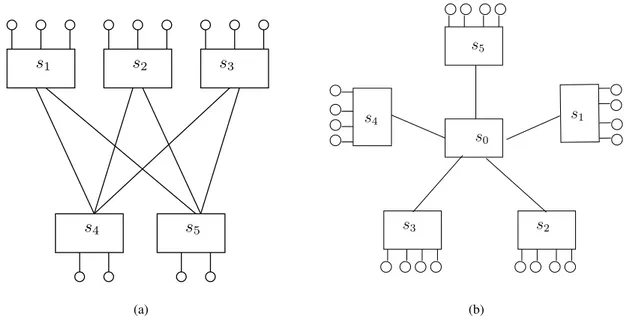
3.2 Examples of a biclique host-switch graph withr = 5; (a){m1, m2}={3,2},n= 13 and (b) star host-switch graph withn= 20. . . 26

3.3 An example of an XY-clique host-switch graph. . . 27

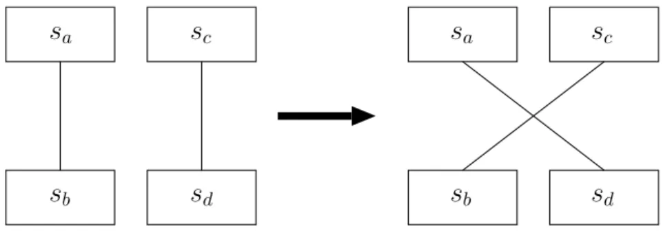
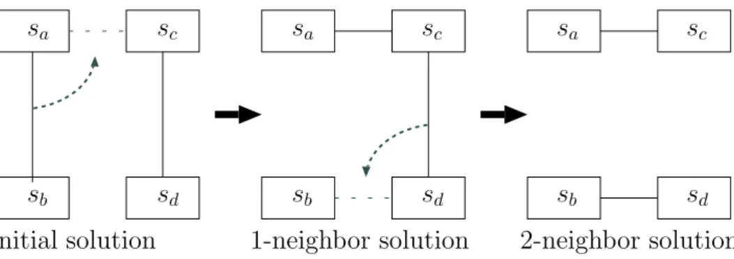
3.4 Swap operation which changes endpoints of two switch-switch edges. . . 31

3.5 Swing operation which changes endpoints of a switch-switch edge and a host-switch one. . . 31

3.6 2-neighbor swing operation (hosts are omitted for simplicity). . . 32

3.7 Relationship between h-ASPL and the number of switches. . . 33

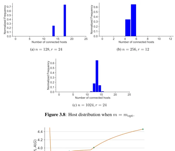
3.8 Host distribution whenm=mopt. . . 34

3.9 Comparison between the Moore bound and the continuous Moore bound. . . 34

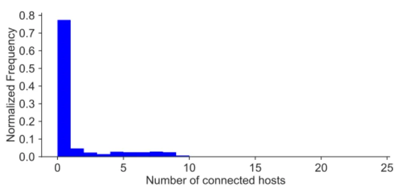
3.10 Host distribution of a host-switch graph with unused switches when (n, m, r) = (1024,1024,24). . . 35

3.11 Changes of h-ASPL and BiW during optimization. . . 36

3.12 Relationship between the BiW and the number of switches. . . 37

3.13 Results of comparisons between torus and proposed topology: (a) Performance (eight benchmarks and the geometric mean); (b) Power consumption; (c) Cost breakdown (Cable and Switch); (d) Performance per watt. . . 46

3.14 Results of comparisons between dragonfly and proposed topology: (a) Performance (eight benchmarks and the geometric mean); (b) Power consumption; (c) Cost break-down (Cable and Switch); (d) Performance per watt. . . 47

(14)

3.15 Results of comparisons between fat-tree and proposed topology: (a) Performance (six benchmarks and the geometric mean); (b) Power consumption; (c) Cost breakdown (Cable and Switch); (d) Performance per watt. . . 48 4.1 An example of a host-switch graph with 6 2-port hosts and 4 5-port hosts. . . 54 4.2 Conventional interconnection networks with multi-port hosts whenp= 2. (a) Link

Aggregation (LA). (b) Network Duplication (ND). . . 55 4.3 Proposed methods whenp = 2. (a) Permutation for Link Aggregation (p-LA). (b)

Permutation for Network Duplication (p-ND). . . 57 4.4 Obvious design represented by Euclidean plane. (a)p= 2. (b)p= 3. . . 59 4.5 Proposed design applying a finite projective plane and its incidence graph (p = 3).

(a) The Fano plane. (b) The incidence graph of the Fano plane, where a line and a point of the Fano plane correspond to a host-group and a switch network, respectively. 60 4.6 Hop count of randomly optimized topologies withp-port hosts (0 ⩽ p ⩽6) when

(n, r) = (1024,16)and(n, r) = (10000,32): (a) h-ASPL and (b) diameter. . . 64 4.7 Hop count of torus topologies withp-port hosts (0 ⩽ p ⩽ 6) when n ⩾1024and

n⩾10000: (a) h-ASPL and (b) diameter. . . 65 4.8 Hop count of Dragonfly topologies withp-port hosts (0 ⩽ p ⩽6) whenn ⩾1024

andn⩾ 10000: (a) h-ASPL; (b) diameter; and (c) radix. Note that the Dragonfly changes radix according to the required number of connected hosts. . . 66 4.9 Hop count of Fat-tree topologies withp-port hosts (0⩽p⩽6) whenn⩾1024and

n⩾10000: (a) h-ASPL; (b) diameter; and (c) radix. Note that the fat-tree changes radix according to the required number of connected hosts. . . 67 4.10 Bisection widths. The line denoted by “100%” shows full bisection width, i.e.,n/2. . 68 4.11 Costs of cable and switches when n ⩾ 1024: (a) Randomly optimized topologies;

(b) Torus topologies; (c) Dragonfly topologies; and (d) Fat-tree topologies. Note that the number of hosts is not fixed; costs per host is shown in Fig. 4.12. . . 69 4.12 Costs per host of cable and switches when n ⩾ 1024: (a) Randomly optimized

(15)

List of Theorems

2.1 Problem (Degree/Diameter Problem) . . . 13

2.2 Problem (Order/Degree Problem) . . . 15

3.1 Lemma (Trivial upper bound on the order) . . . 22

3.1 Theorem (Upper bound on the order) . . . 23

3.1 Corollary (Lower bound on the diameter) . . . 23

3.2 Theorem (Lower bound on the h-ASPL) . . . 24

3.1 Problem (Radix/Diameter Problem) . . . 25

3.3 Theorem (Upper bound on the order of a host switch graph of diameter 2) . . . 25

3.2 Lemma (Condition for constructing a host-switch graph of diameter 3) . . . 25

3.4 Theorem (Upper bound on the order of a host-switch graph of diameter 3) . . . 25

3.3 Lemma (Upper bound on the switch order of a biclique host-switch graph) . . . 26

3.5 Theorem (Upper bound on the order of a biclique host-switch graph) . . . 27

3.4 Lemma (Conditions for constructing an XY-clique host-switch graph) . . . 27

3.6 Theorem (Upper bound on the order of an XY-clique host-switch graph) . . . 28

3.7 Theorem (The order of an XY-clique and star host-switch graphs) . . . 28

3.5 Lemma (Upper bound on the order of a polarity host-switch graph) . . . 28

3.2 Problem (Order/Radix Problem) . . . 30

3.1 Observation (Relationship between the h-ASPL and the continuous Moore bound) . . 34

3.2 Observation (Relationship between the h-ASPL and the BiW) . . . 36

3.3 Observation (Linear relation between the number of switches and the BiW) . . . 37

4.1 Definition (LA) . . . 56

4.2 Definition (ND) . . . 56

4.1 Lemma (Upper bound on the diameter of a network with multi-port hosts) . . . 60

A.1 Lemma . . . 77

A.1 Corollary . . . 77

(16)

(17)

Chapter 1 Introduction

1.1 Motivation

The international roadmap for devices and systems (IRDS 2017 edition [7]) predicts that a cloud system is one of the important market drivers. Cloud systems support many important applications such as web service, multimedia, shopping, big data analytics, and high-performance scientific computation. In particular, big data analytics is increasingly important with the growth of big data for social networking, artificial intelligence (AI), smart cities, and so forth. Big data requires abundant computing power and continuing performance scaling.

A typical application of big data analytics is used as the Graph 500 benchmark [4]. In the Graph 500 benchmark, graph construction and breadth-first search (BFS) are processed. BFS requires many communications as compared with computation. Furthermore, the communications have few locality. To accelerate the Graph 500 benchmark, reducing costs of data movement is therefore essential.

As with big data applications including the Graph 500 benchmark, data-intensive applications such as physical system simulation are also emerging. In general, Peter Kogge suggests that we are now facing the locality wall on the heels of the memory wall and the power wall; growing non-predictable regularity and non-locality limits the performance [2]. To accelerate such applications, we need to improve the latency and the bandwidth for both memory and interconnection networks. Especially, interconnection networks should provide faster all-to-all communication and support irregular communication patterns. Thus, irregular network topology that handles non-local traﬃc would work eﬀectively.

1.2 Objectives

A long-standing design goal for high-performance computing (HPC) is to provide low end-to-end network latencies between compute nodes. This requirement for low latency is also relevant for high-end data center networks (DCN). For example, DCNs that target high-frequency trading (HFT)

(18)

applications can benefit from end-to-end latencies down to microseconds levels, thus motivating the use of interconnects traditionally used in HPC platforms.

Supporting large-scale applications requires large-scale platforms, e.g., exascale platforms that aggregate millions of cores in hundreds of thousands of compute nodes. Large-scale HPC platforms are currently deployed as compute nodes that are interconnected using large numbers of switches, and DCNs are built following a hierarchical structure with so-called top of rack (ToR) switches, cluster routers, and border routers [9]. In both cases, end-to-end network paths between two compute nodes traverse multiple switches located in diﬀerent cabinets. End-to-end latencies must decrease to design scalable platforms for workloads that lead to many small message exchanges between compute nodes. Especially, switch delays are high as compared with wire and flit injection delays; for instance, port-to-port switch latency reaches 90 nanoseconds in InfiniBand EDR 100 Gb/s switch [6]. Thus, the number of switches traversed by a network path, called thehop count, should be reduced.

Recent research shows that complex networks such as small-world and random networks have low hop counts. Moreover, such complex networks should provide fast all-to-all communications and support irregular traﬃc patterns, and thus they satisfy the requirement of data-intensive applications, described in Section 1.1. Therefore, this dissertations study a design method and practical feasibility of complex network topologies with low hop count.

1.3 Contributions

To achieve the objectives above, this dissertation mainly makes the following contributions.

1. We survey both theoretical and practical studies for graphs, complex networks, and inter-connection networks, including graph theory, network science, design theory, and computer engineering.

2. We propose a novel graph called a host-switch graph. It will firstly be defined as a model of an interconnection network with single-port hosts, and then extended to a model of an interconnection network with multi-port hosts.

3. We establish two novel graph problems: theradix/diameter problem(RDP) and theorder/radix

problem(ORP). Subsequently, we provide some theory and solutions for both problems.

4. We propose and run a heuristic algorithm for solving ORP. It is based on the simulated annealing, but it includes a new concept called a2-swingoperation and acontinuous Moore bound. 5. For interconnection networks with multi-port hosts, we propose two novel methods for reducing

the network latency: permutation of host-switch mappingand application of finite projective planes.

(19)

1.4. Dissertation Outline 3 6. We compare our proposed network topologies with existing network topologies including theoretically proposed topologies and practical topologies used in supercomputers ranked in TOP500.

1.4 Dissertation Outline

The rest of this dissertation is organized as follows.

Chapter 2 describes technical and theoretical backgrounds. Technical backgrounds include ar-chitectural concepts of interconnection networks for large-scale parallel computer systems from three perspectives: the topology, the routing, and the layout. Theoretical backgrounds include graph theory, design theory, and network science; the study set forth in this dissertation eﬀectively applies them to practical interconnection networks.

Chapter 3 studies low-latency interconnection networks with single-port hosts. The two novel concepts are proposed: a host-switch graph and the order/degree problem. A host-switch graph is a model of an interconnection networks with hosts and switches, and the order/degree problem is a graph problem for minimizing the ideal (zero-load) end-to-end latency of an interconnection network. Several interesting findings are described.

Chapter 4 studies low-latency interconnection networks with multi-port hosts. To represent a network with multi-port hosts, a host-switch graph is extended. As in Chapter 3, the ideal end-to-end latency is minimized. To this end, the solution obtained in Chapter 3 can be utilized. It is shown that design theory provides excellent design of the networks with multi-port hosts.

(20)

(21)

Chapter 2 Technical and Theoretical Backgrounds

2.1 Interconnection Networks

Aninterconnection networkis a programmable system that transports data between terminals [39]. It occurs at many scales, including on-chip networks (a.k.a. networks-on-chip) and oﬀ-chip networks. Physical characteristics depend on the scale, but fundamental principles are the same. In this section, we describe interconnection networks with a focus on oﬀ-chip ones.

Three issues mainly dominate the design of an interconnection network: topology, switching technique, and routing algorithm. In addition to the three issues above, this section studies the physical layout, which is becoming more and more important due to the increasing gap between switching delays and cable delays.

2.1.1 Topology

2.1.1.1 Theoretical Studies on Network Topology

Theoretically, a topology of a computer network is represented as an undirected graph, in which vertices and edges correspond to computers and communication links, respectively. The performance potentiality of the network can be measured by analyzing topological properties of the graph. In the design of networks for computer systems such as multiprocessors and supercomputers, there are certain requirements and limitations. In particular, requirements include the number of nodes, and limitations include the degree and the diameter. Hence the three parameters above have been studied in graph theory. The degree/diameter problem (DDP) is a classical problem for such studies. The DDP is the problem of finding the largest number of vertices in a graph of given maximum degree∆

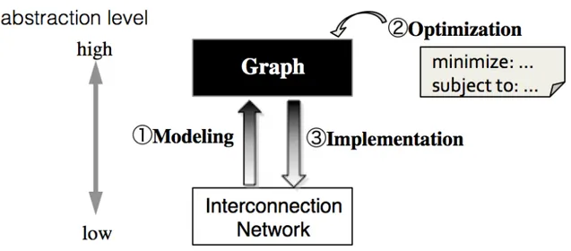
and diameterD. The known upper bound—called the Moore bound [86]—on the number of vertices of an undirected graph is 1 + ∆∑D_i₌₀−1(∆−1)i. Near-optimal/optimal solutions of the DDP are considered for topologies of interconnection networks [21, 77, 87]. Figure 2.1 illustrates a concept of theoretical studies of network topology.

(22)

Figure 2.1: Concept of theoretical studies of network topology.

However, the DDP solutions may not be usable for building network topologies in practical interconnection networks. This is because the DDP requires the specific number of vertices, and hence we cannot meet technical requirements such as the number of nodes. To cover this shortcoming, we should fix the number of vertices (order) of a graph. We can consider the order/degree problem (ODP), the problem of finding the smallest diameter in a graph of given order and degree. Although less attention is given to the ODP as compared with the DDP, the ODP is recently studied by designers of interconnection networks [5].

In the field of network science, researchers find that complex networks such as social networks provide low diameter and ASPL. Thus some models are proposed, e.g, a cycle plus a random match-ing [28], the Erdős-Rényi model (random graph) [49], and the Watts-Strogatz model (small-world networks) [121]. Some solutions for the ODP are such complex graphs and applied to computer systems, including high-performance computing systems [76], data centers [110], and on-chip net-works [95]. To apply such complex topologies to practical netnet-works, physical layouts [74] and routing algorithms [55] are also studied.

Even if we tackle the ODP, however, a shortcoming remains; in conventional graph theory, one kind of vertex is considered on a graph, though two types of nodes—hosts and switches—exist in typical interconnection networks. Hence, the mapping between vertices and physical devices is not obvious. If we regard vertices as switches, we have no information for hosts. This is a serious issue because the mapping strongly aﬀects the network performance (we show this in Section 3.4). Therefore, we should radically change both a model of interconnection networks and a graph problem.

2.1.1.2 Practical Studies on Network Topology

Practical studies on topologies of interconnection networks for parallel/distributed computer systems have a long history. In the 1970s, hypercubes were used in many systems such as Cosmic Cube [106];

(23)

2.1. Interconnection Networks 7 in the 1980s, 2-D/3-D tori and meshes became the mainstream due to their short cables that provide high bandwidth and cost-eﬃciency; from the 1990s to 2000s, as the number of nodes becomes over 10 thousand, high-radix networks such as the dragonfly [71] are researched for reducing communication overhead; and now, in the 2010s, the high-radix networks are used in commercial high-performance computers [13, 15].

All the networks above aredirect networks, which denote the networks such that a certain number of hosts are connected to each switch. In addition to direct networks, indirect networksare also used, which denote the networks such that some switches are connected with a certain number of hosts while the other switches are connected with no hosts. Above all, the fat-tree [78] is widely used in parallel/distributed computer systems from generation to generation, though technology for each generation is diﬀerent (e.g., both CM-5 [63] in the 1980s and Tianhe-2 [81] in the 2010s use the fat-tree). In this respect, indirect networks contrast with direct networks. For this reason, the question of our interest is how we should uniformly discuss direct and indirect networks (note that prior theoretical study based on the DDP and the ODP deals with only direct networks). This should be studied systematically, but there has been no prior research to answer this question yet. Also, the rationality of existing topologies should be backed by graph theory.

2.1.1.3 Commonly Used Existing Topologies

Torus The torus topology is a mesh graph (a.k.a. a lattice graph or a grid graph) with wrap-around channels, and consequently each dimension constitutes a ring structure. Formally, aK-ary N-torus is a topology with parameters K and N. Each node is identified by a N-bit base-K addressaN−1aN−2· · ·a0, and connected to nodes with addressesa′_N₋₁a′_N₋₂· · ·a′0 where a′i±1

(modK) =aifor anyi(0⩽i⩽N −1) anda′j =aj for allj(0⩽j ⩽N−1andj̸=i).

Dragonfly Dragonfly is, so to speak, a meta-topology proposed for designing technology-driven, highly-scalable interconnection networks with high-radix routers [71]. It consists of multiplegroups, in which an intra-group network connect the routers, and an inter-group network as shown in Fig-ure 2.2. In [71], Kimet al. suggest that every intra-group network should be a clique or Flattened butterfly and the inter-group network should be a clique. However, rather interestingly, the topologies of inter- and intra-group networks are not deterministic since Dragonfly is not topology itself but a meta-topology. Also, we can change parameters such as the number of links within a group and between groups.

Dragonfly provides a high-performance networks, so it is adopted by many supercomputers ranked in Top 500.

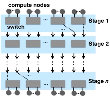
Fat-tree Fat-tree is a class ofbidirectional multi-stage interconnection networks(BMIN). MIN is a directed network consisting of multiple stages as shown in Figure 2.3; then, by folding it, we get an

(24)

…

compute nodes

switch

group

intra-group

network

…

compute nodes

switch

intra-group

network

inter-group network

…

Figure 2.2: A conceptual figure of Dragonfly.

… … … … … … … … … … … … … … … … … … … … …

Stage 1

Stage 2

Stage

_n

compute nodes

switch

Figure 2.3: A conceptual figure of a multi-stage interconnection network.

undirected network, i.e., BMIN. An example of Fat-tree is shown in Figure 2.4. In this figure, Fat-tree has three layers—called core, aggregation, and edge layers—and it provides full bisection bandwidth.

2.1.1.4 Bridging a Gap between Theoretical and Practical Studies

The study set forth in this dissertation aims at establishing a novel method for designing high-performance network topologies to bridge a gap between theoretical studies based on graph theory and practical studies based on computer engineering. There exist many gaps between graphs and real systems; a real system may consist of various types of nodes, including CPUs, accelerators, memories, and switches, and we should consider the execution time for real applications, the fault tolerance, the layout, and the energy consumption.

(25)

2.1. Interconnection Networks 9 … … … … … … … …

…

… … … … … … … …

…

compute nodes switch Core layer Aggregation layer Edge layer

Figure 2.4: An example of Fat-tree.

This study focuses on distinguishing hosts and switches and considering the end-to-end latency between two hosts. We will present a novel graph called ahost-switch graph, which consists ofhost

vertices andswitchvertices. A host can be connected to exactly one switch using an edge. A switch can be connected to at mostr vertices, each of which is a host or a switch. Clearly, a host-switch graph represents a topology of a computer network with 1-port host computers andr-port network switches. Thus, studying the topological characteristics of host-switch graphs leads to find good topologies for practical computer systems.

2.1.2 Routing 2.1.2.1 Switch

Large-scale HPC platforms are currently deployed as compute nodes that are interconnected using large numbers of switches, and DCNs are built following a hierarchical structure with so-called top of rack (ToR) switches, cluster routers, and border routers [9]. In both cases, end-to-end network paths between two compute nodes traverse multiple switches located in diﬀerent cabinets. End-to-end latencies must decrease to design scalable platforms for workloads that lead to many small message exchanges between compute nodes. Especially, switch delays are high as compared with wire and flit injection delays; for instance, port-to-port switch latency reaches 100 nanoseconds in InfiniBand QDR [6]. Thus, the number of switches traversed by a network path, called the hop count, should be reduced.

To reduce the hop count, switches with dozens of ports, called high-radix switches, have been used in the HPC domain for many years [72, 104]. High-radix switches expand the design space for topologies because a variety of high-degree topologies become feasible. It is thus possible to use network topologies with the low diameter and the low average shortest path length (ASPL) [21, 56, 67, 71, 77, 87], both measured in the hop count. Recently, random [76, 110] (or randomly optimized [90, 124]) topologies are demonstrated to provide the ASPL and the diameter that are close to the lower bounds [90, 124]. However, switch complexity increases quadratically impacting

(26)

on the area, costs, and the latency in a switch. Thus, the number of ports of a switch is limited, and low-radix switches are preferred if the hop count is the same [123].

2.1.2.2 Routing Algorithm

A switch determines a route (a proper output port) for each incoming packet so that it finally reaches the destination node. In general, thisroutingmust guaranteedeadlock-freedomandlivelock-freedom.

A deadlockrefers to a situation such that group of agents (packets) are unable to act because of

waiting each other to release some resource (buﬀers or channels). Alivelockrefers to a situation such that packets are unable to reach their destinations although they can continue to move. Obviously, a livelock occurs only if non-minimal routing is used. A livelock can easily be avoided by specifying one or more paths for every pair of nodes and bounding the number of misroutings. However, how to design deadlock-free routing is not clear.

For regular topologies, specific deadlock-free routing algorithms can be designed and used; for example, dimension-order routing for two-dimensional mesh topologies. However, for irregular topologies, there exist no specific routing algorithm, and hence we need a general method to de-sign deadlock-free routing algorithm for arbitrary topologies. We now describe previous work that proposes such methods and theoretical foundations on deadlock-free routing.

Dally’s theory Dally et al. introduces a channel dependency graph (CDG) for guaranteeing deadlock-freedom of arbitrary interconnection networks [38]. ACDG, for a given interconnection network and a given set of possible routing paths, is a directed graph where

• the vertices denote the channels of the interconnection network;

• the edges denote the possible routing paths.

Dallyet al. then proved that an interconnection network is deadlock-free if and only if the CDG is acyclic (we call itDally’s theory). Note that Dally’s theory per se is not routing algorithm. Also, Dally’s theory allows us only to check whether given pair of a network and routing is deadlock-free or not.

Turn model and its extensions Theturn model[59] is a well-known application of Dally’s theory for two-dimensional mesh/torus topologies. In the turn model, the packet forwardings are divided into four directions: north, south, east, and west. The change of directions, called aturn, are then classified into eight patterns; note that all the turns make right angles. As a result, we can see there exist only two types of cyclic dependencies (clockwise and counterclockwise). Thus, a deadlock-free routing can be designed by prohibiting one turn for each type of cyclic dependency.

The turn model, however, restricts the topology to mesh and tori. Thus, the turn model has been extended ton-dimensional topologies without diagonal links [45] and arbitrary topologies [69].

(27)

2.1. Interconnection Networks 11 Using additional buﬀers Virtual channels are also useful for avoiding deadlock on the basis of Dally’s theory. Thelayered shortest path(LASH) [113] uses virtual channels to achieve deadlock-free minimal routing. LASH can be combined with thetransition oriented routing(TOR) [102] to enable flexibility of the diﬀerent algorithms among the virtual channel layers; it is calledLASH-TOR[112].

In-transit buﬀers(ITB) also enable a deadlock-free minimal routing. Packets are ejected from the network temporarily and stored in an ITB when deadlock occurs. These methods can be applied to arbitrary network topology and use the shortest path routing. Thus, we can assume the shortest path routing for any topology.

Up*/Down* routing Up*/Down* routing, introduced in [103], is a deadlock-free routing method that avoids cyclic dependencies by using spanning trees obtained by using a breadth-first search. Given network topology, a spanning tree is constructed and the packet forwardings are classified into theup direction or thedowndirection; then, a routing is deadlock-free if there exist no move to the up direction after moves to the down direction. A drawback of the Up*/Down* routing is the poor performance due to the biased link utilization.

Several methods for improving Up*/Down* routing have been proposed. Sanchoet al. demon-strated that using a depth-first search (DFS) instead of BFS when constructing a spanning tree improves traﬃc balance [100]. Left-up-first turn routing(L-turn routing) [75] improves Up*/Down* routing by usingL-R directed-graph, which is a transformation of the spanning tree and has left and right directions in addition to up and down directions. Using this graph, it distributes prohibited turns (in particular, avoids the heavy traﬃc around the root node of the spanning tree), and consequently the throughput is improved.

2.1.3 Layout

The nodes of an interconnection network are typically arranged in two-dimensional space. The layout determines the lengths of cables, and consequently it is essential for reducing signal propagation delay and cabling costs. Large-scale computer systems such as supercomputers have historically used Manhattan cabling in floorplan, because Euclid cabling makes both cabling and its maintenance become complex due to the diagonal cables on a floor. In the case of simple networks such as 2-D mesh networks, the layout is easily determined. However, in the case of irregular networks studied in this dissertation, the layout is not clear. Thus, we focus on the layout of irregular network topologies.

2.1.3.1 Quadratic Assignment Problem

The layout of an interconnection network is determined by mapping each cluster to a cabinet on a floorplan so that the total cable length becomes minimum. This problem corresponds to the facility location problem, which has been studied in operation research [52]. This problem is NP-hard, and thus there is no known algorithm for solving this problem in polynomial time. Hence,

(28)

metaheuristics-based techniques have been developed to solve it. Solutions to this problem have been used in the computer industry for computer chip design and physical network layouts for HPC systems.

When we determine physical network layouts, we should reduce the cable lengths (the maximum length or the average length or both); this should be formulated as a quadratic assignment problem (QAP). It is reported that several algorithms can successfully applied to QAP (e.g., the simulated annealing [35], the robust tabu search [117], the reactive tabu search [20], the greedy random-ized adaptive search procedure [96], the fast ant colony algorithm (FANT) [116], and the memetic algorithm [84].

2.1.3.2 Randomly Optimized Grid Graph

Nakano et al. propose a method for designing interconnection networks with link-length con-straints [90] by introducing a new graph called agrid graph. Using this, they propose a randomized algorithm for optimizing network topologies and layouts at the same time. Agrid graphis a graph G = (V, E) such that V = {(x, y) | 0 ⩽ x, y ⩽ √N −1} is a set ofN nodes and E is a set of edges connecting a pair of two distinct nodes inV. We can think that nodes in V are arranged in a 2-dimensional space so that each node(x, y) is located at position (x, y). Letl(u, v) denote the Manhattan distance of two nodesuandv inV, that is, l(u, v) = |ux−vx|+|uy −vy|, where

u = (ux, uy) andv = (vx, vy). In a network with topology represented by a grid graph, the two nodes(u, v)are connected by a communication link of lengthl(u, v)wired along the grid.

A grid graphG = (V, E)isL-restricted ifl(u, v) ⩽L for all edges(u, v) ∈ E. Clearly, in a network with topology represented by anL-restricted grid graph, the length of every communication link is restricted to no more thanL. A grid graph isK-regularif every node is connected withK edges. In [90], the authors show lower bounds on the diameter and the average shortest path length (ASPL) ofK-regularL-restricted grid graph and provide aK-regularL-restricted grid graph whose diameter and ASPL are close to the lower bounds by using a randomized algorithm.

Moreover, [90] discusses quite interesting relationship betweenN,K, andL; the authors derive the following asymptotic formula, which provides awell-balanced1grid graph:

Θ(logN/logK) ≈ Θ(√N /L). (2.1)

Let us here describe an interesting finding. From (2.1), we have a decreasing functionlogK = Θ(LlogN/√N)ofN. Thus, ifLis fixed andN is increased,K must be decreased to keep well-balanced. Quite surprisingly, this relationship suggests that we should reduce the number of ports in each node of a computer system when we increase the number of nodes, provided that we use communication cables with the same technology.

1AK-regularL-restricted grid graph iswell-balancedif the absolute diﬀerence between the lower bound on the ASPL

(29)

2.2. An Undirected Graph 13 Nakaharaet al. extended a grid graph so that it represents a 3D-NoC and call it astacked grid

graph [89]. They proposed a method for optimizing the average shortest path length and energy

consumption of a 3D-NoC by using a multi-objective simulated annealing (MOSA) [92].

2.2 An Undirected Graph

2.2.1 Definition and Notation

Anundirected graphis an ordered pairG= (V, E)where

• V is a set of elements calledvertices, and

• Eis a set of elements called edges, each of which is a 2-element subset ofV.

In the field of computer architecture, an undirected graph is used to represent a network of a computer system. An undirected graph is preferred to a directed graph because an interconnection networks use bi-directional links rather than uni-directinal ones.

There are three parameters important for interconnection networks: the number nof vertices (called theorder), the maximum number of edges connected to a vertex∆(called thedegree), and the maximum value of the shortest path lengthD (called the diameter). The shortest path length ℓ(u, v)is the smallest possible path length between two vertices,uandv. The order should increase so that many processing units operate in parallel to improve the performance. The degree should be limited because designing a switch with many ports require high costs and the switching latency. The diameter should be reduced as much as possible because the ideal2 communication latency depends on the path length between a source and a destination; the diameter is especially important for reducing the worst case communication latency.

In this context, thedegree/diameter problem(DDP) has traditionally been attracting attention. This problem is defined as follows.

Problem 2.1(Degree/Diameter Problem). Given natural numbers∆andD, find the largest possible

ordernin an undirected graph with maximum degree∆and diameterD.

The DDP is considered for several classes of graphs, including undirected graphs, directed graphs, mixed graphs, bipartite graphs, planar graphs, and so forth. Among them, this dissertation focuses on the cases of undirected graphs, which are used for representing interconnection networks, and bipartite undirected graphs, which we will use in Chapter 4.

2.2.2 Degree/Diameter Problem for General Graphs

Let us consider the tight upper bound on the ordern+of an undirected graphG= (V, E)with degree

∆and diameterD. Trivially, if∆ = 1, thenD= 1andn+= 2. Hence, we assume that∆⩾2.

(30)

For any fixed vertex u ∈ V, we can partition all the vertices inV into subsetsV0, V1, . . . such

thatVi ={v∈V |ℓ(u, v) =i}. Clearly,V0 ={u}and|V0|= 1hold. Sinceuis connected with at

most∆edges,|V1|⩽∆holds. Since each vertex inV1 is connected with at most∆−1vertices in

V2,|V2|⩽∆(∆−1)holds. In general, we have

|Vi|⩽    1 ifi= 0 ∆(∆−1)i−1 _if_i_⩾₁ . (2.2)

Thus, the upper bound on the order of an undirected graph with degree∆and diameterDbecomes as follows: n+ = 1 + D ∑ i=1 ∆(∆−1)i−1 (2.3) =    1 + ∆(∆−_∆1)₋D₂−1 if∆>2 2D+ 1 if∆ = 2 . (2.4)

This upper bound is called theMoore bound, and a graph of ordern+is called aMoore graph[64]. Solutions of DDP are applied to topologies of interconnection networks. For example, MMS graphs [83] are applied to Slim Fly [21].

2.2.3 Degree/Diameter Problem for Bipartite Graphs Abipartite graph(a.k.a. bigraph) is a graphG= (V1, V2, E)where

• V1andV2are two disjoint and independent sets of vertices, and

• Eis a set of edges that connect a vertex inV1to one inV2.

A bipartite graph is said to bebiregularif two vertices in the same bipartition class have the same degree. We can consider DDP limited to the bipartite graphs.

The tight upper bound on the ordern+_biof a bipartite graph with maximum degree∆and diameter Dwas given by Biggs [24]:

n+_bi =    2(∆−1)D₋₁ ∆−2 if∆>2 2D if∆ = 2 . (2.5)

This upper bound is called thebipartite Moore bound, and a bipartite graph of ordern+_biis called a

bipartite Moore graph.

Ageneralized polygonis a biregular bipartite graph such that the girth is equal to2D. Feit and Higman proved that a∆-regular finite generalized polygon (i.e., a bipartite Moore graph) with∆>2

is either a complete bipartite graph (D= 2), a finite projective plane (D = 3), a finite generalized quadrangle (D= 4), or a finite generalized hexagon (D= 6) [53]. Chapter 4 will apply this theorem for designing interconnection networks.

(31)

2.2. An Undirected Graph 15 2.2.4 Order/Degree Problem

Even though DDP solutions have been applied to topologies of interconnection networks, they may not directly be usable for network topologies in supercomputer and data center systems. This is because they are for particular number of vertices (corresponding to compute nodes in a system), whereas the number of nodes in a real system is determined based on practical considerations such as power consumption and costs.

In this context, researchers on computer engineering proposed another graph problem called the

order/degree problem(ORP) [5].

Problem 2.2(Order/Degree Problem). Given natural numbernand∆, find the minimum possible

diameterDin an undirected graph with order nand maximum degree∆. If two or more graphs

take the minimum diameter, find the minimum possible average shortest path length (ASPL) in an undirected graph with the minimum diameter.

Note that, by definition, ORP contains two objective functions: the diameter and the ASPL.

Let us consider the tight lower bounds on the diameterD−and the ASPLA− of an undirected graphG= (V, E)with ordernand maximum degree∆. For any fixed vertexu∈V, we can partition all the vertices inV intoV0, V1, . . .such thatVi = {v ∈ V |ℓ(u, v) =i}. Clearly,V0 ={u}and

|V0|= 1hold. Sinceuis connected with at most∆edges,|V1|⩽∆holds. Since each vertex in|V1|

is connected with at most∆−1vertices inV2,|V2|⩽∆(∆−1)holds. In general, we have

|Vi|⩽    1 ifi= 0 ∆(∆−1)i−1 ifi⩾1 . (2.6)

From Eq. 2.4, we have

D=    log_∆₋₁ ( (n+₋_1)(∆₋₂₎ ∆ + 1 ) if ∆>2 n+−1 2 if ∆ = 2 . (2.7) Thus, we have D− =    ⌈ log_∆₋₁ ( (n−1)(∆−2) ∆ + 1 )⌉ if ∆>2 ⌈_n₋₁ 2 ⌉ if ∆ = 2 . (2.8)

Letm(i)be theMoore functionsuch that

m(i) =    1 ifi= 0 min ( 1 +∑i_j₌₁∆(∆−1)j−1, n ) ifi⩾1 . (2.9)

Clearly, the number of vertices reachable inihops fromudoes not exceedm(i). Thus, we have A−=∑

i⩾1

(m(i)−m(i−1))·i

(32)

Figure 2.5: Concept of the use of network science for designing computer architecture. Network scientists mathematically model real-world networks, and then computer architects can apply the models for designing computer networks.

2.3 Network Science and its Applications

Thus far, we have described (classical) graph theory and examples of mathematical problems and results. What we have shown in this dissertation is just a tip of an iceberg, and there exists much beautiful and elegant work in the field of graph theory. However, several researchers in various fields such as complex systems, sociology, biology, and computer engineering should understand properties of real-world networks, which are possibly complex, dynamic, and/or stochastic. Thus, the new science of networks callednetwork sciencehas been studied empirically as well as theoretically. Mainly, researchers have proposed three basic models of real-world networks, which we describe below. Computer architects utilize network science for designing computer architecture on the basis of the concept shown in Fig. 2.5.

2.3.1 Random Graph Models

Arandom graph—introduced by Solomonoﬀ and Rapoport [114] and studied extensively by Erdős

and Rényi [49, 50]—is a graph obtained by randomly sampling from a collection of possible graphs with fixed number of vertices. Among several proposed models, theErdős-Rényi model, described below, is mostly be studied.

The Erdős-Rényi (ER) model generates a random graphGn,pas follows: 1. Fix the numbernof vertices and probabilityp(0< p <1).

2. Connect each pair of vertices with independent probabilityp.

As a result, the ER model generates either of possible2n(n−1)/2graphs, including a complete graph and a graph with no edge. However, it is known thatpdetermines the properties of ER model. For example, the ER model almost surely provides a connected graph whenp⩾logn/nwhile it does not whenp <logn/n. Such a qualitative change according to the value ofpis called aphase transition.

According to [27], the average distanceLsatisfies L≈ logn

(33)

2.3. Network Science and its Applications 17 where⟨k⟩denotes the average degree. Thus, when we use a random graph for the network topology, the ASPL becomesO(logn), which grows slowly as the order increases. That is why using randomness when constructing network topologies is helpful for designing low-latency interconnection networks. The random graphGn,phas a specific degree distribution. Since each vertex is connected to the othern−1vertices with probabilityp, the degree distribution becomes

p(k) = (n−1)! k!(n−1−k)!p

k₍₁₋_p₎n−1−k_, _(2.12)

wherep(k)denotes the probability that the degree of a vertex isk. It is clearly a binomial distribution and becomes the Poisson distribution in the limit wheren→ ∞,p →0, and(n−1)p →λ(λis a positive constant).

Computer architects may think that the degree distribution should not be the Poisson distribution. Instead, a network should be regular, i.e., the degree is fixed. To construct a random network with arbitrary degree distribution, we can use an extended model of random graphs. Theconfiguration model[93] generates a random graph with arbitrary degree distribution as follows:

1. Fix the numbernof vertices.

2. Fix the degree distributionp(0), p(1), . . . , p(kmax)wherekmaxdenotes the maximum degree

(kmax⩽n−1).

3. Generate thedegree sequencek1, k2, . . . knso that it satisfies the fixed degree distribution. 4. Generate a random graphG= (V, E)whereV ={v1, v2, . . . vn}and the degree ofviiski.

According to [93], the average distanceLof a configuration model satisfies the following if⟨k2⟩ exists in the limit wheren→ ∞:

L= 1 + log

n ⟨k⟩

log⟨k2_⟨⟩−⟨_k_⟩k⟩

. (2.13)

One of the important examples of the configuration model is aregular random graph. It is a random graph where the degree of all the vertices is the same, i.e.,⟨k⟩. Thus, it is straightforward to use a regular random graph for a topology of an interconnection network since the network typically consists of the switches with fixed ports. Several researchers propose the use of a regular random graph for designing network topologies [51, 74, 90, 109, 110, 123, 124].

2.3.2 Watts-Strogatz Model

In 1967, Milgram demonstrated thesmall-world phenomenon, that is to say, human society consists of a network with short path-lengths; more specifically, people in the United States seemed to be connected by approximately three friendship links on average, without speculating on global linkages [85]. This phenomenon is sometimes associated with the phrase “six degrees of separation” and regarded as a characteristics of real-world complex networks.

(34)

Afterward, in 1998, Wattz and Strogatz published an epoch-making paper proposing the

Wattz-Strogatz (WS) model(a.k.a. the small-world model), which excellently characterizes the networks

with the small-world phenomenon [121]. The WS model provides a network with the short average distance and the largeclustering coeﬃcient, which denotes the probability that two adjacent nodes of a node is connected.

The WS model provides a network as follows:

1. Fix the numbernof vertices and the average degree⟨k⟩(⟨k⟩is an even number). 2. Construct a cycle graph withnvertices.

3. Connect a vertexuand the vertices that can be reached within⟨k⟩/2hops fromu. 4. Change an endpoint of an edge with independent probabilityp(0⩽p⩽1).

Obviously, the obtained network depends on the value ofp. When p = 0, a network becomes an extended cycle graph. Whenp= 1, a network almost corresponds to a random graph obtained by the ER model. The small-world phenomenon is obtained whenp ∈ [0.01,0.1]. The degree of the WS model is fixed whenp= 0, and its distribution approaches the Poisson distribution aspincreases.

According to [19], the clustering coeﬃcientC(p)of the WS model with probabilitypsatisfies C(p) = 3⟨k⟩ −6

4⟨k⟩ −4(1−p)

3_. _(2.14)

According to [94], the average distanceL(p)of the WS model with probabilitypsatisfies L(p) = 2n ⟨k⟩f ( n⟨k⟩p 2 ) , (2.15) f(x) = 1 2√x2_{+ 2}_xtanh −1 ( x √ x2_{+ 2}_x ) . (2.16)

Note thatL(p) is minimized whenp = 1. Hence we should use the ER model rather than the WS model if we consider only the ASPL of a network topology. However, the clustering coeﬃcient decreases aspincreases.

Several researchers propose the use of a small-world network for designing network topologies [41, 95, 108]

2.3.3 Models of Scale-free Networks

One might wonder if the models described above capture real-world networks precisely. In fact, they do not. In 1999, Albert et al. showed that the power law described the topology of the World-Wide Web [14]. Formally, the degree distributionp(k)satisfies

(35)

2.4. Design Theory 19 A random graph with the power law degree distribution is called ascale-free network. There are many models describing the scale-free networks. For example, the configuration model, described earlier, is one of such models.

Cohen and Havlin [34] shew that the average distance L (or the diameter) of the scale-free networks satisfies L∝    log logn if2< γ <3 logn/log logn ifγ = 3.

(2.18)

Note that the average distance grows more slowly asnincreases than it does in the case of small-world networks. Thus, Cohen and Havlin say that scale-free networks areultra-small.

Several researchers propose the use of a scale-free network for designing network topologies [54, 62]. However, a scale-free network would not be useful for designing interconnection networks because it requires switches with many ports, which should induce high switching latency and costs. Also, the number of ports of a switch do not vary.

2.4 Design Theory

In combinatorial mathematics, design theory [43] refers to the study ofdesigns—systems of finite sets whose arrangements satisfy generalized concepts of balance or symmetry or both. In particular, it studies necessary and suﬃcient conditions for the existence of ablock design.

Ablock designwith parameters(v, b, r, k, λ)is a pair(X,A)where

• Xis a set ofvelements (calledpoints),

• Ais a family ofbsubsets ofX, each of cardinalityk(calledblocks),

• Every point occurs in exactlyrblocks, and

• Every pair of distinct points occurs in exactlyλblocks.

IfA ={X}, then(X,A)is obviously a block design, and it is said to be anobviousdesign. Also, ifAis a set of the k-subsets ofX, then(X,A) is obviously a block design, and it is said to be a

completedesign. If a block design is neither obvious nor complete, it is called abalanced incomplete block design(BIBD) and denoted as(v, b, r, k, λ)-BIBD. The five parameters are not all independent; the basic two equations are

bk = vr, (2.19)

λ(v−1) = r(k−1). (2.20)

Thus, it is not uncommon to write a BIBD as a(v, k, λ)-BIBD.

The most basic necessary condition for the existence of a BIBD known asFischer’s inequality, named after the statistician Ronald Fisher, states that a(v, b, r, k, λ)-BIBD exists only ifb ⩾ v(or

(36)

equivalently, ifr⩾k). A BIBD withb=v(or equivalently,r=k) is called asymmetricBIBD. The parameters of a symmetric design satisfy

λ(v−1) =k(k−1). (2.21)

Finite projective planes are symmetric BIBD withλ= 1. From Eq. 2.21, finite projective planes satisfy

v−1 =k(k−1). (2.22)

Sincer =kholds by the definition of a symmetric BIBD, the ordernof a finite projective plane is equal tok−1. From Eq. 2.22, we obtainv= (n+ 1)n+ 1 =n2+n+ 1points in a finite projective plane of ordern. Thus, a finite projective plane of ordernis a(n2+n+ 1, n+ 1,1)-BIBD.

From a (v, b, r, k, λ)-BIBD, we can construct a graph called an incidence graph (a.k.a. Levi graph), which is a bipartite graphG= (V1, V2, E)where

• V1is a set of points,

• V2is a set of blocks, and

• Eis a set of edges that connect a pointpiand a blockBjif and only ifpi occurs inBj. The incidence graph of a BIBD will be applied to a network topology in Chapter 4.

(37)

Chapter 3 Low-Latency Interconnection Networks with

Single-Port Hosts

3.1 Overview

In this chapter, we deal with two topological properties that are important for designing interconnection networks, the host-to-host average shortest path length (h-ASPL) and the bisection width (BiW). We propose a method for designing a topology with low h-ASPL and high BiW. By analyzing host-switch graphs, we provide answers to the following questions: (1)given the number of hosts and the number of ports per switch, how many switches should be used?; and (2)which is better, direct or indirect networks, in terms of the h-ASPL and the BiW?

First, Section 3.2 provides theoretical foundation of host-switch graphs; we formally define a host-switch graph and provide upper and lower bounds on the maximum number of hosts, the diameter, and the h-ASPL. Second, Sections 3.3-3.4 present host-switch graphs with low h-ASPL; we take deterministic and heuristic approaches in each section. Here we demonstrate that the heuristic approach is more practical than the deterministic one for certain reasons. We empirically show that the optimal number of switches is a key parameter for host-switch graphs in terms of the h-ASPL and also the BiW. Third, in Section 3.5, we practically compare proposed network topologies with existing ones in terms of performance, topological properties, power consumption, and cost breakdowns. Section 3.6 reviews related work, and finally, we conclude the chapter in Section 3.7.

3.2 Introduction of a Host-Switch Graph

3.2.1 Definition and Notation

₇

Figure 3.1: An example of a host-switch graph (n= 15, m= 4, r= 6).

• S={s0, s1, . . . , sm−1}is a set ofmelements calledswitch vertices(or simplyswitches), and

• E⊂ {{si, sj} |si, sj ∈S} ∪ {{hi, sj} | (hi ∈H)∧(sj ∈S)}is a set of unordered pairs of connected vertices callededges.

The numbernof hosts is called theorderofG. Each host must be connected with exactly one edge while each switch is connected with at mostredges. Thus each switch must have at leastrports. The numberrof required ports per switch is called theradixofG. In Fig. 3.1 we illustrate an example of a host-switch graph with 15 hosts and 4 switches with radixr = 6. Throughout this paper, a circle and a rectangle represent a host and a switch, respectively.

Clearly, at leastm−1edges are necessary to connectmswitches such that they are reachable each other. Sincemswitches can connect at mostmredges, we can state:

Lemma 3.1(Trivial upper bound on the order). For any connected host-switch graph withm r-port switches, the ordernis not greater thanmr−2(m−1).

For any two hostshi and hj, let ℓ(hi, hj) denote the number of edges along the shortest path betweenhi andhj. For example, ℓ(h0, h14)of a host-switch graph shown in Fig. 3.1 is 4, because

the shortest path between them is(h0, s0, s1, s3, h14). Usingℓ(hi, hj), we can define two topological properties. ThediameterD(G)of a host-switch graph is defined as

D(G) := max{ℓ(hi, hj)|0⩽i < j < n}. Thehost-to-host average shortest path length (h-ASPL)A(G)is defined as

A(G) := ∑ 0⩽i<j<n ℓ(hi, hj)/ ( n 2 ) .

(39)

3.2. Introduction of a Host-Switch Graph 23 These metrics are essentially diﬀerent from the diameter and the average shortest path length (ASPL) of an ordinary undirected graph in that the considered path is between hosts rather than switches. In this paper we mainly discuss the h-ASPL, because it measures the ideal all-to-all communication latency of interconnection networks.

3.2.2 Upper and Lower Bounds

Let us consider tight upper bound on the order of a host-switch graph with r and D(G). For any source host hs ∈ H, we can partition all the hosts in H into subsets H0, H1, . . . such that

Hi = {hd ∈ H | ℓ(hs, hd) = i}. Similarly, we can partition all the switches in S into subsets

S1, S2, . . .such thatSi ={sd∈S |ℓ(hs, sd) =i}. LetAhs(G)andDhs(G)respectively denote a

single-source h-ASPL fromhsand a single-source diameter fromhs, as follows:

Ahs(G) :=

∑

0⩽i<n,i̸=s

ℓ(hs, hi)/(n−1),

Dhs(G) := max{ℓ(hs, hi)|0⩽i < nandi̸=s}.

Using these notations, we obtain the upper bound on the order, as follows:

Theorem 3.1 (Upper bound on the order). For any host-switch graph with radix r and diameter

D(G), the ordernof a host-switch graph is not greater than(r−1)D(G)−1+ 1.

Proof. For any fixed hosthsof a host-switch graph, letNibe the upper bound on|Hi|+|Si|. Clearly,

Niis equal to          |H0|= 1, ifi= 0 |S1|= 1, ifi= 1 |Si−1|(r−1). ifi >1 (3.1)

Hence, to maximize the order, we must satisfy Ni = |Si|for 1 ⩽ i < D(G) andNi = |Hi|for

i=D(G). In this situation, the order is D_∑(G)

i=0

|Hi|= (r−1)D(G)−1+ 1.

The lower bound on the diameter follows from Theorem 3.1:

Corollary 3.1(Lower bound on the diameter). For any host-switch graph with ordernand radixr, the diameter is not less than⌈log_r₋₁(n−1)⌉+ 1.

Let us call a host-switch graph with a root hosthsand(r−1)Dhs(G)−1leaf hosts afull host-switch tree. Clearly, the lower bound onAhs(G)is the lower bound onA(G).

Jitsuyōteki sōgo ketsugōmō no tame no rironteki sekkei hōhōron

Theoretical Design Methodology for

Practical Interconnection Networks

Ryota Yasudo

Abstract

Acknowledgments

Contents

List of Tables

List of Figures

List of Theorems

Chapter 1

Introduction

1.1

Motivation

1.2

Objectives

1.3

Contributions

1.4

Dissertation Outline

Chapter 2

Technical and Theoretical Backgrounds

2.1

Interconnection Networks

…

…

…

compute nodes

switch

group

intra-group

network

…

…

…

compute nodes

switch

intra-group

network

inter-group network

…

Stage 1

Stage 2

Stage

n

compute nodes

switch

…

…

2.2

An Undirected Graph

2.3

Network Science and its Applications

2.4

Design Theory

Chapter 3

Low-Latency Interconnection Networks with

Single-Port Hosts

3.1

Overview

3.2

Introduction of a Host-Switch Graph

h

h

h

h

h

h

h

h

h

h

h

h

h

s

s

s

s

h

_n