Musen tsushin shisutemu ni okeru kansho moderuka, kanri, kaihi ni kansuru kenkyu

- ii -.

- iii -.

- iv -.

-v-.

- vi -.

- vii -.

- viii -.

- ix -.





𝐾.











,. 𝑁.

𝑠. 𝑎.

𝑞(𝑠, 𝑎) ← 𝑞(𝑠, 𝑎) + 𝜅(𝑟(𝑠, 𝑎) + 𝛾 max(𝑞(𝑠 ′ )) − 𝑞(𝑠, 𝑎)) 𝑠. 𝑠′. 𝑎. 𝜅. 𝛾 𝑁× 𝑀 𝑀. 𝜀. 𝜀. 𝑁.























. . . . . . .

Interference Phenomena. Interference Avoidance/Manag ement in CR Networks. Interference Modeling/Management in Heterogeneous Cellular Networks. Cognitive Cellular Networks. Reliable Communications. Optimal ChannelSensing Scheme. Machine-learning. Interference Alignment (IA)/Management in Multi-User MIMO Interference Channels. Stochastic Geometry. Rayleigh Fading Assumption. Closed-form Outage Probability Expressions Nakagami-m Fading. Chapter 2. Chapter 4. Tight Closedform Outage Probability Expressions. Iterative IA Based Transceiver Designs. Power Allocation. Chapter 5 Chapter 3.

Interference Avoidance/Manag ement in CR Networks. Reliable Communications. Licensed Spectrum Sensing. Wavelet Detection [12]. Matched Filter [9]. A Cognitive Engine (CE). Covariance Detection [13] Cyclostationary Detection [11] Licensed Spectrum Management/Control. Energy Detection [10]. Markov Decision Process (MDP) [19] Partially Observable MDP (POMDP). Unsupervised Learnings [22], [23], [24]. Reinforcement Learning (RL) [17], [18]. Fuzzy Qlearning (FQL). Chapter 2. Q-learning (QL) [24]. Learning Based Techniques. Supervised Learnings [20], [21]. Support Vector Machines (SVMs) [20].

Interference Modeling/Management in Heterogeneous Cellular Networks Traditional Macrocells Deployment Rapid Increase of User Population. Increased Capacity Demand and Cost Challenges Traffic Offloading Spots to Decrease the Congestion in Macrocells Development of the Existing Cellular Infrastructure [29]. Heterogeneous (Multi-tier) Cellular Networks Frequency-Reuse across the Coexisting Tiers [32] Cognitive Heterogeneous Cellular Networks. Low-Powered/Cost Small Cells [30], [31]. Picocells Microcells. Increased Interference Interference Management. Interference Modeling. Interference Evaluation Metrics. Rayleigh Fading Assumption. Outage Probability. Chapter 3 Chapter 4. Femtocells. Traditional Hexagonal Grid Model [33] Stochastic Geometry [34], [36]. Nakagami-m Fading.

Interference Alignment (IA)/Management in Multi-User MIMO Interference Channels Interference: a Major limiting Factor in Achieving Reliable Communications. Interference Management Schemes. Interference Alignment (IA). IA in Time Domain [44]. IA in Space Domain [46]. IA in Frequency Domain [45]. MIMO Networks. Availability of Global and Perfect CSI at Nodes [51], [52]. Availability of Local CSI at Nodes-CSI Estimation Step is Applied. Orthogonal Access Schemes TDMA [43]. FDMA [42]. IA Solutions. Closed-form [53], [54] Iterative IA with Leakage Minimization [56]. Iterative IA Iterative IA with MaxSINR [56]. Equal Power Allocation Assumption [56], [57]. Chapter 5. Iterative IA with Sum-rate Maximization. Sum-rate Maximization Based Power Allocation.



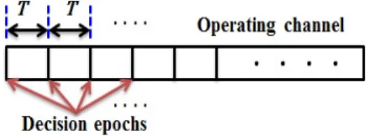
Chapter 2. Optimal Channel-Sensing Scheme for Cognitive Radio Systems Based on Fuzzy Q-Learning. 2.1 Introduction Energy detection is the most common approach to channel sensing [58]. is because of its low implementation complexity.. This. One of the main drawbacks of. energy detectors is that they need a large amount of data in order to be able to detect the signals at very low SNR values. This makes the sensing duration very long to guarantee sufficiently low detection error probability [59], [60]. Typically, in the periodic sensing strategy (where CR periodically senses the channel to monitor the PU activity) (e.g., [58], [61], and [62]), after each sensing period. 𝑇 , the energy detector. provides a real-valued test statistic as the result of energy detection. CR can make a hard decision on the state of the PU (active or not) by comparing this test statistic with a certain threshold. Thus, period. 𝑇. must be long enough that PU activity can be. reliably detected and the final decision of PU activity is correct. Since the CR is not allowed to transmit any data during a sensing period, a long sensing duration results in low channel utilization and QoS for the CR network. Moreover, according to [10], [61], and [63] in some environments, very short spectrum opportunities (spectrum holes). 25.

caused by fast PU state variations are available for the CR to exploit.. Therefore,. the CR should frequently perform channel sensing in much shorter time intervals to catch the fast variations in the PU state and consequently exploit these short spectrum opportunities. On the other hand, because of the short sensing period, it is difficult for the CR to make an accurate decision on the PU activity only from the single test statistic (provided by the energy detector) over the sensing result. Furthermore, since such sensing results are noisy, the CR has to combine multiple factors (i.e.. multiple sensing results) to provide reliable information regarding the. PU state after each sensing period and takes the test statistic into account only as a soft “sensing result.” Sequential decision-making is the cognitive process leading to the selection of actions among variations at consecutive decision epochs (see Fig.. 2.1).. One-way. to automate the decision making process is to provide a model of dynamics for the domain in which a machine will make decisions.. A reward structure can be used. to motivate immediate decision that will maximize the future reward.. The aim of. the decision-making algorithm is to maximize channel utilization for the CR while restricting interference to the PU. To design the optimal algorithm that achieves such goal, we use POMDP framework [64]. POMDP is an aid in the automated decisionmaking.. POMDP policy informs the CR what action to be executed.. It can be a. function or a mapping and typically depends upon the channel state. In summary, in each short sensing interval, the CR uses the energy detection method to obtain knowledge about PU state. However, the CR does not rely only on this knowledge and combines more soft sensing results to enhance adaptability and adaptive decisions at the sequential decision epochs are made by the optimal decision-making algorithm, which was designed by using the POMDP framework. Indeed, a POMDP is equivalent to a MDP with a continuous state space [65], [66]. In this chapter, we formulate the channel sensing in the CR network as a POMDP problem. This statistical-based sensing model uses a probabilistic, rather than deterministic approach to design the optimal decision-making algorithm. In the POMDP model decision, an agent (i.e.. CR) tries to maximize some reward function in the. 26.

face of limited and noisy information about its surrounding environment (i.e. PU). Although POMDP has emerged as a powerful framework for modeling and optimizing sequential decision making problems under uncertainty, achieving an optimal policy is computationally very challenging [65], [67]. As mentioned before, POMDP is equivalent to MDP with a continuous state space. 𝑏,. called belief state. Thus, a POMDP. policy is a mapping from a region in belief state space to an action. Not surprisingly this is extremely difficult to construct and whilst some works make use of POMDP framwork (e.g., [62], and [63]), they do not present solution algorithms for POMDP, or their solutions do not scale to problems with continuous state space and multi-agent domains. RL has now established itself as a major and powerful scheme to address adaptive optimal control of uncertain systems and learn the optimal policy [17]. On the other hand, fuzzy expert systems also have been extensively used in intelligent control problems where mostly traditional methods have poor performance. With the utilization of fuzzy theory in RL, we can enhance learning with more adaptation of RL for continuous and multi-agent domains and speedup learning process [26]. In this chapter, a FIS is also employed for generalizing a continuous belief space POMDP. We propose a FIS-based RL controller with a FQL implementation to solve the POMDP problem. FQL is an approach to learn a set of fuzzy rules by reinforcement. It is an extension of the popular QL algorithm [68]. Learning fuzzy-rules makes it possible to face problems where inputs are described by real-valued variables (continuous state spaces), matched by fuzzy sets. Fuzzy sets play the role of the ordinal values used in QL, thus making possible an analogous learning approach, but overcoming the limitations due to the interval-based approximation needed by QL to face the same type of problems. We will present the simulation results that show how the proposed scheme for channel sensing achieves significant performance in terms of channel utilization while restricting interference to the PU.. 27.

2.2 System Model 2.2.1 Model Description Consider a frequency channel that the PU is licensed to use.. The CR network. can access the channel whenever it is not occupied by the PU. A collision happens if the CR network sends data on the channel currently being used by the PU. We consider a small-scale network such as the wireless personal area network with a “master node (MN)” in its center and “slave nodes (SNs)” attached to the MN, and assume that all of them are adjusted to the same frequency channel, called “operating channel,”. It should be noted that we do not consider the PU activities on frequency channels other than the operating channel, because they are needed only for frequency channel selection, to which we do not pay attention in this chapter. The MN performs channel sensing on the operating channel when it is necessary (not periodically) and the channel sensing process is monitored only by the MN, whereas the SNs do not. If the PU is detected, then the MN switches the operating channel to another channel and directs the SNs to move to the new operating channel [63].. Clearly, based on. the sensing results, the MN chooses the next appropriate action at each decision epoch, and it informs the SNs from the chosen action by sending a control signal. As soon as receiving the control signal, the SNs follow the order in it. Indeed, the MN senses the operating channel and provides the SNs with information about the PU activity, while user data are exchanged only by the SNs. To see the fundamental performance of the proposed method and for simplicity of exposition, we ignore fading and shadowing. It should be noted that in real communication environments, fading and shadowing can deteriorate the spectrum sensing performance of the CR user and cause interference to the PU, consequently. To solve this problem, cooperative sensing method (multi-agent scenario) is usually introduced that can be considered as future work.. 2.2.2 System Structure As stated, the MN chooses the next proper action at each decision epoch, which occurs at the end of each action. The decision epoch is indexed by. 28. 𝑡(= 1, · · · ).. The.

Fig. 2.1. A CR can make channel-sensing decisions over short time intervals. MN selects the appropriate action among “data transmission”, “stop data transmission”, and “channel switching”. In Section 2.3, we explain how this action is selected by the MN. In the following we explain the operating modes of the CR network when each decision is made by the MN.. 1) Data Transmission: whenever the MN is convinced that the operating channel is not occupied by the PU, it selects data transmission for the SNs. The SNs will be aware of the MN’s decision upon receiving the control signal sent by the MN. Then SNs immediately start to exchange user data by using the time-division multipleaccess (TDMA) approach.. The SNs perform data transmission during a period. 𝑇. (same as the sensing period for the MN) allocated by the MN in the received control signal. During this period the MN will be quiet.. 2) Stop Data Transmission: if the MN is not sure about the PU existence over the operating channel, then it prefers to select stop data transmission. This decision is clearly made to avoid from a probable collision with the PU. Similar to the case which the selected action by the MN is data transmission, a control signal containing the selected action and the allocated time interval is sent to the SNs, and thus the SNs stop data transmission as soon as receiving the control signal and the MN starts to do channel sensing for another. 𝑇. period.. 3) Channel Switching: when the MN realizes the PU existence with a high certainty, it selects channel switching and sends a control signal that orders the SNs to switch the operating channel. We assume that it takes. 𝑇𝑐. to complete the channel-. switching process and be ready to choose another action, since the CR nodes should tune their frequency band and perform a synchronization process.. 29.

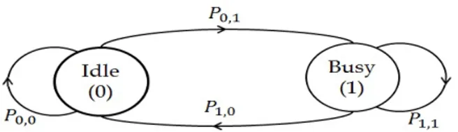
2.3 Decision-Making Configuration 2.3.1 POMDP Formulation In this section, we formulate the adaptive sensing, in the CR network as a POMDP to design the optimal decision-making algorithm.. A POMDP framework has been. investigated in [63], [64]. In [61], [62] it is shown that the PU activity can be modeled as a Markov process with two states as. 𝑠𝑡 ∈ {0, 1}. where. 𝑠𝑡. represents the state of. the operating channel (see Fig. 2.2). Empirical measurements taken in the 928-948 MHz paging band [69] and in 802.11b based wireless Local Area Network (WLAN) ([70], [71]) have also validated a Markovian pattern in the spectrum occupancy of the PU.. 𝑠𝑡. 𝑡th. is 0 if the operating channel is vacant at. operating channel is occupied by the PU at. 𝑡th. decision epoch and 1 if the. decision epoch.. However, the CR. network does not know the true state of the PU and only infers it from noisy sensing results.. In such environments where the CR network’s information about the PU. activity is incomplete, the theory of POMDP will be the best candidate for modeling the situation [64], [72].. To choose the appropriate action at each decision epoch,. “belief state” is calculated.. Belief state is a probability distribution over the PU. state, which is prepared by the MN. In [64], it is shown that the belief state contains all the necessary information for making an optimal decision. As depicted in Fig. 2.1, at each decision epoch having this belief state, the MN selects an action among the possible actions: data transmission, stop data transmission, and channel switching. The belief state at each decision epoch is denoted by probability of state. b𝑡 = (𝜋 0,𝑡 , 𝜋 1,𝑡 ), where 𝜋 𝑖,𝑡. 𝑖 ( 𝑖 ∈ {0, 1}) at 𝑡th decision epoch.. is the. Note that the MN performs. channel sensing (using energy detection method) on the operating channel during a period of which the length is probability. 𝑌𝑖,𝑒. MN receives. 𝑒. 𝑇. and presents its obtained result as the observation. in the belief state formula. We define. 𝑇. immediately after the. 30. as the probability that the. 𝑖.. The output of energy detector. 𝑡th. decision epoch is expressed as. as the observation in channel state. with the sensing period. 𝑌𝑖,𝑒.

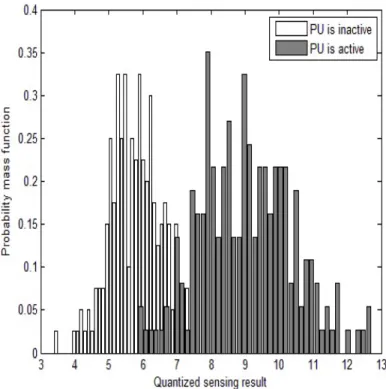
Fig. 2.2. The state-transition diagram of the PU follows:. 𝑊𝑇 1 ∑︁ |𝑦𝑗,𝑡 |2 𝐸𝑡 = 𝑁0 /2 𝑗=1. where. 𝑦𝑗,𝑡. denotes the. epoch, and. 𝑁0. (2.1). 𝑗 th signal sample in the sensing period 𝑇. after the 𝑡th decision. is the noise spectral density used for normalization and assumed to. be known from the MN viewpoint.. 𝑊. is the bandwidth of the frequency channel.. According to [10], [63] the sensing result obtained by the energy detection method follows the chi-square distribution with 2𝑊 𝑇 degrees of freedom if the PU is inactive. If the PU is active, then the sensing result follows the non-central chi-square distribution with the same degrees of freedom as that of the case that PU is inactive and the non-central parameter of 2𝑃 𝑇 /𝑁0 , where. 𝑃. is the power of the received PU. signal. Fig. 2.3 shows the probability mass functions (pmf ’s) of the simulation sensing results when the PU is inactive and active. Therefore, the observation probability denoted by. 𝑌𝑖,𝑒. can be easily calculated from the pmf ’s of the sensing results. Besides. the observation probability that is a soft sensing result, the other factor in the belief state formula is the state transition probability of the PU. Let be the state transition probability of the PU from state. 𝑖. 𝑃𝑖,𝑗 (𝑖, 𝑗 ∈ {0, 1}). to state. 𝑗.. We may first. assume that the MN is aware of the state transition probability as in [62] and [63]. In practice, this may not be achievable. The problem then becomes one of POMDP with unknown transition probability. In Section 2.5, we completely explain how the state transition probability of the PU is estimated. We also assume that the PU’s state can change only once during each. 𝑇. period.. From now on, we will explain how the belief state is calculated. As mentioned before, the belief state. b𝑡. is inferred by the MN at the. previous actions and observations. After the. 31. 𝑡th. 𝑡th. decision epoch on the basis of the. decision epoch, the decision-making.

b𝑡. algorithm updates. to. b𝑡+1. on the basis of the selected action at the. epoch and the received observation during the period. 𝑇. after the. 𝑡th. 𝑡th. decision. decision epoch.. If the selected action is data transmission, then the SNs exchange the user data for the. 𝑇. period and the MN will be quiet in this period and receives a null observation. (no sensing result).. In this case, the belief state formula evolves according to the. state transition probability. That is, the algorithm updates the belief state based on the assumed Markovian evolution as follows:. (︃. 1 ∑︁. 𝑃𝑖,0 𝜋 𝑖 ,. 𝑖=0. 1 ∑︁. )︃ 𝑃𝑖,1 𝜋 𝑖. .. (2.2). 𝑖=0. If the selected action is stop data transmission, then the SNs stop transmitting data for the. 𝑇. period, and the MN performs sensing (energy detection) during this. period. Therefore, besides the state transition, the sensing result of energy detection in the form of the observation probability is also taken into account by using Bayes’ theorem as follows:. (︃. 𝑌0,𝑒. ∑︀1. 𝑖 𝑌1,𝑒 𝑖=0 𝑃𝑖,0 𝜋 , 𝑓. 𝑓 = 𝑌0,𝑒. 1 ∑︁. 𝑖 𝑖=0 𝑃𝑖,1 𝜋 𝑓. 𝑃𝑖,0 𝜋 𝑖 + 𝑌1,𝑒. 𝑖=0. 𝜋 1,𝑡 ). 1 ∑︁. )︃. 𝑃𝑖,1 𝜋 𝑖 .. (2.3). (2.4). 𝑖=0. From (2.3) and (2.4) and Fig. the state of PU is 1 (i.e.,. ∑︀1. 2.3, we can see that for example, the belief that. increases as the quantized value of the sensing result. increases. This corresponds to the fact that a high value of the sensing result indicates a high probability that the channel is occupied (clearly, a low probability that the channel is idle). Thus, the soft sensing result (energy detection result) is well taken into account in updating the belief vector and has an important role in making the final decision. The goodness of the POMDP framework is that even in the case of a sensing error observed in the energy detection result, the decision making algorithm can still make a reliable decision (relying on the other soft sensing results) compared. 32.

to the case when this energy detection result is used as the only available information in making the final decision. However, it is clear that a better performance of the energy detection method, results in more accurate decisions for the CR. If the action is channel switching, then the CR network moves to the next channel. In this case, the probability distribution over the PU state (belief state) converges to the stationary probability. 𝜂.. The proposed approach is easily applicable to multi-agent POMDP. domains (with two or more MNs) wherein each MN maintains a belief simultaneously and communicates it to a central FIS (it can be via communication by wire) at each decision epoch, which forms a fuzzy mapping of the belief space of the underlying multi-agent POMDP. This fuzzy belief mapping is then used to solve a sequence of Bayesian games to generate an approximate optimal joint policy which is executed by each agent (i.e.. MN). Under this joint action, each MN updates his own belief. and the whole system receives a signal that indicates the goodness of executing the joint action (joint reward). This signal is then used to tune q-values to reflect the consequence of taking that joint action as per standard QL.. 2.3.2 Solution to POMDP We define the total discounted reward of the MN as sidered as the reward of the MN at. 𝑡th. ∑︀∞. 𝑡=1. decision epoch and. 𝛾 𝑡 𝑟𝑡 ,. where. 𝛾 ∈ (0, 1). 𝑟𝑡. is con-. is a discount. factor. In the discounted reward model, we are given a discount factor. 𝛾,. and the. goal is to maximize total discounted reward collected, where reward for an action taken at decision epoch. 𝑡. is discounted by. 𝛾 𝑡.. The discount rate has two roles: (i). it determines the present value of future rewards: a reward received t time steps in the future is worth only. 𝛾𝑡. times what it would be worth if it were received immedi-. ately (i.e., discounting to prefer earlier rewards), (ii) it keeps the total reward finite which is useful for infinite horizon problems. This modeling approach is motivated by an approximation to a planning problem in the MDP framework under the commonly employed infinite horizon (the number of decision epochs indicates the horizon length) discounted reward optimality criterion [17].. In other words, to encourage. the agent to perform the tasks that we want, and to do so in a timely manner, a. 33.

commonly employed aggregate reward objective function is the infinite horizon discounted reward.. The approximation arises from a need to deal with exponentially. large state spaces (i.e., large number of decision epochs). As stated before, to enable an appropriate action by the MN, belief state is calculated at each decision epoch. Each MN’s action which is based on the belief state is determined by a “policy”. A policy is a mapping between state and action (where state can be belief state as our case). Among the policies, we should exploit the optimal policy that maximizes the total discounted reward.. The fact is that actions taken by the MN do not affect. the evolution of the channel state. Thus, in finding the optimal policy, no recursive procedures are required. According to the aforementioned references, a POMDP can be seen as a continuous-space “belief MDP” as the MN’s belief is encoded through a continuous “belief state”. We may solve this belief MDP using dynamic programming (DP) algorithm such as value iteration to extract the optimal policy over a continuous state space [73]. However, it is too difficult to solve the continuous space MDPs with this algorithm. Unfortunately, DP updates cannot be carried out, because there are a huge number of belief states. One cannot enumerate every equation of value function. The QL algorithm, one of the approaches to RL [17], [68] is capable of learning the optimal policy that maps belief state to an action. The major drawback of the QL algorithm is that the original algorithm cannot deal with continuous and multi-agent domains [27]. In the situations that we deal with a continuous state and also when the input state space dimension is large, the classical approaches such as QL for solving RL problem are not so practical, and are usually intractable to represent since they require mainly large memory tables as “look-up tables”. These kinds of problems are called curse of dimensionality and will be treated by means of more advanced RL techniques and generalization approaches over the input state [26], [27]. Generalization techniques allow compact representation of learned knowledge instead of using look-up tables. In short as the name suggests they use the concept of generalizing and extending the learned skills over similar situations, states and actions. Generalization methods are based on function approximation techniques from machine-learning field. One of the. 34.

Fig.. 2.3.. The obtained pmf ’s for the simulation sensing results when the PU is. inactive and active.. 𝑊 =1. MHz,. 𝑇 = 0.1. ms, and the SNR of the PU signal is -10. dB generalization techniques that is more accurate and powerful is fuzzy logic. To address the aforementioned difficulties (𝑁 -dimensional real-valued domains), we propose to employ the FQL algorithm that combines fuzzy logic with the QL algorithm [27], [28]. In summary, the utilization of fuzzy theory in RL is to improve learning with more adaptation of RL for continuous and multi-agent domains and to accelerate learning process. In the FQL algorithm, the controlled system is presented as a FIS.. 2.3.3 Fuzzy Q-Learning (FQL) Design Fuzzy approximation architecture plays a crucial role in our approach. It dominates the computational complexity of the FQL, as well as the accuracy of the method. There exist two systems for fuzzy inference, which are denoted as: Takagi-Sugeno type FIS and Mamdani type FIS. A Takagi-Sugeno type FIS has fuzzy inputs and a crisp ouput (i.e., linear combination of the inputs). Mamdani type FIS has fuzzy inputs and a fuzzy output.. This study would apply the Takagi-Sugeno type inference to. predict the action type taken by the MN. In this chapter, we will refer to zero-order. 35.

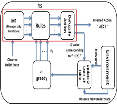
Takagi-Sugeno FISs, since the other type (first-order) calls for a lot more computational cost than zero-order, besides adding more complexity [74]. FIS is presented by a set of rules. 𝑅. with a rule. 𝑗∈𝑅. In the FQL, the. defined as:. IF (𝑏1 𝑖𝑠 𝐿1𝑗 ) . . . AND (𝑏𝑛 𝑖𝑠 𝐿𝑛𝑗 ) . . . AND (𝑏𝑁 𝑖𝑠 𝐿𝑁 𝑗 ) THEN 𝑜𝑗 with 𝑞(𝐿𝑗 , 𝑜𝑗 ).. 𝐿𝑛𝑗 an. is the linguistic label (fuzzy label) of the input variable. 𝑁 -dimensional. rule.. 𝑜𝑗. belief state vector. b = [𝑏1 , . . . , 𝑏𝑛 , . . . , 𝑏𝑁 ]). is an possible output action of the. responding q-value.. 𝑗 th. rule while. 𝑏𝑛 (𝑛th. component of. participating in the. 𝑞(𝐿𝑗 , 𝑜𝑗 ). We build the FIS with competing actions. 𝑜𝑗. 𝑗 th. denotes its cor-. for each rule.. A. schematic diagram for the FQL architecture and its interaction with the environment can be observed in Fig. 2.4. The learning agent has to find the best conclusion for each rule, i.e. the action with the best q-value among the possible discrete actions for each rule. The q-values are zeroed initially and are not significant in the first stages of the learning process. In order to explore the set of possible actions and acquire experience through the reinforcement signals (rewards), the actions for each rule are selected using an exploration exploitation policy (EEP) as [17]. The. 𝜀-greedy method. is used as the EEP policy for choosing the actions:. ⎧ ⎪ ⎨ 𝑜𝑗 = argmax 𝑞(𝐿𝑗 , 𝑜𝑘 ). : 𝑤𝑖𝑡ℎ 𝑝𝑟𝑜𝑏𝑎𝑏𝑖𝑙𝑖𝑡𝑦 1 − 𝜀. 𝑘∈𝐴. ⎪ ⎩ 𝑜𝑗 = random (𝑜𝑘 ) 𝑘∈𝐴. where. 𝜀. (2.5). : 𝑤𝑖𝑡ℎ 𝑝𝑟𝑜𝑏𝑎𝑏𝑖𝑙𝑖𝑡𝑦 𝜀. determines the tradeoff between exploration and exploitation, and. set of all possible actions for each rule or for each component state vector. b.. As stated above, the rule. 𝑗. 𝑏𝑛. 𝐴. is the. of the input belief. is defined by the intersection (with respect. to a T-Norm) of fuzzy sets along each dimension. 𝐿1𝑗 , . . . , 𝐿𝑁 𝑗. 𝜇𝐿1𝑗 (𝑏1 ), . . . , 𝜇𝐿𝑁𝑗 (𝑏𝑁 ). are the membership functions, re-. (where. 𝜇𝐿1𝑗 (𝑏1 ). and. 𝜇𝐿𝑁𝑗 (𝑏𝑁 ). with the truth degrees. spectively defined on the first and the last component of the input belief state vector. b. in rule. 𝑗). and the T-Norm is implemented by product. Hence, the degree of truth. in the fuzzy logic terminology (or the membership of the vector. 36. b). for rule. 𝑗. can be.

written as follows:. 𝛼𝑗 (b) =. 𝑁 ∏︁. 𝜇𝐿𝑛𝑗 (𝑏𝑛 ).. (2.6). 𝑛=1 Furthermore, the following normalization condition should be satisfied:. ∑︁. 𝛼𝑗 (b) = 1.. (2.7). 𝑗∈𝑅. Next, the relation between the inferred action (the output action of the FIS that will be executed at the decision epoch) for an input belief state vector rule actions. 𝑜𝑗 ,. b,. and the applied. is derived as:. 𝑎(b) =. ∑︁. 𝛼𝑗 (b) 𝑜𝑗. (2.8). 𝑗∈𝑅. where the summation is performed over all rules.. For the obtained inferred action. 𝑎(b), a Q-function is also approximated by the FIS output, which is inferred from the quality (q-value) of the local discrete actions that constitute the global continuous action. 𝑎(b).. Under the same assumptions used for generation of. 𝑎(b), the Q-function. is calculated as:. 𝑄(b, 𝑎(b)) =. ∑︁. 𝛼𝑗 (b) 𝑞 (𝐿𝑗 , 𝑜𝑗 ) .. (2.9). 𝑗∈𝑅. We use the value function for the input belief state vector. 𝑉 (b) =. ∑︁. defined here as:. 𝛼𝑗 (b) max 𝑞 (𝐿𝑗 , 𝑜𝑘 ) .. ∆𝑄 is defined as the variation of the quality 𝑄(b, 𝑎(b)),. in other words, the difference between the old and new values of by. (2.10). 𝑘∈𝐴. 𝑗∈𝑅. In order to update the q-values,. b. 𝑄(b, 𝑎(b)).. Denote. 𝑐 the new input belief state vector after taking the action 𝑎(b) for the input belief. state vector. b,. and receiving the reward. 𝑟. from the environment (the natural reward. for RL methods in CR tasks such as spectrum sensing, is related to the CR user’s. 37.

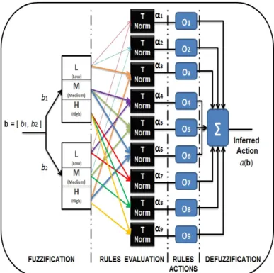
Fig. 2.4. Interaction between the FQL module and the environment (“Environment” is a term that is used to refer to anything outside the sensing device.. Here, the. received reward is related to the CR user’s throughput). throughput. This information may be easily obtained during the online operation of the CR system).. ∆𝑄. is calculated by:. ∆𝑄 = 𝑟 + 𝛾𝑉 (𝑐) − 𝑄(b, 𝑎(b)). Now, the update equation for the q-values is given by (2.12). The symbol. (2.11). 𝑡 is added. to highlight the time dependency in the update equation.. (︀ )︀ (︀ )︀ 𝑞 𝑡+1 (𝐿𝑗 , 𝑜𝑗 ) = 𝑞 𝑡 (𝐿𝑗 , 𝑜𝑗 ) + 𝜅𝛼𝑗 b𝑡 (𝑟𝑡 + 𝛾𝑉 𝑡 b𝑡+1 −𝑄𝑡 (b𝑡 , 𝑎(b𝑡 )) where. 𝜅. is a learning rate. We remind that. the chosen actions. 𝑜𝑗. 𝑞 𝑡 (𝐿𝑗 , 𝑜𝑗 ). (2.12). are the q-values associated to. in all rules. Here, to summarize the FQL-based channel sensing. process, an iterative procedure is prepared as can be observed as Table 2.1. Moreover, to clarify the FIS unit structure as well as its rule over the channel sensing process, see the example drawn in Fig. 2.5 which presents the FIS model for a 2-dimensional belief state vector. b = [𝑏1 , 𝑏2 ]. as the input for the FIS. As mentioned before, the inferred. 38.

Fig. 2.5. Structure of the FIS model with 2-dimensional belief state vector action. 𝑎(b) is the output of the FIS. Obviously, under the same assumptions used for. generation of. 𝑎(b),. the other output for the FIS (i.e. the Q-function:. 𝑄(b, 𝑎(b)). can. be obtained. As shown in Fig. 2.5, for a 2-dimensional belief state vector, 9 fuzzy rules are expected (each color erepresents one rule).. 2.4 Simulation Results 2.4.1 FIS Unit Configurations In this section, we consider a single agent POMDP, including only one MN (and its associated SNs). Therefore, the input belief state vector for the FIS is. b = [𝑏1 ].. As. mentioned, the simulation results can be easily extended to a multi-agent POMDP problem with the input belief state vector. b = [𝑏1 , . . . , 𝑏𝑛 , . . . , 𝑏𝑁 ] which requires some. consideration about the type of cooperation between the MNs. As stated, we focus on a single agent POMDP with. b = [𝑏1 ].. The problem has therefore two states, “0” (the. PU is inactive in the operating channel) and “1” (the PU is active in the operating channel). Thus, state. 𝑏1 = (𝜋 0,𝑡 , 𝜋 1,𝑡 ),. 𝑖 at 𝑡th decision epoch.. where as mentioned before,. Since. 𝜋 1,𝑡 = 1 − 𝜋 0,𝑡 39. 𝜋 𝑖,𝑡. is the probability of. we can use only one probability. 𝜋 1,𝑡.

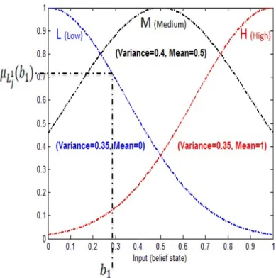
Fig. 2.6. Three fuzzy sets for the belief state. to specify. 𝑏1. and the belief state vector is thus specified by. b = [𝑏1 = 𝜋 1,𝑡 ].. The belief. space for the MN is specified by [0 1] (a continuous space). Here, we partition the belief state. b. into three fuzzy subsets thereby generating three rules (Note that for. a multi-agent POMDP with. b = [𝑏1 , . . . , 𝑏𝑛 , . . . , 𝑏𝑁 ],. we have. 3𝑁. rules). It should be. noted that, more detailed partitions yield exponentially growing state space (rule base size), elongating the adaptation time, and dramatically increasing the computational resource demand, while less detailed partitions (containing only a few member fuzzy sets) could cause less approximation accuracy, or unadaptable situation. Therefore, there is a tradeoff between the computational complexity and approximation accuracy, regarding the number of the fuzzy sets. Linguistic terms for these fuzzy sets are (L, M, H), where L stands for “low”, M is “medium” and H stands for “high”. As depicted in Fig. 2.6, the membership function (fuzzy sets) for the belief state function [27].. b is assumed to be the standard Gaussian membership. The use of various types of membership functions (e.g., linear func-. tions, triangular, trapezoidal and smoother functions such as the symmetric Gaussian function) can affect the performance of the fuzzy logic controller and corresponding. 40.

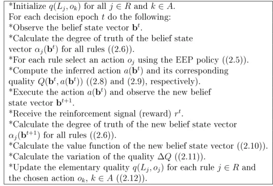
Table 2.1. The iterative procedure adapted for FQL-based channel sensing *Initialize. 𝑞(𝐿𝑗 , 𝑜𝑘 ). for all. For each decision epoch. 𝑗∈𝑅. and. 𝑘 ∈ 𝐴.. 𝑡. do the following: 𝑡 *Observe the belief state vector b . *Calculate the degree of truth of the belief state 𝑡 vector 𝛼𝑗 (b ) for all rules ((2.6)).. 𝑜𝑗 using the EEP policy ((2.5)). 𝑡 *Compute the inferred action 𝑎(b ) and its corresponding 𝑡 𝑡 quality 𝑄(b , 𝑎(b )) ((2.8) and (2.9), respectively). 𝑡 *Execute the action 𝑎(b ) and observe the new belief 𝑡+1 state vector b . 𝑡 *Receive the reinforcement signal (reward) 𝑟 . *For each rule select an action. *Calculate the degree of truth of the new belief state vector 𝛼𝑗 (b𝑡+1 ) for all rules ((2.6)). *Calculate the value function of the new belief state vector ((2.10)).. ∆𝑄 ((2.11)). 𝑞(𝐿𝑗 , 𝑜𝑗 ) for each rule 𝑗 ∈ 𝑅. *Calculate the variation of the quality *Update the elementary quality the chosen action. 𝑜𝑘 , 𝑘 ∈ 𝐴. and. ((2.12)).. change in the system output (FQL output, i.e., the inferred action learned by the MN) when we change the type of the membership function on the same system. However, the selection of membership function type is out of the scope of this thesis. As mentioned, in this thesis, we use Gaussian function which is more preferable as it provides better smoothness and easy to describe the generation of new fuzzy rules [27].. It should be noted that the inferred action. 𝑎(b). applied to the environment by the MN. However, since. as the output of the FIS is. 𝑎(b). is a continuous action,. its value may not be an integer while this value specifying the action’s type (Data Transmission, Stop Data Transmission or Channel Switching) for the MN, should be an integer. Thus, we use the round off principle to quantize the value of. 𝑎(b). to an. integer. A “collision” occurs between the PU and the CR network when the CR nodes (as the SNs related to the MN in the presented model) transmit data while the operating channel is occupied by the PU. Reinforcement signal (reward). 𝑟. penalizes the. CR network whenever a collision occurs between the CR network and the PU. In this case, the CR network is penalized by a negative fixed value, i.e.. −5.. Accordingly, if. the CR network performs channel switching whether the PU is active or inactive over the operating channel, the penalty value is. 41. −0.5.. Note that if less-frequent channel.

switching is preferred for stability, a more negative value can be chosen. The reward. 𝑟. should be a positive value when user data are successfully transmitted by the SNs. without collision, i.e.. +5.. On the other hand, If stop data transmission (regardless. the PU state) is chosen, then the time is consumed without transmitting any data, and therefore. 𝑟. should be zero. The values of the rewards can be varied to control. the tradeoff between the channel utilization and the collision probability. For example, we can reduce the collision probability at the expense of channel utilization by decreasing the value of. 𝑟. from. +5. to. +2. [27].. 2.4.2 Numerical Evaluations To show the performance of the FQL algorithm and its supremacy against the QL algorithm, different figures were depicted. The main goal is that the CR network has to avoid any collision with the PU and at the same time achieving the maximum channel utilization. Indeed, the “channel utilization” is defined as the proportion of time in which the CR networks successfully exchange data without collision with the PU. In other words, the final purpose is to maximize the total discounted reward. This value is a figure of merit for the quality of the learned policy, i.e., how much reward the CR accumulates while following the optimal policy. The parameter values used in this chapter are. 𝜅 = 0.8, 𝛾 = 0.995, 𝜀 = 0.3, 𝜂 = 0.5, 𝑇𝑐 = 1. ms,. 𝑇 = 0.1. ms. and the SNR of the PU signal is -10 dB (the optimal values of the FQL parameters can be obtained with the help of a genetic algorithm without any prior information as in [75]). The transition probability. ⎛ ⎝. 𝑃0,0 𝑃0,1 𝑃1,0 𝑃1,1. ⎞. ⎛. ⎠=⎝. 𝑃𝑖,𝑗. is also governed by the following matrix:. 0.98 0.02 0.02 0.98. ⎞ ⎠.. (2.13). Furthermore, in the EEP strategy, we gradually reduce the value of exploration parameter. 𝜀. after each decision epoch using the following equation:. 𝜀 = 𝜀 × 0.995.. (2.14). 42.

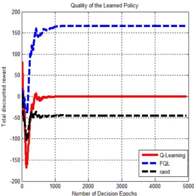
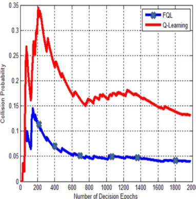
Fig.. 2.7 shows the reward accumulation results for the FQL and QL algorithms. as well as a random selection method (where the action regarding the MN’s belief state at each decision epoch is selected randomly). As shown in this figure, the FQL achieves the highest sum of discounted reward. Clearly, use of the FIS decision unit allows the agent to quickly and efficiently achieve the optimal policy. Thus, using the FQL, the CR network can accumulate more reward while following the optimal policy. Realization of such high performance is an indicator of the quality of learned policy. Fig. 2.8 illustrates the collision probability between the PU and the CR network. The “collision probability” is defined as the proportion of time in which the CR network transmits data when the operating channel is in use by the PU. Results show that the collision probability when the FQL algorithm is used for discovering the optimal policy is always lower than that when the QL is used. As it is seen in this figure, at the beginning of the learning process (at the initial decision epochs), whenever the PU is in active state or appears in the operating channel, the collision probability is high, and this is because of the wrong decisions made by the CR network from lack of experience regarding the PU state. However, as time goes on and the optimal policy is discovered by the MN (using the RL algorithms), the collision probability is low even in those times that the PU is active or appears in the operating channel. Fig. 2.9 (a), (b) and (c) respectively shows the PU activity on the operating channel (of course, the MN is unaware of the PU activity, but can learn it using the RL), the instantaneous reward gained by the CR network equipped with the QL and the instantaneous reward gained by the CR network equipped with the FQL. Indeed, the instantaneous reward gives more information about the higher performance of the FQL. The FQL based scheme for the CR network got more rewards and fewer penalties, since use of FIS allows the CR network to quickly and stably zero-in on the optimal policy. As a result, higher channel utilization and lower collision probability are achieved.. 43.

Fig. 2.7. Total discounted reward of different strategies. 2.5 Estimation of the State Transition Probabilities To obtain the simulation results in Figs. 2.7, 2.8 and 2.9, we assumed that the state transition probabilities (𝑃𝑖,𝑗 ) of the PU (in the belief state formula) are known to the CR as in different studies (e.g., [62], and [63]), which is in most cases not true in the real world. Hence, even though the concept of sensing is valid literally, its practical application is severely limited [76], [77]. Thus quite realistically, the channel state transition probabilities are assumed to be unknown. On the other hand, during the whole operation time, the channel state transition probabilities are assumed to be constant; and these values are estimated by the CR network.. These transition. probabilities can be estimated using the Baum-Welch Algorithm (BWA) [78], which is basically a derived form of the Expectation Maximization (EM) algorithm for hidden Markov models (HMMs) [78].. The concept of an HMM extends directly from. Markov models, with the observation being a probabilistic function of the state. An HMM is a doubly embedded stochastic process with an underlying process that is not observable (the hidden state), but can only be observed through another set of stochastic process that produces the sequence of observations [78]. Though a Markov. 44.

Fig. 2.8. The collision probability comparison: FQL vs. QL.. chain is appropriate in modeling the PU’s channel access pattern, the true states of the PU are never known to the CR at any particular sampling instant.. What the. CR network can observe directly is some signal “emitted” from a particular state (The received PU signal). The received signal fits into a hidden Markov model [79]. The Baum-Welch algorithm can be employed to process input observation sequences (received at the MN) and generate parameters of HMMs. Training is usually done offline. The parameters of the HMM are obtained after the training phase and stored for future use. In other words, the state transition probabilities of the PU (as one of the HMM’s parameters) are estimated first, and then it will be used in the POMDP framework, as previously described.. The general approach is to train the model. with the observation data using some iterative procedure until its convergence. More specifically, the parameter set. 𝜆 = (𝐴, 𝐵, 𝜋). guesses at first; a set of transition probabilities. would be initialized with appropriate. 𝐴 = {𝑝𝑖,𝑗 }, 𝑖, 𝑗 ∈ {0, 1}, 𝐵 = 𝑏𝑖 (𝑌𝑡 ). is. the observation symbol probability (also called emission probability) distribution in state. 𝑖 (𝑖 ∈ {0, 1}). (we will use. 𝑌𝑡. which can be easily obtained from the pmf ’s of the sensing results. to denote the observation symbol at time 𝑡), and finally. 45. 𝜋. is the initial.

(a). (b). (c). Fig. 2.9. (a) The PU activity on the operating channel. (b) Instantaneous reward for the QL based CR network. (c) Instantaneous reward for the FQL based CR network.. state probabilities. 𝜋 = {𝜋 𝑖 }, 𝑖 ∈ {0, 1}.. Then a set of re-estimation formula would be. repeatedly used in a number of iterations so that the parameter set could gradually approach to the ideal values where the occurrence possibility of the observation sequence is maximized. Let time. 𝑡. 𝜉𝑡 (𝑖, 𝑗). be the probability of the HMM being in state. and making a transition to state. of the model. 𝜆 = (𝐴, 𝐵, 𝜋). 𝑗. at time. 𝑡+1,. and observation sequence. 𝑖. at. given the appropriate guesses. Y = {𝑌1 , 𝑌2 , ... , 𝑌𝑇 }. as the. partial observation sequence received at the CR network (The signal received at time. 𝑡. (observation symbol,. i.e.,. 𝑌𝑡 = 𝑠𝑡 𝑋𝑡 + 𝑈𝑡. 𝑌𝑡 ). where. at the CR, is a noisy version of the PU’s actual signal,. 𝑋𝑡. is the PU’s signal, and. 𝑈𝑡. Gaussian noise (AWGN) with mean zero and variance. 𝜉𝑡 (𝑖, 𝑗) = 𝑃 (𝑠𝑡 = 𝑖, 𝑠𝑡+1 = 𝑗|Y, 𝜆) .. is modeled as additive white. 𝜎 2 ): (2.15). With the first-order Markov assumption, the received samples in the observation sequence are conditionally independent given the state sequence. In other words, the probability distribution of generating current observation symbol depends only on the current channel state, i.e.,. 𝑃 (Y|s, 𝜆) =. ∏︁ 𝑇 𝑡=1 46. 𝑃 (𝑌𝑡 |𝑠𝑡 , 𝜆). (2.16).

where. s = {𝑠1 , 𝑠2 , ... , 𝑠𝑇 }. denotes the hidden channel state sequence. Using Bayes. law and the independency assumption, (2.15) follows:. 𝛼𝑡 (𝑖) 𝑝𝑖,𝑗 𝑏𝑗 (𝑌𝑡+1 ) 𝛽 𝑡+1 (𝑗) 𝑃 (Y|𝜆). (2.17). (︀ )︀ 𝛼𝑡 (𝑖) = 𝑃 𝑠𝑡 = 𝑖, Y(𝑡) |𝜆 , 𝛽 𝑡 (𝑖) = 𝑃 (Y*(𝑡) |𝑠𝑡 = 𝑖, 𝜆) and 𝑃 (Y|𝜆) are forward probabilities, backward probabilities and observation probability (the pmf ’s of the observation sequence. Y given the parameter set 𝜆), respectively, where Y(𝑡) = {𝑌1 , ... , 𝑌𝑡 } is. the partial observation sequence up to time time series beyond time up to time. 𝑡. 𝑡.. 𝛼𝑡 (𝑖). Therefore,. 𝑖. and in state. at time. 𝑡 and Y*(𝑡) = {𝑌𝑡+1 , ... , 𝑌𝑇 }, the partial is the probability of partial observations. 𝑡. 𝛼𝑡 (𝑖). is proportional to the likelihood of the. past observations and can be solved recursively according to:. 𝛼1 (𝑖) = 𝑃 (𝑌1 ; 𝑠𝑡 = 𝑖) = 𝜋 𝑖 𝑏𝑖 (𝑌1 ). 𝛼𝑡 (𝑖) =. ∑︁. (2.18). [𝛼𝑡−1 (𝑗) 𝑝𝑗,𝑖 ]𝑏𝑖 (𝑌𝑡 ). (2.19). 𝑗∈{0,1}. for. 2 ≤ 𝑡 ≤ 𝑇.. In a very similar manner,. observation sequence from at the. 𝑖th. 𝑌𝑡+1. state. By definition,. 𝛽 𝑡 (𝑖). is the probability of the partial. to the end produced by all state sequences that start. 𝛽 𝑇 (𝑖) = 1. 𝛽 𝑡 (𝑖). is proportional to the likelihood of. the future observations and can be solved recursively according to:. 𝛽 𝑡 (𝑖) =. ∑︁. 𝛽 𝑡+1 (𝑗) 𝑝𝑖,𝑗 𝑏𝑗 (𝑌𝑡+1 ). (2.20). 𝑗∈{0,1}. for. 𝑡 = 𝑇 − 1, 𝑇 − 2, ..., 1.. Finally, the normalization factor. 𝑃 (Y|𝜆) can be calculated. in the following ways:. 𝑃 (Y|𝜆) =. ∑︁ 𝑖∈{0,1}. 47. 𝛼𝑇 (𝑖). (2.21).

∑︁. 𝑃 (Y|𝜆) =. 𝜋 𝑖 𝑏𝑖 (𝑌1 ) 𝛽 1 (𝑖). (2.22). 𝑖∈{0,1}. 𝑃 (Y|𝜆) =. ∑︁. 𝛼𝑡 (𝑖) 𝛽 𝑡 (𝑖). (2.23). 𝑖∈{0,1}. for any. 1 ≤ 𝑡 ≤ 𝑇.. Thus the desired probability is simply computed by summing all. the forward and backward products as in (2.23). The recursive computation structure of the forward probabilities is illustrated in the trellis of Fig. 2.10. We also define. 𝛾 𝑡 (𝑖) as the probability of being in state 𝑖 at time 𝑡 given the observation sequence Y and the model. 𝜆,. then it can be proven:. 𝛾 𝑡 (𝑖) = 𝑃 (𝑠𝑡 = 𝑖|Y, 𝜆). 𝛾 𝑡 (𝑖) =. 𝑃 (𝑠𝑡 = 𝑖, Y|𝜆) 𝑃 (Y|𝜆). (︀ )︀ 𝑃 𝑠𝑡 = 𝑖, Y(𝑡) |𝜆 𝑃 (Y*(𝑡) |𝑠𝑡 = 𝑖, 𝜆) 𝛾 𝑡 (𝑖) = 𝑃 (Y|𝜆). 𝛾 𝑡 (𝑖) =. 𝛼𝑡 (𝑖) 𝛽 𝑡 (𝑖) . 𝑃 (Y|𝜆). (2.24). Note that. 𝑇 −1 ∑︁. 𝛾 𝑡 (𝑖) = 𝑒𝑥𝑝𝑒𝑐𝑡𝑒𝑑 𝑁 𝑜. 𝑜𝑓 𝑡𝑟𝑎𝑛𝑠𝑖𝑡𝑖𝑜𝑛𝑠 𝑓 𝑟𝑜𝑚 𝑠𝑡𝑎𝑡𝑒 𝑖.. (2.25). 𝜉𝑡 (𝑖, 𝑗) = 𝑒𝑥𝑝𝑒𝑐𝑡𝑒𝑑 𝑁 𝑜. 𝑜𝑓 𝑡𝑟𝑎𝑛𝑠𝑖𝑡𝑖𝑜𝑛𝑠 𝑓 𝑟𝑜𝑚 𝑠𝑡𝑎𝑡𝑒 𝑖 𝑡𝑜 𝑠𝑡𝑎𝑡𝑒 𝑗.. (2.26). 𝑡=1. 𝑇 −1 ∑︁ 𝑡=1. 48.

𝛾 𝑡 (𝑖). is shown to be related to. 𝜉𝑡 (𝑖, 𝑗). 𝛾 𝑡 (𝑖) =. by. 2 ∑︁. 𝜉𝑡 (𝑖, 𝑗) .. (2.27). 𝑗=1. With the above definitions, we can outline the Baum-Welch re-estimation formula:. 𝜋 ˆ 𝑖 = 𝑒𝑥𝑝𝑒𝑐𝑡𝑒𝑑 𝑓 𝑟𝑒𝑞𝑢𝑒𝑛𝑐𝑦 𝑖𝑛 𝑠𝑡𝑎𝑡𝑒 𝑖 𝑎𝑡 𝑡𝑖𝑚𝑒 𝑡 = 1 = 𝛾 1 (𝑖). (2.28). 𝑒𝑥𝑝𝑒𝑐𝑡𝑒𝑑 𝑁 𝑜. 𝑜𝑓 𝑡𝑟𝑎𝑛𝑠𝑖𝑡𝑖𝑜𝑛𝑠 𝑓 𝑟𝑜𝑚 𝑠𝑡𝑎𝑡𝑒 𝑖 𝑡𝑜 𝑗 𝑃𝑖,𝑗 = 𝑒𝑥𝑝𝑒𝑐𝑡𝑒𝑑 𝑁 𝑜. 𝑜𝑓 𝑡𝑟𝑎𝑛𝑠𝑖𝑡𝑖𝑜𝑛𝑠 𝑓 𝑟𝑜𝑚 𝑠𝑡𝑎𝑡𝑒 𝑖 ∑︀𝑇 −1 ∑︀𝑇 −1 𝛼𝑡 (𝑖) 𝑝𝑖,𝑗 𝑏𝑗 (𝑌𝑡+1 ) 𝛽𝑡+1 (𝑗) 𝑡=1 𝜉𝑡 (𝑖, 𝑗) = ∑︀𝑇 −1 = 𝑡=1 ∑︀𝑇 −1 𝑡=1 𝛾 𝑡 (𝑖) 𝑡=1 𝛼𝑡 (𝑖) 𝛽 𝑡 (𝑖). (2.29). ˆ𝑏𝑖 (𝑚)= 𝑒𝑥𝑝𝑒𝑐𝑡𝑒𝑑 𝑁 𝑜. 𝑜𝑓 𝑡𝑖𝑚𝑒𝑠 𝑖𝑛 𝑠𝑡𝑎𝑡𝑒 𝑖 𝑎𝑛𝑑 𝑜𝑏𝑠𝑒𝑟𝑣𝑖𝑛𝑔 𝑈𝑚 𝑒𝑥𝑝𝑒𝑐𝑡𝑒𝑑 𝑁 𝑜. 𝑜𝑓 𝑡𝑖𝑚𝑒𝑠 𝑖𝑛 𝑠𝑡𝑎𝑡𝑒 𝑖. ∑︀𝑇 =. where. 𝑡=1, 𝑌𝑡 =𝑈𝑚 𝛾 𝑡 ∑︀𝑇 𝑡=1 𝛾 𝑡 (𝑖). (𝑖). (2.30). 𝑈𝑚 is the 𝑚th symbol in the observation alphabet (here we have two observation. symbols (active and inactive) in alphabet size representing the PU state). Suppose we have an initial guess of the parameters of the HMM. 𝜆0 = (𝐴0 , 𝐵0 , 𝜋 0 ). and several. sequences of observations, then using (2.25) and (2.26), we can calculate the expected values of transition properties of the Markov Chain (the Expectation step of EM algorithm). Then the maximum likelihood estimation of the model is computed through the recursive usage of (2.28)-(2.30) (the Maximization step of EM algorithm). It can be proven [80] that after each iteration and gaining a new parameters of the HMM, the received observation sequences can be better explained by the new model. The. 𝜆. is iteratively re-estimated until it converges to a limit point. It should be remembered that the Baum-Welch method leads to a local maximum of. 49. 𝜆 only.. In practice, to get.

a good solution, the initial guess guesses of. 𝜆0. 𝜆0. is very important. Usually several sets of starting. are used and one with the greatest likelihood value is chosen.. Laird. suggested a grid search method [80] which divides the searching domain into small grids and starts from each of the intersections. Leroux and Puterman argue that the grid method would generate too many initial points when high dimensional spaces are involved. They suggest a clustering algorithm and a simple implementation can be found in [81]. The independence assumption we made was between the symbols of the single observation sequence. Y = {𝑌1 , 𝑌2 , ... , 𝑌𝑇 }.. window to collect symbols in an observation sequence.. We consider a short time. Symbols collected within a. short time window on the PU activity have negligible correlation as shown in [81]. Therefore, the independence assumption made between the symbols in an observation sequence is to facilitate the mathematical computations and it is a reasonable assumption. However, the major problem with the estimation method is that only a single observation sequence (from a short time window) to train the model is not enough [78]. Hence, in order to have sufficient data to make acceptable estimates of the parameter set. 𝜆,. we have to use multiple observation sequences. On the other. hand, the most important issue is that for a set of observation sequences in a real and practical system, one cannot say these observation sequences are independent from each other [83].. Generally speaking, in real scenarios, these observation sequences. are statistically correlated. A controversy can arise if one assumes the independence property while these observation sequences are statistically correlated.. Now let us. consider a set of observation sequences from a pattern class:. O = {Y(1 ) , Y(2 ) , ... , Y(L) }. (2.31). where. (𝑙). (𝑙). (𝑙). Y(𝑙) = {𝑌1 , 𝑌2 , ... , 𝑌𝑇 }, 1 ≤ 𝑙 ≤ 𝐿. 50. (2.32).

Without loss of generality we have the following expressions. ⎧ ⎪ ⎪ 𝑃 (O|𝜆) = 𝑃 ⎪ ⎪ ⎪ ⎪ ⎨ 𝑃 (O|𝜆) = 𝑃 ⎪ ⎪ ... ⎪ ⎪ ⎪ ⎪ ⎩ 𝑃 (O|𝜆) = 𝑃. (︀ (1) )︀ Y |𝜆 𝑃 (︀ (2) )︀ Y |𝜆 𝑃. (︀ (2) (1) )︀ Y |Y , 𝜆 ... 𝑃 (︀ (3) (2) )︀ Y |Y , 𝜆 ... 𝑃. (︀. )︀ Y(𝐿) |Y(𝐿−1) ... Y(1) , 𝜆 (︀ (1) (𝐿) )︀ Y |Y ... Y(2) , 𝜆. (︀ (𝐿) )︀ (︀ (1) (𝐿) )︀ (︀ )︀ Y |𝜆 𝑃 Y |Y , 𝜆 ... 𝑃 Y(𝐿−1) |Y(𝐿) Y(𝐿−2) ... Y(1) , 𝜆 (2.33). Based on the above expressions, it is easy to see that the multiple observation sequence probability can be expressed as a combination of individual observation probabilities, i.e.,. 𝑃 (O|𝜆) =. 𝐿 ∑︁. (︀ )︀ 𝑤𝑙 𝑃 Y(𝑙) |𝜆. (2.34). 𝑙=1 in which,. ⎧ (︀ (2) (1) )︀ (︀ (𝐿) (𝐿−1) )︀ 1 (1) ⎪ ⎪ 𝑤 = 𝑃 Y |Y , 𝜆 ... 𝑃 Y |Y ... Y , 𝜆 1 ⎪ 𝐿 ⎪ ⎪ ⎪ ⎨ 𝑤 = 1 𝑃 (︀Y(3) |Y(2) , 𝜆)︀ ... 𝑃 (︀Y(1) |Y(𝐿) ... Y(2) , 𝜆)︀ 2 𝐿 ⎪ ⎪ ... ⎪ ⎪ ⎪ ⎪ ⎩ 𝑤 = 1 𝑃 (︀Y(1) |Y(𝐿) , 𝜆)︀ ... 𝑃 (︀Y(𝐿−1) |Y(𝐿) Y(𝐿−2) ... Y(1) , 𝜆)︀ 𝐿 𝐿 (2.35). are weights.. These weights are conditional probabilities and hence they can char-. acterize the dependence-independence property. Based on the above equations, the modification of corresponding re-estimation equations in (2.28), (2.29) and (2.30) are respectively as follows [83]. ∑︀𝐿 𝜋 ˆ𝑖 =. 𝑙=1. (︀ )︀ 𝑤𝑙 𝑃 Y(𝑙) |𝜆 𝛾 𝑙1 (𝑖). ∑︀𝐿. 𝑙=1. 𝑤𝑙 𝑃 (Y(𝑙) |𝜆). 51. (2.36).

Table 2.2. Transition probabilities estimation as a function of the data set for training model (at SNR = −2 dB). )︂ 𝑃𝑖,𝑗. Original Parameter. (︂. 0.98 0.02 0.02 0.98. Test set 1(300 data). (︂. 0.7114 0.2886 0.3415 0.6585. )︂. Test set 2(1000 data). (︂. 0.8000 0.2000 0.2544 0.7456. (a). 𝑡,. and states. 𝑖.. Test set 3(5000 data). (︂. 0.9300 0.0700 0.0821 0.9179. (b). Fig. 2.10. (a) Implementation of Computation of vations. )︂. 𝛼𝑡 (𝑖). in terms of a lattice of obser-. (b) Computing the forward probabilities.. (︁ )︁ ∑︀𝑇𝑙 −1 𝑙 (𝑙) 𝑙 (𝑙) |𝜆 𝑤 𝑃 Y 𝛼 (𝑖)𝑝 𝑏 𝑌 ( ) 𝑖,𝑗 𝑗 𝑡 𝑙=1 𝑙 𝑡=1 𝑡+1 𝛽 𝑡+1 (𝑗) ∑︀𝐿 ∑︀𝑇𝑙 −1 𝑙 𝑙 (𝑙) 𝑙=1 𝑤𝑙 𝑃 (Y |𝜆) 𝑡=1 𝛼𝑡 (𝑖)𝛽 𝑡 (𝑖). ∑︀𝐿. 𝑃𝑖,𝑗 =. (︀ )︀ ∑︀𝑇𝑙 𝑙 𝑙 𝑤𝑙 𝑃 Y(𝑙) |𝜆 𝑡=1, 𝑌𝑡 =𝑈𝑚 𝛼𝑡 (𝑖)𝛽 𝑡 (𝑖) ∑︀𝑇𝑙 𝑙 ∑︀𝐿 𝑙 (𝑙) 𝑡=1 𝛼𝑡 (𝑖)𝛽 𝑡 (𝑖) 𝑙=1 𝑤𝑙 𝑃 (Y |𝜆). (2.37). ∑︀𝐿 ˆ𝑏𝑖 (𝑚) =. 𝑙=1. (2.38). However, in [78] the author assumes that each observation sequence is independent from every other sequence, i.e.,. 𝑃 (O|𝜆) =. 𝐿 ∏︁. (︀ )︀ 𝑃 Y(𝑙) |𝜆. (2.39). 𝑙=1. Figs. 2.11, 2.12, 2.13 and 2.14 illustrate the following: without any a priori information about the channel characteristics, even in a very transient environment, it is quite possible to achieve reasonable estimates of channel state transition probabilities with a practical and simple implementation. They show the estimates of the channel. 52. )︂.

transition probabilities as a function of the SNR parameter for the observation set with a length of 1000. It is important to note that the estimates improve by increasing the SNR values, hence allowing better performance for the proposed sensing method in the previous sections. We initialized. ⎛ 𝜆0 = (⎝. 0.85 0.15 0.1. 0.9. ⎞ ⎛ ⎠,⎝. 1 0 0 1. 𝜆0 = (𝐴0 , 𝐵0 , 𝜋 0 ). as follows:. ⎞ ⎠ , (𝜋 0 = 0.2. 𝜋 1 = 0.8)). Clearly, the estimates also improve as the data set for the training model increases (see Table 2.2). As seen in Table 2.2, the parameter of SNR is not the only factor affecting the accuracy of estimation. Table 2.2 shows the accuracy of the estimates according to the length of the data set. We can see that the estimates become more and more accurate as the data set for the training model increases. In this example, we can get sufficiently accurate estimates from 5,000 training data even at a low SNR value of -2dB.. Fig. 2.11. Transition probabilities. 53. 𝑃0,0. estimation.

Fig. 2.12. Transition probabilities. 𝑃0,1. estimation. Fig. 2.13. Transition probabilities. 𝑃1,0. estimation. 54.

Fig. 2.14. Transition probabilities. 𝑃1,1. estimation. 2.6 Conclusion In this chapter, we have proposed a learning based scheme for channel sensing in partially-sensed CR network.. We introduced a novel fuzzy RL control scheme. in the POMDP framework to successfully address time and complexity issues.. In. particular, the CR network’s channel sensing scheme is formulated as a POMDP, and the optimal policy is determined by a powerful approach such as the FQL algorithm. Using our proposed sensing scheme, the CR network can significantly improve its own spectral efficiency and reduce the probability of interfering with the PU. Simulation results show that high spectrum utilization and very low sensing error probability are achieved via the maximization of the total discounted reward. We have also shown that without any a priori information about the channel characteristics, even in a very transient environment, it is quite possible to achieve reasonable estimates of channel state transition probabilities.. 55.









Φ𝑀. Φ𝐹. λ𝑀. λ𝐹 Φ𝑀. λ𝑀 Φ𝐹. λ𝐹. λ λ = λ𝐹 + λ𝑀 λ𝑀. λ𝐹. 𝑁 𝑀 𝑀≤𝑁.

𝑇 𝑇𝑆 𝑇𝐷 𝑇𝑆𝑅𝐵. 𝑇𝑆. 𝑁𝑠 𝑁 𝑁𝑠. 𝑇𝑆. 𝑇𝐷. 𝑇𝑆 = 𝑇𝑆𝑅𝐵 𝑁𝑠.

𝑃𝑑. 𝑃𝑓 𝑃𝑑 = 1. 𝑃𝑓 = 0. 𝑃𝑑 ≠ 1. 𝑃𝑓 ≠ 0. 𝐷.

𝑝𝑂𝐹 𝜃 𝜃. 𝑝𝑂𝐹 = 1 − 𝑃[SINR > 𝜃]. SINR =. (3.1). 𝑃𝐹 ℎ𝐹 𝑟𝐹 −𝛼 𝜎 2 + 𝐼𝐹𝐵 + 𝐼𝑀𝐵. (3.2). 𝑃𝐹 𝑟𝐹 𝛼.

𝐼𝐹𝐵. 𝐼𝑀𝐵 𝜎2 𝑃𝐹. ℎ𝐹 ~ exp(𝜇). 1/𝜇. 𝑃𝐹 ℎ𝐹 𝑟𝐹 −𝛼 𝑃[SINR > 𝜃] = 𝑃 [ 2 > 𝜃] 𝜎 + 𝐼𝐹𝐵 + 𝐼𝑀𝐵 =̈ 𝑃 [ℎ𝐹 > (𝜎 2 + 𝐼𝐹𝐵 + 𝐼𝑀𝐵 ). 𝜃𝑟𝐹 𝛼 ] 𝑃𝐹. ∞. = ⃛ E𝐼𝐹𝐵 ,𝐼𝑀𝐵 [∫. 𝜃𝑟𝐹 𝛼 𝑃𝐹. [𝜇 exp(−𝜇𝑥)] d𝑥]. (𝜎2 +𝐼𝐹𝐵 +𝐼𝑀𝐵 ) 2. = E𝐼𝐹𝐵 ,𝐼𝑀𝐵 [exp [−𝜇(𝜎 + 𝐼𝐹𝐵 + 𝐼𝑀𝐵 ). ∙∙. 𝜃𝑟𝐹 𝛼 ]] 𝑃𝐹. ∙∙∙. ℎ𝐹. E𝐼𝐹𝐵 ,𝐼𝑀𝐵 [∙] 𝐼𝐹𝐵. 𝑃[SINR > 𝜃] = 𝑒. −𝜇. =𝑒. ℒ𝐼𝐹𝐵 (𝑠) 𝐼𝑀𝐵. (3.3). 𝜃𝑟𝐹 𝛼 2 𝜎 𝑃𝐹. −𝜇. 𝜃𝑟𝐹 𝛼 2 𝜎 𝑃𝐹. . E𝐼𝐹𝐵 [𝑒. −𝜇. 𝜃𝑟𝐹 𝛼 𝐼 𝑃𝐹 𝐹𝐵. ] . E𝐼𝑀𝐵 [𝑒. 𝜃𝑟𝐹 𝛼 𝐼 𝑃𝐹 𝑀𝐵. 𝜃𝑟𝐹 𝛼 𝜃𝑟𝐹 𝛼 . ℒ 𝐼𝐹𝐵 (𝜇 ) . ℒ 𝐼𝑀𝐵 (𝜇 ) 𝑃𝐹 𝑃𝐹. ℒ𝐼𝑀𝐵 (𝑠) 𝑠 𝑠=𝜇. −𝜇. 𝐼𝑀𝐵. ] (3.4). 𝐼𝐹𝐵 𝜃𝑟𝐹. 𝛼. 𝑃𝐹. 𝑝𝑂𝐹 = 1 − E𝑟𝐹 [𝑃[SINR > 𝜃]].

∞. 𝑝𝑂𝐹 = 1 − ∫ [𝑃[SINR > 𝜃]]. 𝑓𝑟𝐹 (𝑟𝐹 ) d𝑟𝐹. (3.5). 0. 2. 𝑓𝑟𝐹 (𝑟𝐹 ) = 𝑒 −λ𝐹𝜋𝑟𝐹 2𝜋λ𝐹 𝑟𝐹. 𝑟𝐹. 𝑟𝐹 ∞. 𝑝𝑂𝐹 = 1 − ∫ 𝑒. −𝜋λ𝐹 𝑟𝐹 2. .𝑒. −𝜇. 𝜃𝑟𝐹 𝛼 2 𝜎 𝑃𝐹. 0. 𝑃𝑑 = 1. 𝜃𝑟𝐹 𝛼 𝜃𝑟𝐹 𝛼 . ℒ 𝐼𝐹𝐵 (𝜇 ) . ℒ𝐼𝑀𝐵 (𝜇 ) . 2𝜋𝑟𝐹 λ𝐹 d𝑟𝐹 (3.6) 𝑃𝐹 𝑃𝐹. 𝑃𝑓 = 0 :. 𝑝𝑅𝐵. E𝐼𝑀𝐵 [𝑒. ∞. 𝑝𝑂𝐹 = 1 − ∫ 𝑒 0. −𝜋λ𝐹 𝑟𝐹 2. .𝑒. −𝜇. 𝜃𝑟𝐹 𝛼 2 𝜎 𝑃𝐹. −𝜇. 𝜃𝑟𝐹 𝛼 𝐼 𝑃𝐹 𝑀𝐵. ]=1. ℒ 𝐼𝑀𝐵 (𝜇. 𝜃𝑟𝐹 𝛼 . ℒ 𝐼𝐹𝐵 (𝜇 ) . 2𝜋𝑟𝐹 λ𝐹 d𝑟𝐹 . 𝑃𝐹. 𝜃𝑟𝐹 𝛼 𝑃𝐹. )=1. (3.7).

𝑓𝑏𝑠0 𝐷 𝜆′𝐹 ≤ λ𝐹 ℒ 𝐼𝐹𝐵 (𝑠) = E𝐼𝐹𝐵 [exp(−𝑠𝐼𝐹𝐵 )] = EΦ𝐹,𝑔𝑖 [exp(−𝑠 ∑𝑖∈Φ𝐹 \{𝑓𝑏𝑠0} 𝑃𝐹 𝑔𝑖 𝑅𝑖−𝛼 )] = EΦ𝐹 [∏. 𝑅𝑖. 𝑖∈Φ𝐹 \{𝑓𝑏𝑠0 }. E𝑔𝑖 [exp(−𝑠𝑃𝐹 𝑔𝑖 𝑅𝑖−𝛼 )]]. (3.8). 𝑖 Φ𝐹. 𝑔𝑖 𝑃𝐹 𝑓(𝑥). E[∏𝑥∈Φ 𝑓(𝑥)] = exp(− ∫ℝ𝑑(1 − 𝑓(𝑥))λ d𝑥 ) ∞. ℒ𝐼𝐹𝐵 (𝑠) = exp {−E𝑔 [∫𝑟 (1 − exp(−𝑠𝑃𝐹 𝑔𝑅 −𝛼 ))𝜆𝐼 (𝑅)d𝑅 ]} 𝐹. (3.9). 𝑟𝐹 𝑟𝐹. ∞ ℝ𝑑 \𝑏(0, 𝑟𝐹 ). y. 𝑏(𝑥, 𝑦). 𝑥. Φ𝐹 𝜆𝐼 (𝑅) = 𝜆′𝐹 𝑑𝑅 𝑑−1 𝑏𝑑. (3.10).

𝑅 ℝ𝑑. 𝑏𝑑. 𝑏𝑑 =. √𝜋 𝑑 , Г(𝑥) Г(1+𝑑⁄2). =. ∞. ∫0 𝑡 𝑥−1 𝑒 −𝑡 d𝑡. 𝑝𝑅𝐵 𝑝𝑅𝐵. 𝑝𝑡𝑥 1 − 𝑝𝑡𝑥. Φ𝐹. Φ𝐹. Φ𝐹. Φ𝐹. 𝑝𝑅𝐵. Φ𝐹. 𝑝𝑅𝐵. 𝜆𝐼 (𝑅) = 𝜆′𝐹 𝑑𝑅 𝑑−1 𝑏𝑑 𝑝𝑅𝐵 𝑝𝑡𝑥. ∞. exp {−𝐸𝑔 [∫ (1 − exp(−𝑠𝑃𝐹 𝑔𝑅 −𝛼 ))𝜆′𝐹 𝑏𝑑 𝑝𝑅𝐵 𝑝𝑡𝑥 𝑑𝑅 𝑑−1 𝑑𝑅 ]} . 𝑟𝐹. (3.11).

𝛼. 𝑅𝑑 → 𝑥. ℒ 𝐼𝐹𝐵 (𝑠) = 𝑒 𝑟𝐹. 𝑑𝑏. 𝑥𝑑 → 𝑦. 𝑑 ′ 𝑑 ′ 𝑑 𝑑 𝑝𝑅𝐵 𝑝𝑡𝑥 𝜆𝐹 −𝛼𝑏𝑑 𝑝𝑅𝐵 𝑝𝑡𝑥 𝜆𝐹 (𝜇𝜃)𝛼 𝑟𝐹 𝑀(𝜃,𝛼). 𝑑. 𝑑. (3.12). 𝑑. (3.13). 𝑀(𝜃, 𝛼) = E [(𝑔)𝛼 (Г (− 𝛼 , 𝜇𝜃𝑔) − Г (− 𝛼))] ∞. Г(𝑎, 𝑥) = ∫𝑥 𝑡 𝑎−1 𝑒 −𝑡 d𝑡 𝑟𝐹 2. 𝑑=2. ∞. 𝑝𝑂𝐹 = 1 − ∫ 𝑒. 𝜋𝑧(𝜆′𝐹 𝑝𝑅𝐵 𝑝𝑡𝑥 −λ𝐹 )−. 𝑧. 2 𝛼 𝜇𝜃 2 2 𝜎 𝑧 2 − 𝜋𝑝𝑅𝐵 𝑝𝑡𝑥 𝜆′𝐹 (𝜇𝜃)𝛼 𝑧𝑀(𝜃,𝛼) 𝑃𝐹 𝛼. . 𝜋λ𝐹 d𝑧. (3.14). 0 2. 2. 2. 𝑀(𝜃, 𝛼) = E [(𝑔)𝛼 (Г (− 𝛼 , 𝜇𝜃𝑔) − Г (− 𝛼))]. 𝜎2 → 0 𝛼=4. 𝑝𝑂𝐹 = 1 −. λ𝐹 (λ𝐹 − 𝜆′𝐹 𝑝𝑅𝐵 𝑝𝑡𝑥 ) +. 𝜆′𝐹 (𝑝𝑅𝐵 𝑝𝑡𝑥 ) 2. (3.15). . √𝜇𝜃𝑀 (𝜃, 4). 𝜇 𝑀(𝜃, 𝛼). 𝑝𝑂𝐹. λ𝐹. 𝑝𝑂𝐹 = 1 − (λ𝐹 −. 𝜆′𝐹 𝑝𝑅𝐵 𝑝𝑡𝑥 ) +. √𝜋𝜆′𝐹 (𝑝𝑅𝐵 𝑝𝑡𝑥 )𝜇 [∑∞ 𝑘=0. (𝜇𝜃)𝑘 1 2. Г(𝑘+ )(𝜇+𝜇𝜃)𝑘+1. . (3.16) Г(1 + 𝑘)].

𝑃𝑓 ≠ 0 :. 𝑃𝑑 ≠ 1. 𝑝𝑅𝐵. 𝑝𝑅𝐵. ℒ𝐼𝑀𝐵 (𝜇. 𝜃𝑟𝐹 𝛼 𝑃𝐹. ). ℒ𝐼𝑀𝐵 (𝑠) = E𝐼𝑀𝐵 [exp(−𝑠𝐼𝑀𝐵 )] = EΦ𝑀 ,𝐺𝑖 [exp(−𝑠 ∑𝑖∈Φ𝑀 𝑃𝑀 𝐺𝑖 𝐿−𝛼 𝑖 )] = EΦ𝑀 [∏. 𝐿𝑖. 𝑖∈Φ𝑀. E𝐺𝑖 [exp(−𝑠𝑃𝑀 𝐺𝑖 𝐿−𝛼 𝑖 )]]. 𝑖th Φ𝑀 𝑃𝑀. 𝐺𝑖. (3.17).

∞. ℒ𝐼𝑀𝐵 (𝑠) = exp{−E𝐺 [∫0 (1 − exp(−𝑠𝑃𝑀 𝐺𝐿−𝛼 ))𝜆𝐼 (𝐿)d𝐿]}.. ℝ𝑑 \𝑏(0, 0). (3.18). ℝ𝑑. Φ𝑀. 𝜆𝐼 (𝐿) = 𝜆′𝑀 𝑑𝐿𝑑−1 𝑏𝑑. (3.19). 𝐿 𝜆′𝑀. ∞. exp {−E𝐺 [∫ (1 − exp(−𝑠𝑃𝑀 𝐺𝐿−𝛼 ))𝜆′𝑀 𝐿𝑑−1 𝑏𝑑 𝑑𝐿𝑑−1 d𝐿]} . 0. ℒ𝐼𝑀𝐵 (𝑠). 𝑑. ℒ𝐼𝑀𝐵 (𝑠) = 𝑒. 𝑑. 𝑑 𝑃 𝜇𝜃 𝛼 −𝑏𝑑 𝜆′𝑀 Г(1− )( 𝑀 ) 𝑟𝐹 𝑑 E[(𝐺)𝛼 ] 𝛼. 𝑃𝐹. .. (3.20) 𝑟𝐹 2. 𝑑=2. 𝑧. 𝜎2 → 0 𝑑. 2. 2 ′ ′ ′ 𝑃𝑀 𝜇𝜃 𝛼 ∞ −𝜋[(λ𝐹 −𝜆𝐹 𝑝𝑅𝐵 𝑝𝑡𝑥 )+𝛼𝑝𝑅𝐵 𝑝𝑡𝑥 𝜆𝐹 (𝜇𝜃)𝛼 𝑀(𝜃,𝛼)−𝜆𝑀 ( 𝑃 ) 𝑁(𝛼)]𝑧 𝐹. 𝑝𝑂𝐹 = 1 − ∫ 𝑒. . 𝜋λ𝐹 d𝑧 (3.21). 0 2. 2. 2. 𝑀(𝜃, 𝛼) = E [(𝑔)𝛼 (Г (− 𝛼 , 𝜇𝜃𝑔) − Г (− 𝛼))] 𝑑. 𝑑. ) E [(𝐺)𝛼 ] 𝛼. 𝑁(𝛼) = Г (1 −.

𝛼=4 𝑝𝑂𝐹 = 1 −. 𝜆𝐹 ′ (𝑝 𝜆 𝑝 𝑃 𝜇𝜃 𝑡𝑥 ) (𝜆𝐹 −𝜆′𝐹 𝑝𝑅𝐵 𝑝𝑡𝑥 )+ 𝐹 𝑅𝐵 √𝜇𝜃𝑀(𝜃,4)+𝜆′𝑀 𝑁(4)√ 𝑀 2 𝑃𝐹. (3.22). .. 𝜇. 𝜇𝑝 𝑀(𝜃, 𝛼). 𝑁(𝛼) 𝑝𝑂𝐹. 𝛼=4 𝜆𝐹. 𝑝𝑂𝐹 = 1 −. (𝜆𝐹 − 𝜆′𝐹 𝑝𝑅𝐵 𝑝𝑡𝑥 ) + √𝜋𝜆′𝐹 (𝑝𝑅𝐵 𝑝𝑡𝑥 )𝜇 [∑∞ 𝑘=0. (𝜇𝜃)𝑘 1 2. Г(𝑘+ )(𝜇+𝜇𝜃)𝑘+1. Г(1 + 𝑘)] +. 𝜋𝜆′𝑀 2√𝜇𝑝. . √. (3.23). 𝑃𝑀 𝜇𝜃 𝑃𝐹. 𝑝𝑂𝑀 𝛾 𝛾. 𝑝𝑂𝑀 = 1 − 𝑃[SINR > 𝛾]. (3.24). 𝑃𝑀 ℎ𝑀 𝑟𝑀−𝛼 𝜎 2 + 𝐼𝑀𝐵 + 𝐼𝐹𝐵. (3.25). SINR =.

𝑃𝑀 𝑟𝑀. 𝛼 𝐼𝐹𝐵. 𝐼𝑀𝐵 𝜎2. 𝑃𝑀 ℎ𝑀 ~ exp(𝜇𝑝 ). ∞. 𝑝𝑂𝑀 = 1 − ∫ 𝑒. −𝜋λ𝑀 𝑟𝑀 2. 1/𝜇𝑝. .𝑒. −𝜇𝑝. 𝛾𝑟𝑀 𝛼 2 𝜎 𝑃𝑀. 0. ℒ𝐼𝐹𝐵 (𝑠) 𝐼𝑀𝐵. . ℒ𝐼𝐹𝐵 (𝜇𝑝. 𝛾𝑟𝑀 𝛼 𝛾𝑟𝑀 𝛼 ) . ℒ𝐼𝑀𝐵 (𝜇𝑝 ) . 2𝜋𝑟𝑀 λ𝑀 d𝑟𝑀 (3.26) 𝑃𝑀 𝑃𝑀. ℒ𝐼𝑀𝐵 (𝑠) 𝑠 𝑠 = 𝜇𝑝. 𝐼𝐹𝐵. 𝛾𝑟𝑀. 𝛼. 𝑃𝑀. 𝑃𝑑 = 1. 𝑃𝑓 = 0 :. ℝ𝑑 \𝑏(0, 𝑟𝑀 ). ∞. 𝑝𝑂𝑀 = 1 − ∫ 𝑒 0. −𝜋λ𝑀 𝑟𝑀 2. .𝑒. −𝜇𝑝. 𝛾𝑟𝑀 𝛼 2 𝜎 𝑃𝑀. 𝛾𝑟𝑀 𝛼 . ℒ𝐼𝑀𝐵 (𝜇𝑝 ) . 2𝜋𝑟𝑀 λ𝑀 d𝑟𝑀 𝑃𝑀. (3.27).

ℒ𝐼𝑀𝐵 (𝑠). ∞. ℒ𝐼𝑀𝐵 (𝑠) = exp {−E𝑔𝑝 [∫ (1 − exp(−𝑠𝑃𝑀 𝑔𝑝 𝑊 −𝛼 ))𝜆𝐼 (𝑊)d𝑊 ]}. (3.28). 𝑟𝑀. 𝜆𝐼 (𝑊) = 𝜆′𝑀 𝑑𝑊 𝑑−1 𝑏𝑑. (3.29). 𝑊 𝜆′𝑀. Φ𝑀 𝑔𝑝. 𝑃𝑃. ℒ𝐼𝑀𝐵 (𝑠) = 𝑒. 𝑝𝑂𝑀 = 1 −. 2. 𝑑 𝛼. 𝑑. 𝑟𝑀 𝑑 𝑏𝑑 𝜆′𝑀 − 𝑏𝑑 𝜆′𝑀 (𝜇𝑝 𝛾)𝛼 𝑟𝑀 𝑑 𝑉(𝛾,𝛼). .. (3.30). 𝜆𝑀 𝜆′𝑀 ′ 𝜆𝑀 −𝜆𝑀 + √𝜇𝑝 𝛾𝑉(𝛾,4) 2. 2. (3.31). 2. 𝑉(𝛾, 𝛼) = E [(𝑔𝑝 )𝛼 (Г (− 𝛼 , 𝜇𝑝 𝛾𝑔𝑝 ) − Г (− 𝛼))] 𝜇𝑝 𝑀(𝜃, 𝛼) 𝛼=4. 𝑉(𝛾, 𝛼) 𝑝𝑂𝑀.

𝜆𝑀. 𝑝𝑂𝑀 = 1 − 𝜆𝑀 −. 𝜆′𝑀. +. √𝜋𝜆′𝑀 𝜇𝑝. [∑∞ 𝑘=0. (𝜇𝑝 𝛾). (3.32). 𝑘 𝑘+1. 1 2. Г(𝑘+ )(𝜇𝑝 +𝜇𝑝 𝛾). Г(1 + 𝑘)]. 𝑃𝑓 ≠ 0 :. 𝑃𝑑 ≠ 1. ℒ 𝐼𝐹𝐵 (𝜇𝑝. 𝛾𝑟𝑀 𝛼 𝑃𝑀. ). ℒ𝐼𝐹𝐵 (𝑠) ∞. ℒ𝐼𝐹𝐵 (𝑠) = exp {−E𝐺𝑝 [∫. (1 − exp(−𝑠𝑃𝐹 𝐺𝑝 𝑈 −𝛼 ))𝜆𝐼 (𝑈)d𝑈]} .. (3.33). 𝐾𝑟𝑀. 𝐾𝑟𝑀 𝐾𝑟𝑀. ∞ ℝ𝑑 \. 𝑏(0, 𝐾𝑟𝑀 ). 𝑝𝑅𝐵. 𝑝𝑅𝐵.

𝜆𝐼 (𝑈) = 𝜆′𝐹 𝑑𝑈 𝑑−1 𝑏𝑑 𝑝𝑅𝐵 𝑝𝑡𝑥. ℒ𝐼𝐹𝐵 (𝑠) = 𝑒. 𝐾𝑑 𝑟. (3.34). 𝑑 ′ 𝑑 ′ (𝜇 𝑃𝐹 𝛾)𝛼 𝑑𝑏 𝑝 𝑟𝑀 𝑑 𝑂(𝛾,𝛼) 𝑀 𝑑 𝑅𝐵 𝑝𝑡𝑥 𝜆𝐹 −𝛼𝑏𝑑 𝑝𝑅𝐵 𝑝𝑡𝑥 𝜆𝐹 𝑝 𝑃 𝑀. 𝑑. 𝑑 𝜇𝑝 𝛾𝑃𝐹 𝐺𝑝 ) 𝐾 𝛼 𝑃𝑀. 𝑂(𝛾, 𝛼) = E [(𝐺𝑝 )𝛼 (Г (− 𝛼 ,. 𝑑. − Г (− 𝛼))].. 𝜆𝑀. 𝑝𝑂𝑀 = 1 − 𝜆𝑀 +𝜆′𝑀 [. (3.35). 𝜇𝑝 𝛾 √ 𝑃 𝑂(𝛾,4) 𝑀. √𝜇𝑝 𝛾𝑉(𝛾,4) −1]+𝜆′𝐹 𝑝𝑅𝐵 𝑝𝑡𝑥 2. 2. .. (3.36). −𝐾2. [. ]. 𝜇 𝜇𝑝 𝑉(𝛾, 4). 𝑂(𝛾, 4). 𝑝𝑂𝑀. 𝑝𝑂𝑀 = 1 𝜆𝑀. − 𝑘. 𝜆𝑀 − 𝜆′𝑀 + √𝜋𝜆′𝑀 𝜇𝑝 [∑∞ 𝑘=0. (𝜇𝑝 𝛾) 1 2. 𝜋. 𝑘+1. Г(𝑘+ )(𝜇𝑝 +𝜇𝑝 𝛾). Г(1 + 𝑘)] + 𝜆′𝐹 𝑝𝑅𝐵 𝑝𝑡𝑥 𝐾 2 [𝜇√ [∑∞ 𝑘=0 𝑃𝐹. 𝜇𝑝 𝛾𝑃𝐹 𝑘 ) 𝐾4𝑃𝑀 𝑘+1 𝜇𝑝 𝑃𝐹 1 Г(𝑘+ )(𝜇+ 4 𝛾) 2 𝐾 𝑃𝑀. (. . (3.37) Г(1 + 𝑘)] − 1].

𝑝𝑅𝐵. 𝑝𝑅𝐵. 𝑃𝑑 = 1. :. 𝑃𝑓 = 0. 𝑖th 𝑝𝑅𝐵. 𝑖th. 𝑝𝑅𝐵∣𝑀𝑠 = 𝑝𝑖𝑑𝑙𝑒 (𝑀𝑠 ).. (𝑀𝑀−1 ) −1. 1 .( ) 𝑀𝑠 (𝑀𝑀 ) 𝑠. (3.38). 𝑠. 𝑝𝑖𝑑𝑙𝑒 (𝑀𝑠 ) =. (𝑀𝑀 ) (𝑁𝑁−𝑀 ) −𝑀 𝑠. 𝑠. (𝑁𝑁 ) 𝑠. 𝑠. .. 𝑝𝑖𝑑𝑙𝑒 (𝑀𝑠 ). (3.39). 𝑀𝑠 𝑇𝑆. 𝑖th. 𝑀𝑠 𝑖th. 𝑀𝑠. 1. 𝑀𝑠. 𝑀𝑠. 𝑀𝑠 = 0. 𝑝𝑅𝐵 = 𝑝𝑅𝐵∣(𝑀𝑠 ≥1) = =. 𝑀𝑠. min{𝑀, 𝑁𝑠 }. 1 𝑝 (𝑀 ≥ 1) 𝑀 𝑖𝑑𝑙𝑒 𝑠. 1 (1 − 𝑝𝑖𝑑𝑙𝑒 (𝑀𝑠 = 0)). 𝑀. (3.40).

𝑁𝑠 𝑁−𝑀+1. 𝑁𝑠. 𝑝𝑖𝑑𝑙𝑒 (𝑀𝑠 = 0) = 0. 𝑁𝑠. 𝑁−𝑀 𝑁𝑠. (𝑁−𝑀 𝑁 ) 𝑠. 𝑝𝑖𝑑𝑙𝑒 (𝑀𝑠 = 0) = {. (𝑁𝑁 ). ,. 𝑖𝑓 𝑁𝑠 ≤ 𝑁 − 𝑀. (3.41). 𝑠. 0,. 𝑖𝑓 𝑁𝑠 ≥ 𝑁 − 𝑀 + 1. 𝑖. 1. 𝑝𝑅𝐵 = {. (1 − 𝑀 1 𝑀. ,. (𝑁−𝑀 𝑁 ) 𝑠. (𝑁𝑁 ). ),. 𝑖𝑓 𝑁𝑠 ≤ 𝑁 − 𝑀. (3.42). 𝑠. 𝑖𝑓 𝑁𝑠 ≥ 𝑁 − 𝑀 + 1.. 𝑃𝑑 ≠ 1. 𝑃𝑓 ≠ 0. :. 𝑖th 𝑝𝑅𝐵. 𝑖th. 𝑛th 𝐷𝑛 = 1. 𝑛th. 𝐷𝑛 (𝑛 ∈ {1, 2, … , 𝑁}) 𝐷𝑛 = 0. 1 − 𝑃𝑓 1 − 𝑃𝑑 𝑉0 = 1 − 𝑃𝑓 , Pr(𝐷𝑛 = 1) = { 𝑉1 = 1 − 𝑃𝑑 , 𝑃𝑓. if 𝑛th RB is idle if 𝑛th RB is busy. (3.43).

𝑃𝑓 (𝜏) = 𝒬(√2𝜂 + 1𝒬 −1 (𝑃𝑑 ) + √𝜏𝑓𝑠 𝜂) 𝒬(𝑥) =. ∞. 1. ∫ exp( √2𝜋 𝑥. −𝑡 2 2. ) d𝑡. (3.44). 𝑃𝑑. 𝜏. 𝑓𝑠. 𝜂 𝑖th. Pr(𝐷𝑖 = 1) = 𝑉0 𝑖th 𝑝𝑅𝐵 𝑖th. 𝑀𝑠. 𝑁𝑠. 𝑇𝑆. Pr(the 𝑖th idle RB is sensed ǀ 𝑀𝑠 ) = 𝑝𝑖𝑑𝑙𝑒 (𝑀𝑠 ).. (𝑀𝑀−1 ) −1 𝑠. (3.45). (𝑀𝑀 ) 𝑠. 𝑝𝑖𝑑𝑙𝑒 (𝑀𝑠 ) =. 𝑀𝐷. (𝑀𝑀 ) (𝑁𝑁−𝑀 ) −𝑀 𝑠. 𝑠. 𝑠. (𝑁𝑁 ) 𝑠. .. (3.46). 𝑀𝑠. 𝑖th. Pr(𝐷𝑖 = 1 ∣ 𝑀𝑠 , 𝑀𝐷 ). = Pr(𝐷𝑖 = 1) . Pr ( ∑ 𝐷𝑛 = 𝑀𝐷 − 1 ∣ 𝑀𝑠 ) 𝑛≠𝑖,𝑛∈𝛷 min{𝑀𝐷 ,𝑀𝑠 }. ∑ = 𝑉0 ×. 𝑀𝑠 − 1 [( ) (𝑉0 )𝑚𝐼𝐷−1 (1 − 𝑉0 )𝑀𝑠 −𝑚𝐼𝐷 𝑚𝐼𝐷 − 1. (3.47). 𝑚𝐼𝐷 =max{1,𝑀𝐷 −(𝑁𝑠 −𝑀𝑠 )}. [. 𝑁𝑠 − 𝑀𝑠 .( ) . (𝑉1 )𝑚𝑂𝐷 (1 − 𝑉1 )𝑁𝑠 −𝑀𝑠 −𝑚𝑂𝐷 ] 𝑚𝑂𝐷. ].

𝛷 𝑚𝐼𝐷. 𝑚𝑂𝐷. 𝑚𝑂𝐷 min{𝑀𝐷 ,𝑀𝑠 }. ∑ Pr(𝐷𝑖 = 1 ∣ 𝑀𝑠 , 𝑀𝐷 ) =. [(. 𝑚𝐼𝐷 =max{1,𝑀𝐷 −(𝑁𝑠 −𝑀𝑠 )}. [. 𝑀𝐷 − 𝑚𝐼𝐷 𝑀𝑠 − 1 ) (𝑉0 )𝑚𝐼𝐷 (1 − 𝑉0 )𝑀𝑠 −𝑚𝐼𝐷 𝑚𝐼𝐷 − 1. 𝑁𝑠 − 𝑀𝑠 .( ) . (𝑉1 )𝑀𝐷 −𝑚𝐼𝐷 (1 − 𝑉1 )𝑁𝑠 −𝑀𝑠 −𝑀𝐷 +𝑚𝐼𝐷 ] 𝑀𝐷 − 𝑚𝐼𝐷. 𝑀𝐷. (3.48) ]. 𝑖th 1. 𝑖th. 𝑀𝐷. 𝑖th. 𝑝𝑅𝐵∣𝑀𝑠 ,𝑀𝐷 = Pr(the 𝑖th idle RB is sensed ∣ 𝑀𝑠 ) ×. min{𝑁𝑠 ,𝑀}. 𝑝𝑅𝐵 =. 1 × Pr(𝐷𝑖 = 1 ∣ 𝑀𝑠 , 𝑀𝐷 ). (3.49) 𝑀𝐷. 𝑁𝑠. ∑. ∑ 𝑝𝑅𝐵∣𝑀𝑠 ,𝑀𝐷 .. (3.50). 𝑀𝑠 =max{1,𝑁𝑠 −(𝑁−𝑀)} 𝑀𝐷 =1. 𝑖th. 𝑝𝑅𝐵. 𝑖th. 𝑖th 𝑝𝑅𝐵. 𝑖th (𝑁𝑠 − 𝑀𝑠 ). 𝑁𝑠.