Big questions in this lecture

(1)

Stockholm Doctoral Course Program in Economics

Development Economics II:

Lecture 4 (1st half)

Firms

Masayuki Kudamatsu IIES, Stockholm University

(2)

Big questions in this lecture

1. Is return to capital high for firms in LDCs?

2. Are capital and labor misallocated across firms within each industry in LDCs?

• Is return to capital / labor

(3)

Methodology focus in this lecture

• RCT on firms

• Use treatment as IV for estimating production function

• Deal with attrition bias

(4)

1. de Mel, McKenzie, & Woodruff

(2008)

• One of the 1st RCTs on

interventions to firms in LDCs

• Which is usually difficult

• few firms, lots of heterogeneity,

non-persistent outcomes ⇒low power to detect impact (McKenzie 2011) • Estimated parameters used in

subsequent research

(5)

1.1 Research question

• What’s the return to capital for microenterprises in Sri Lanka?

• Important?

• Small firms employ half or more labor force in LDCs

• Microfinance

• Is production function convex?

• Original?

• No credible estimate in the literature

(6)

Empirical challenge

• Observed level of capital stock: reflect (unobservable)

entrepreneurial ability

• Cross-sectional estimation misleading • Those who apply for credit:

selected sample of firms

(7)

1.2 Experimental design

• Sample: 408 microenterprises

(invested capital: ≤100,000 LKR) in Sri Lanka

• 203 in retail sales e.g. grocery stores

• 205 in manufacturing

e.g. sewing clothes, making bamboo products, food processing

• Treatments: grant in cash or in kind

1. 10,000 LKR in cash

2. 20,000 LKR in cash

3. 10,000 LKR equipment of their choice

(8)

• The treatments are a big capital injection

• 55% or 110% of median initial level of invested capital

⇐ Benefit of RCTs on firms in LDCs: you can cheaply create a big shock

(9)

1.3 Data

• 9 waves of quarterly surveys (April 2005 to April 2007) • Profits: elicited directly

• Better than asking revenues and expenditures in detail (de Mel et al. 2009)

(10)

1.4 Program evaluation

Yit =

4 �

g=1

T_itg + δt + λi + εit

Yit Outcomes for firm i at time t

Tg indicator of treatment of type g

δt Survey round FE

λi Enterprise FE

(11)

1.4 Program evaluation (cont.)

Results (Table II) • Capital stock ↑ • Profits ↑

• Owner hours worked ↑ for 10,000 LKR treatments

(12)

1.5 Estimating return to capital

πit = βiKit + δt +λi + εit

πit Profit

Kit Capital stock in 100 LKR at time t

(13)

1.5 Estimating return to capital

(cont.)

Results (Table IV) • Return to capital:

(14)

Issues with 2SLS

(i) Exclusion restriction

(ii) Weak instruments

(15)

(i) Exclusion restriction

• Instrument can affect labor inputs (in quantity or in quality)

• Owner labor hours ↑indeed (Table II(5))

• Deduct from profits the value of owner’s labor hours

(16)

Digression: control for outcomes

• Can we avoid this issue by

controlling for owner labor hour? • No. Owner labor hour: correlated

w./ Kit

• In general, when a treatment affects two outcomes A and B, DO NOT regress A on treatment dummy and B

(17)

cf. Angrist & Pischke (2009: 64-66)

By controlling for B, the coefficient on the treatment dummy is

E(A1i|B1i = x)−E(A0i|B0i = x) = E(A1i −A0i|B1i = x)

+{E(A0i|B1i = x)−E(A0i|B0i = x)}

(18)

cf. Angrist & Pischke (2009: 64-66)

By controlling for B, the coefficient on the treatment dummy is

E(A1i|B1i = x)−E(A0i|B0i = x) = E(A1i −A0i|B1i = x)

+{E(A0i|B1i = x)−E(A0i|B0i = x)}

• 2nd term: Selection bias

(19)

(ii) Weak instruments

(20)

(iii) LATE

• Some reasons to believe the IV estimate is ATE, not LATE

• No correlation btw. ∆Kit after

treatment & observables that would correlate with βi

cf. βˆIV: weighted average ofβi w./ weight

(21)

1.5 Estimating return to capital

(cont.)

Implications

• 5.85% per month ⇒ more than 60% per year

• Market interest rate: 12% to 20% per year

• Why don’t these firms borrow?

(22)

1.6. Robustness to attrition

• Attrition rate differs across treatment status

• 14.3% (control) vs 9.6% (treated) • If attrition in control is higher for

higher-profit making firms, we overestimate treatment effect • Solution: Lee (2009)

(23)

Digression: Lee (2009)

• Assume:

• (1) treatment is exogenous both in outcome and sample selection equations

• (2) treatment induces attrition

monotonically (ie. either more or less, not in both directions)

• Then the bound obtained by

• Identify the excess # of observations missing due to treatment

(24)

• Excess # of observations non-missing due to treatment =

5.2%

of non-missing treated observations

⇐ ( 0.143 - 0.096 ) / (1 - 0.096)

• Trim 5.2% of the upper or lower tail of profit distribution in treated

(25)

• Bounds obtained:

• Program effect: 404 to 754 LKR

• Return to capital: 2.6% to 6.7% • Lower profits in baseline increase

(26)

• Bounds obtained:

• Program effect: 404 to 754 LKR

• Return to capital: 2.6% to6.7% • Lower profits in baseline increase

attrition probability

(27)

1.7 Heterogeneous return to

capital

• Use a simple model of agricultural households (ie. hh that consumes and produces at the same time) to understand

• What individual-level observables correlate with bigger return to capital

• How different theories (credit / insurance) predict heterogeneity differently

(28)

HH w/ asset A, n working-age members, and ability θ solves:

max

B ≤ B¯ (credit constraint) AK ≤ A

(29)

• With perfect credit & insurance markets, we have

f�(K, θ) = r

• Denote this level of capital by K∗ • If credit market is imperfect so that

(30)

Marginal return to capital:

higher if lower A, lower n, higher θ

f�_(K,_θ

L)

f�₍_K,_θ

H)

r

¯

(31)

• If insurance market is imperfect... • E(marginal utility of capital)

< E(marginal return to capital) • Difference is bigger if

• more risk averse (u��(c))

(32)

So we estimate with FE:

Πit =βiDit +

�

s

γsDit · X_is

δt +

�

s

δ_ts · X_is +λi + εit

Dit Amount of capital grant in 100 LKR

at time t

(33)

• If credit constraint matters, γs < 0 for household asset and household size; γs > 0 for proxies of talent • If insurance constraint matters,

γs > 0 for risk aversion and

(34)

Πit =βiDit +

• In a panel regression, if you

(35)

• Results in Table V: consistent w/ credit market imperfection,

inconsistent w/ insurance market imperfection

(36)

(37)

1-8 Taking stock

• At very low capital stock, return to capital is high

⇒ Production function is not non-convex

• But firms in the sample are those already in operation

• Entry may require a large fixed cost • Then why don’t they reinvest profits

to grow?

• Lack of saving institutions &

(38)

2. Hsieh and Klenow (2009)

• Long-standing question in macro development: what explains huge differences in TFP across countries • Only recently economists start

looking at inefficient allocations of capital & labor as the source of low TFP in poor countries

(39)

2.1 Research questions

• Are capital and labor misallocated across manufacturing firms in

China and India?

• What industry characteristics

associate with more misallocation? • How much would TFP go up if no

(40)

2.2 Factor misallocation

• With no distortion in the output price or access to credit, in a given industry s, revenue productivity

TFPRsi ≡ PsiAsi =

PsiYsi

K_siαsL1_si−αs

(41)

Why?

• If not, capital and labor will be reallocated to firms with higher TFPRsi

⇒ Output of such firms ↑

⇒ Output price (Psi) for such firms ↓

• Each firm produces differentiated product and thus has monopoly power over price

⇒ Eventually TFPRsi ≡ PsiAsi

(42)

TFPRsi ≡ PsiAsi =

PsiYsi

K_siαsL1_si−αs

• So let’s measure the actual TFPRsi

in US, China, and India to see if they are equal within each industry • For each si, we observe PsiAsi

(revenue), Ksi, and Lsi.

• For industry s’s capital share αs,

(43)

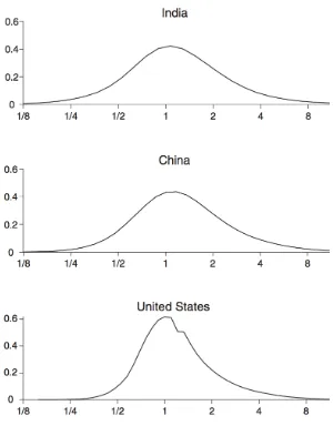
• Figure II plots the distribution of ln(TFPRsi/TFPRs) in US, China,

and India

• Normalized by industry average

• TFPR: dispersed a lot more in India and China than US

(44)

(45)

2.3 What industry characteristics

correlates w/ more variation in

TFPR?

• Run a regression of industry-level variance of ln(TFPRsi) on

industry-level covariates

• Those robustly correlated positively are:

• China: share of state-owned firms

• India: size restriction

(46)

China (Table XII)

(47)

2.4 Monopolistic competition

model

• How much productivity would go up if no distortion in India and China? • To answer this question, Hsieh &

(48)

Digression: Monopolistic competition

• 3 features (according to Matsuyama 1995)

• Each firm in an industry produces differentiated product and thus has monopoly power to set their output price

• With so many firms in each industry, each firm takes other firms’ behavior as given

ie. No strategic interactions as in oligopoly models

(49)

• Krugman (1980) applies this model to intl trade, to explain intra-industry trade

• Melitz (2003) also applies this model.

• Now the workhorse model of international trade

• Verhoogen (2008) & Bustos (2010) use this model to analyze plant-level data in Mexico / Argentine (& exploit natural experiments: currency

(50)

2.4.1 Model

• A representative final good

producer combines the outputs of S manufacturing industries by

(51)

• Each firm i in industry s produces differentiated products by

Ysi = AsiK_siαsL1_si−αs

• Their profits:

(1−τY_si)PsiYsi−wLsi −(1+τK_si)RKsi τYsi output distortions

• size restrictions, transportation costs, output subsidies

τKsi capital price distortions

(52)

2.4.2 Analysis

• Profit minimization w.r.t. Ysi by final

good producer implies:

Psi =

(53)

(54)

• FOCs for profit maximization of firm i give us the optimal level of inputs

Lsi =

• The demand curve equation PsiY

s is used to obtain

(55)

2.5 Gains from reallocation

• Industry TFP is expressed as: TFPs ≡

(56)

• Plug in the optimal level of Ksi and

Lsi. Then, lots of tweaks in algebra

• Use the demand curve equation for Psi.

• Treating Asi(1−τYsi)/(1+ τKsi)

α_s

as one term will help

(57)

• Now we need σ and Asi

• Use σ = 3

• Estimates in the literature ranges 3 to 10

• By using the demand curve equation, recoverYsi

(58)

• On the other hand, if no distortion, we have TFPRs = TFPRsi. Which

means

TFP_sefficient = � �

i

Aσ_si−1�σ−11

• Aggregating by Cobb-Douglas with

θs as each industry share, we can

(59)

Equalizing TFPR w/i industries raises TFP by (Table IV):

(60)

3. Other topics on firms in LDCs

• Contract enforcement

• McMillan & Woodruff (1999)

• Banerjee & Duflo (2000)

• Macchiavello & Morjaria (2010) • Impact of export

• Verhoogen (2008a)

• Bustos (2011)

(61)

Ashraf, Nava, James Berry, and Jesse M Shapiro. 2010.

“Can Higher Prices Stimulate Product Use? Evidence from

a Field Experiment in Zambia.”

American Economic

Review

100(5): 2383-2413.

Bandiera, Oriana, Iwan Barankay, and Imran Rasul. 2011.

“Field Experiments with Firms.”

Journal of Economic

Perspectives

25: 63-82.

Banerjee, Abhijit V., and Esther Duﬂo. 2000. “Reputation

Effects and the Limits of Contracting: A Study of the Indian

Software Industry.”

Quarterly Journal of Economics

115:

989-1017.

Banerjee, Abhijit V., and Esther Duﬂo. 2005. “Growth

Theory through the Lens of Development Economics.” In

Handbook of Economic Growth, eds. Philippe Aghion and

Steven N. Durlauf and Steven N. Durlauf. Elsevier, p.

473-552.

Besley, Timothy J., Konrad Burchardi, and Maitreesh

Ghatak. 2011. “Incentives and the de Soto Effect.”

Quarterly Journal of Economics

forthcoming.

Bustos, Paula. 2011. “Trade Liberalization, Exports, and

Technology Upgrading: Evidence on the Impact of

MERCOSUR on Argentinian Firms.”

American Economic

Review

101(1): 304-340.

de Mel, Suresh, David J. McKenzie, and Christopher

(62)

we ask how the sausage is made?”

Journal of Development

Economics

88(1): 19-31.

de Mel, Suresh, David McKenzie, and Christopher

Woodruff. 2010. “Returns to Capital in Microenterprises:

Evidence from a Field Experiment.”

Quarterly Journal of

Economics

123(4): 1329-1372.

Dupas, Pascaline, and Jonathan Robinson. 2009. “Savings

Constraints and Microenterprise Development: Evidence

from a Field Experiment in Kenya.”

National Bureau of

Economic Research Working Paper Series

No. 14693.

Keniston, Daniel. 2011. “Experimental vs. Structural

Estimates of the Return to Capital in Microenterprises.”

http://www.econ.yale.edu/conference/neudc11/papers/

paper_365.pdf.

Krugman, Paul. 1980. “Scale Economies, Product

Differentiation, and the Pattern of Trade.”

The American

Economic Review

70(5): 950-959.

Matsuyama, Kiminori. 1995. “Complementarities and

Cumulative Processes in Models of Monopolistic

Competition.”

Journal of Economic Literature

33(2):

701-729.

McKenzie, David. 2011. “How Can We Learn Whether

Firm Policies Are Working in Africa? Challenges (and

(63)