DOI 10.1007/s10640-009-9322-4
Is There a Win–Win Situation in Household Energy
Policy?
Bente Halvorsen · Bodil M. Larsen ·Runa Nesbakken
Accepted: 3 September 2009 / Published online: 19 September 2009 © Springer Science+Business Media B.V. 2009
Abstract To achieve environmental goals, most governments aim to reduce consumption of the most polluting energy goods by taxation. Often, the authorities not only aim to change the consumption of the regulated good by the taxation, but also to change the consumption of close substitutes (hereafter referred to as win–win effects). The size of the win–win effects depend not only on how close substitutes the goods are, but also on the price sensitivity of the taxed good and on the budget effects of the regulation. We use a conditional demand model to decompose the cross-price effect to discuss which criteria that must be fulfilled in order for substantial win–win effects to occur, using Norwegian stationary energy consumption as an empirical example.
Keywords Conditional demand model·Empirical microanalysis·
Residential energy demand·Separability test·Substitution
JEL Classification D12·Q41
1 Introduction
Reducing household energy consumption in order to reduce emissions has been a main tar-get for environmental policies in many countries. Often, when using a policy measure, the authorities not only aim to change the consumption of the regulated good, but also to change the consumption of close substitutes (hereafter referred to as win–win effects). In some cases, these win–win effects are an extra bonus of a particular policy. In other cases, the authorities
B. Halvorsen·B. M. Larsen (
B
)·R. NesbakkenStatistics Norway, P.O. Box 8131 Dep., 0033 Oslo, Norway e-mail: [email protected]; [email protected] B. Halvorsen
e-mail: [email protected] R. Nesbakken
may have to rely on these effects, as it is not possible or politically feasible to regulate the good of interest directly.
In practical policy making, these win–win effects are often assumed to be substantial and used actively as arguments for environmental policy. For example in the UK, the Government has announced plans to offer motorists subsidies of up to £ 5,000 to encourage them to buy electric or plug-in hybrid cars as part of a plan to promote low carbon transport over the next five years. Some policy actions are more local, as in the city of Oslo where electric cars are granted free parking, exemption from road tolls and permission to use the public transport lanes, and in Ontario Canada, where there is a proposal of CAD 10,000 subsidy for electric cars. Another Norwegian example of presumed win–win effects related to household stationary energy consumption is the discussion in the Norwegian national budgets of 1999 and 2000, where the government expresses concern of the effect on fuel oil consumption of an increase in the electricity taxes, proposing an increase in the fuel oil tax as well. It is also assumed that these tax increases will increase household consumption of biofuels, which is wanted in Norway to increase the consumption of renewable energy.
How efficient these cross good taxations are depends on the households’ substitution pos-sibilities in consumption, the price sensitivity of the regulated good as well as the budget effects of the regulation. If the goods are not used as substitutes in consumption, a win– win situation will not occur. For example, households may have different heating equipment using different types of energy in their residence. If two (or more) heating sources are used to heat the same area, the household may substitute one energy source for another. However, if the heating sources are installed in different rooms, the substitution possibilities are more limited. Likewise, the efficiency of policy measures aimed to increase the use of electric cars depend on how households actually use the electric cars; as an alternative to their petrol or diesel cars or as an alternative to public transportation or bicycling.
In order to evaluate the efficiency of cross subsidies/taxations, it is vital to analyse whether different energy sources are used as alternatives in consumption or if households use dif-ferent energy sources to produce difdif-ferent services (heating difdif-ferent rooms, driving shorter vs. longer distances). Furthermore, it is also important to know how other co-existing policy measures interact and affect demand response, and thus strengthen or weaken the win–win effects. For instance, it may be interesting to know why win–win effects are small, in order to carry out measures to increase the demand response, and thus strengthen the win–win effects.
This paper discusses the underlying demand structure behind win–win effects. We apply an empirical test for separability developed byBrowning and Meghir(1991), based onPollak (1969), using a conditional demand model.1The advantage of the conditional demand model is that it makes it possible to decompose the cross-price derivative into its ‘pure substitution’ and ‘money expenditure’ effects. The pure substitution effect consists of two components, of which one indicates if different energy carriers are separable, alternatives or complements in consumption, and the other one is the price sensitivity of the alternative good. The con-ditional demand models inPollak(1969) andBrowning and Meghir(1991) are based on cost functions. In this paper, we develop this model from the household utility maximization problem.
As an example, we look at policies aimed at reducing household electricity and fuel oil consumption and increasing household biofuel consumption, using a proposed increase in taxes on electricity and fuel oils for Norwegian households. We use the conditional demand
1 See alsoDeaton and Muellbauer(1980, pp. 127–128) for further information about the relation between
model to decompose the cross-price derivative of the biofuel consumption with respect to changes in the price of electricity and fuel oil, to discuss if we have a win–win situation in Norwegian household stationary energy consumption. We also discuss the possibilities to increase these effects, and how other policy measures aimed at reducing the environmental impacts on household energy consumption interact. The estimation of the conditional demand model is based on data from the Norwegian Survey of Consumer Expenditure (SCE).
2 Theoretical Foundation
In this section, we show the theoretical foundation for the conditional demand model and how a decomposition of the cross-price derivative can be used to evaluate how the demand structure affects the size of the win–win effects.
2.1 The Conditional Demand Function
We assume that households may use different energy carriers for space heating or to drive a particular distance; some may use one energy carrier, while others may use more than one depending on their capital stock. Assume further that the government want to increase (reduce) the use of one energy carrier (x1), called the good of interest, by increasing
(reduc-ing) the price of other energy carriers to reduce (increase) the consumption of alternative energy carriers (x2), hereafter referred to as conditioning goods. The consumption of these
energy carriers is decided simultaneously. The household is assumed to derive utility (U) from the consumption of bothx1 andx2, and from the consumption of other goods (x3),
given the characteristics of the household (a):
U=U(x1,x2,x3;a). (1)
We denote the corresponding prices of these goods as pi (i =1, 2, 3). The household is assumed to maximize utility subject to the budget constraint:Y−p1x1−p2x2−p3x3=0,
whereYis the household’s gross income. The maximization problem leads to the following first-order conditions:
Uxi′ −λpi =0, (2) whereλis the Lagrange multiplier for the budget constraint. To derive the conditional demand function, we solve all first-order conditions except one. Solving Eq.2fori=1 and 3 with respect toλ, we haveU
Y−p2x2is expenditure in excess of expenditures on energy carriers other thanx1.
Insert-ing the expression forx3into the demand forx1, and solving with respect tox1, gives the
conditional demand function for the good of interest:
x1=x1
In Eq.3, the demand forx1is conditional on the demand for other energy carriers (x2). The
demand for the good of interest is also conditional on a vector of household characteristics relevant to the consumption of goodx1,a1, containing demographic variables, e.g., age and
cars, etc.). Only durables that use the good of interest should be included ina1, because
the conditioning variable (x2) contains the effect of durables fed with type 2 energy on the
demand forx1. In optimum, this equals the conditional demand function defined byPollak
(1969),Browning and Meghir(1991) andDeaton and Muellbauer(1980). The conditional demand for the good of interest (x1) is a function of its own price, the prices of all goods
except the conditioning goods, total expenditure in excess of expenditure on the conditioning goods and the quantities of the conditioning goods.
Since only the price of the conditioning goods are assumed to change, the price of all other goods and services are normalized toonefor simplicity (p3 =1). Thus, we express
the conditional demand function for the good of interest as:
x1=x1(x2,p1,c−2;a1). (4)
2.2 Decomposition of the Cross-Price Derivative
Solving all first-order conditions with respect tox2, we obtain the ordinary (Marshallian)
demand function for x2 as a function of all prices (p), income (Y) and household
char-acteristics (a). Inserting this demand function forx2into the conditional demand function
for the good of interest given by Eq.4, we obtain the ordinary demand function for the good of interest as a function of all prices, income and household characteristics:x1 =
x1(x2(p,Y;a) ,p1,c−2;a1)=x1(p,Y;a). Using this property, the cross-price derivative
of the ordinary demand function for the good of interest is expressed by the derivatives of the conditional demand for the good of interest and the derivatives of the ordinary demand for the conditioning good. This is seen by differentiating Eq.4with respect top2, inserting
the ordinary demand function forx2and usingc−2=Y−p2x2:
ande22is the own-price Cournot elasticity forx2. The effect
on consumption ofx1due to an increase in p2(that is, the ordinary cross-price derivative) is
divided into two components. In Pollak’s terminology, the first term on the right-hand side in Eq.5is thepure substitution effect, and the second term is themoney expenditure effect. The pure substitution effect arises because an increase in the price of the conditioning good (p2) implies a change in demand for the conditioning good (x2). In turn, this causes a change
in consumption of the good of interest (x1). The money expenditure effect arises because an
increase in the price of the conditioning good implies a change in the level of expenditure for the non-conditioning goods(c−2), which in turn causes a change in the consumption of
the good of interest.2
2.3 Where Would We Expect Win–Win Effects?
Win–win effects occur when the cross-price derivative is large and positive. We may use this decomposition to evaluate under what circumstances win–win effects occur, and when
it is possible to regulate one good in order to achieve a target for another good. Looking at Eq.5, the pure substitution effect is negative if the goods in question are complements
∂x1 ∂x2 >0
and positive if they are alternatives∂x1 ∂x2 <0
, the pure substitution effect is negative if the goods are alternatives and positive if they are complements. The money expenditure effect will be negative if the own-price elasticity ofx2is less than one in absolute terms when
x1is a normal good∂c∂x−12 >0. Ifx1is inferior∂c∂x−12 <0or the own-price elasticity of the
conditioning good (e22)is larger than one in absolute terms, the money expenditure effect
is positive. Thus, both the pure substitution effect and the money expenditure effect may be negative or positive, and the total effect depends on the sign and magnitude of the two terms. In most cases,x1andx2 are substitutes in order for there to be any substantial win–win
effects of a policy instrument. The substitution effect is largest for close substitutes where the conditioning good is price sensitive (assuming thatx1is a normal good andx2is not a
Giffen good). In this case, the budget effect is negative, and small budget effects increase the win–win effects of a certain policy for a given substitution effect. For a given price sensitivity of the conditioning good (x2), the win–win effects are larger for strict necessity goods
com-pared to luxury goods. Thus, for a normal good, the win–win effects are highest for strong necessity goods where the alternative goods are close substitutes and where the conditioning good is very price sensitive.
With respect to energy policy making, we would expect to see win–win effects of a tax on electricity and fuel oil for space heating if the consumption of electricity and fuel oil is very price sensitive, the consumption of firewood is a strict necessity good, and if firewood and electricity and fuel oil are used to heat the same area (close substitutes). The share of households for which these conditions are met is also of great importance when evaluating the efficiency of cross policies for the entire population. The analogy for subsidizing the use of electric cars to reduce the use of fossil fuelled cars is that this policy will be efficient if the utilisation of electric cars is price sensitive, the consumption of fossil car fuel is a strict necessity good, and if electric and fossil fuelled cars are used to drive the same distance. However, if electric cars are likely to be used as a second car, mainly as a substitute to public transportation to drive shorter distances (within the city), the policy is less likely to be suc-cessful. The efficiency of this policy also depends on a sufficiently large share of households for which this is true.
3 Empirical Illustration
To illustrate how the conditional demand model may be used to shed light on various policy relevant issues related to the regulation of close substitutes, we apply the above model to discuss the existence of win–win effects of taxes on electricity and fuel oil with respect to household biofuel consumption.
3.1 Data
heating technology. With respect to stationary energy consumption, the SCE contain infor-mation about both the consumption and expenditures on fuel oils and biofuel, and electricity expenditures, during the last 12 months prior to the interview. In our data, firewood accounts for almost the entire household biofuel consumption.
Information about household electricity consumption from the electric utilities is applied. When this information is missing, we calculate electricity consumption by dividing the elec-tricity expenditures given in the SCE (net of the fixed amount) by the elecelec-tricity price. Information about the consumption of oil and firewood is taken directly from the SCE. Infor-mation on oil prices is collected from the Consumer Price Index (CPI) survey. The CPI survey includes monthly oil prices for most municipalities, which gives the variation in oil prices across households. When CPI data for a municipality are missing, average county-level prices are calculated using the CPI data and applied to households in that municipality. Firewood prices are calculated as the expenditure on firewood divided by the physical amount of firewood for households reporting both in the SCE. Average prices by municipality are then calculated and applied to all households in the municipality. Information on municipal electricity prices is from the Norwegian Water Resources and Energy Directorate. All prices, income and expenditures are indexed by the CPI, measuring monetary values in 1995 NOK.3 The Norwegian Institute of Meteorology provides annual information about regional varia-tions in temperature for municipalities.
The sample includes 3,958 households observed either in 1993, 1994 or 1995 using elec-tricity, firewood, fuel oil, or a combination of these for space heating. Heating systems based on more than one energy carrier are quite common. The share of households with heating equipment based on electricity in combination with equipment using fuel oil or firewood or both is 86% in our sample, while 14% have heating systems based on electricity only. We might thus expect to find substitution across energy carriers for space heating, indicat-ing that we may find substantial win–win effects in Norwegian household stationary energy consumption.
3.2 Econometric Specification
We now describe the econometric specification of the conditional demand function for bio-fuel (read firewood),x1in Eq.4, wherex2consists of fuel oil and electricity. We approximate
the conditional demand function for biofuel as:
BIO=α0+α1OIL+α2EL+α3PBIO+α4INC+
s
α5sHCs+u, (7)
whereBIOis the household’s total biofuel consumption measured in kWh,OILis household consumption of oil and kerosene,ELis household consumption of electricity,PBIOis the biofuel price andINCis household gross income less expenses for electricity and oil. The variablesOILandELare endogenous to the household. To avoid biased estimates, and to create the conditional demand function for biofuels, we estimate the instruments for these variables using predictions from the Marshallian demand functions for fuel oil and elec-tricity (see Eqs.8and9below).H Csare variables representing household characteristics, such as the amount of wood burning heating equipment, dummies for whether the household has a central heating system based on biofuels, the age and size of the dwelling, heating
3 If we interpret the CPI as an indication of the price on all other goods and services (p
3), the indexed prices
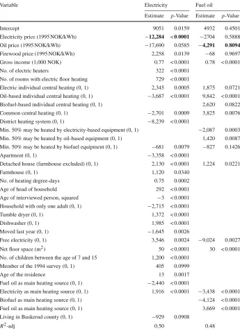
Table 1 Instrumental variable estimation for electricity and fuel oil consumption
Variable Electricity Fuel oil
Estimate p-Value Estimate p-Value
Intercept 9051 0.0159 4932 0.4501
Electricity price (1995 NOK/kWh) −12,284 <0.0001 −2704 0.5888
Oil price (1995 NOK/kWh) −17,690 0.0585 −4,291 0.8094
Firewood price (1995 NOK/kWh) 2,258 0.0139 −68 0.9697
Gross income (1,000 NOK) 0.77 < 0.0001 0.78 < 0.0001
No. of electric heaters 322 < 0.0001
No. of rooms with electric floor heating 729 < 0.0001
Electric individual central heating (0, 1) 2,345 0.0005 1,875 0.0721 Oil-based individual central heating (0, 1) −3,687 < 0.0001 9,842 < 0.0001 Biofuel-based individual central heating (0, 1) 2,620 0.0822
Common central heating (0, 1) −2,701 0.0009 3,825 0.0076
District heating system (0, 1) −8,239 < 0.0001
Min. 50% may be heated by electricity-based equipment (0, 1) −2,087 0.0003 Min. 50% may be heated by oil-based equipment (0, 1) 1,420 0.0087 Min. 50% may be heated by biofuel equipment (0, 1) −681 0.0079 −827 0.1426
Apartment (0, 1) −3,358 < 0.0001
Detached house (farmhouse excluded) (0, 1) 2,130 < 0.0001 1,224 0.0221
Farmhouse (0, 1) 1,120 0.0340
No. of heating degree-days 0.75 0.0002
Age of head of household 292 < 0.0001
Age of interviewed person, squared −3 < 0.0001 Household with only one adult (0, 1) −2,715 < 0.0001
Tumble dryer (0, 1) 1,372 < 0.0001
Dishwasher (0, 1) 1,985 < 0.0001
Moved last year (0, 1) −1,645 0.0026
Free electricity (0, 1) 3,546 0.0024 −9,024 0.0027
Net floor space (m2) 50 < 0.0001 30 < 0.0001
No. of children between the age of 7 and 15 1,200 < 0.0001
Member of the 1994 survey (0, 1) 405 0.0999
Age of the residence 13 0.0017
Fuel oil as main heating source (0, 1) −2,440 < 0.0001
Electricity as main heating source (0, 1) 1,916 < 0.0001 −3,438 < 0.0001
Biofuel as main heating source (0, 1) −4,124 < 0.0001
Fuel oil as main heating source (0, 1) 3,669 < 0.0001
Living in Buskerud county (0, 1) −929 0.0908
R2-adj 0.50 0.48
Note: Income and prices are in 1995 NOK. NOK1 is approximately USD 0.18
Coefficients printed in bold are parameters of particular interest for the size of the win-win effect
To decompose the cross-price derivative of the biofuel demand, we require estimates from the ordinary demand functions for fuel oil and electricity. These estimates are available from the instruments for the consumption of other energy carriers in the conditional demand func-tion for firewood. We approximate the ordinary demand funcfunc-tions (instruments) for fuel oil and electricity using:
wherePOILandPELare the prices of oil and electricity (normalized by the CPI), the vectors βandγ are parameters to be estimated andvandware stochastic error terms with similar characteristics as the error term in Eq.7.H Ckare household characteristics (see Table3for the list of variables).
3.3 Results
Table1provides the estimation results for instrument equations and Table2gives the estima-tion results for the condiestima-tional biofuel demand.4Coefficients printed in bold are parameters of particular interest when discussing the size of the win–win effect.
Looking at Table1, we see that electricity has a significant own price derivative whereas the own price effect on fuel oil consumption is not significant∂x2
∂p2 in Eq. 5
. Using the estimates in Table1and mean statistics, we calculated own price elasticities of−0.25 and
−0.81 for electricity and fuel oils, respectively (not shown in Table1). That is, we have a clear price effect for electricity, and a relatively large but uncertain price effect for fuel oils, which is due to the large heterogeneity in how households with fuel oil opportunities choose to utilise their equipment. We also see that we are able to identify a lot of heterogeneity in demand, in particular in the electricity consumption, and that approximately half of the variation in consumption of electricity and fuel oils are explained in these estimations.
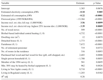
Looking at the results from the estimation of the conditional demand for firewood (see Table2) we see that both electricity and fuel oils can be regarded as substitutes to firewood in household energy consumption∂x1
∂x2 in Eq.5
, since the coefficients for the estimated elec-tricity and fuel oil consumption are negative. Both these parameters are significant, but the degree of actual substitution is not very large in this period. For instance, if the annual con-sumption of electricity is reduced by 100 kWh, the annual concon-sumption of firewood will only increase by 10 kWh (see the coefficient for the estimated electricity consumption in Table2). One reason is that electricity is not used for space heating only, but also for appliances, lighting, water heating, etc. Corrected for temperature variations, Norwegian households use approximately 30% of their electricity consumption for heating in this period. Furthermore, a large share of households with the opportunity to use firewood for space heating did not utilize their firewood equipment during these years. In our data, only 28% of the households with the opportunity to use firewood did have a positive expenditure on firewood. It is reason-able that the degree of substitution between firewood and electricity is higher for households who are actively using firewood for space heating. However, even if the level of substitution between electricity and firewood for space heating is considerable in this group, the overall level of substitution between electricity and firewood is still small because electricity is not only used for space heating and because not all households utilize their firewood stoves. For
Table 2 Estimated conditional residential demand for firewood, 1993–1995
Variable Estimate p-Value
Intercept 1,383 0.0676
Estimated electricity consumption, kWh −0.10 0.005
Estimated oil consumption, kWh −0.22 <0.0001
Firewood price (1995 NOK/kWh) −13,384 <0.0001
Income excl. est. elec./oil exp. (1,000 NOK) 3.56 0.0099
Income excl. est. electr./oil exp. highest 25% income dist. (1,000 NOK) −3.39 0.0009
No. of wood stoves 599 <0.0001
Biofuel-based individual central heating (1, 0) 4,732 <0.0001
Dwelling size(m2) 12 0.0079
Detached house (0, 1) 1,773 <0.0001
Farmhouse (0, 1) 7,672 <0.0001
No. of retirement pensioner 719 0.0372
No. of rooms in the residence 316 0.0093
Purchased fuel wood and fuel wood for free (gift, self-chopped, etc) 2,403 0.0008
Single-person household (0, 1) −1,788 0.0055
Member of the 1994 survey (0, 1) 581 0.0695
Min. 50% may be heated by biofuel equipment (0, 1) 962 0.0026
Living in Vest Agder county (0, 1) 9,718 <0.0001
Living in Rogaland county (0, 1) −1,203 0.0182
R2-adj 0.26
Note: Income and prices are in 1995 NOK. NOK1 is approximately USD 0.18
Coefficients printed in bold are parameters of particular interest for the size of the win-win effect
these reasons, electricity and firewood were not very close substitutes in household energy consumption in this period, and the effect of changes in firewood consumption as a result of reduced electricity consumption is, on average, relatively small.
With respect to the level of substitution in the consumption of fuel oils and firewood, a 100 kWh decrease in fuel oil consumption will only amount to a 22 kWh increase in firewood consumption (see the coefficient for the estimated fuel oil consumption in Table 2). Since all consumption of fuel oil is used for space heating in Norwegian households, this low figure implies that firewood and fuel oils are mainly used to heat different spaces of the residence, which limits the substitution possibilities.
Combining the own price sensitivity of the conditioning goods (presented in Table1) and the degree of substitution (presented in Table2) to calculate the entire substitution effect ∂x1
∂x2 ∂x2 ∂p2in Eq.5
, we find that the pure substitution effect from fuel oils are limited and uncer-tain, whereas the effect from the electricity consumption is much larger and less uncertain.
In addition to the pure substitution effect, the win–win effect depends on the income deriv-ative of the conditional demand function for firewood and on the own price elasticity and level of consumption of the conditioning good, which equal the derivative ofc−2with respect to
changes in the prise of the conditioning good∂x1 ∂c−2
∂c−2 ∂p2 in Eq.5
the income derivative is positive and significant for the rest of the income distribution (see Table2). The mean income derivative for the entire sample is very small, however, and will only increase mean consumption of firewood by 2 kWh (0.04% of firewood consumption) if income is increased by 1,000 NOK (0.3% of mean income excess of electricity and fuel oil expenditures). These small income derivatives makes the income effects almost negligible irrespective of the size of the own price derivatives and level of consumption. Thus, in this particular case, the win–win effects are mainly due to the pure substitution effects.
In our example, a increase in the electricity tax by 5 øre/kWh (11.5% of mean electricity price in the sample) will result in an estimated annual reduction of the electricity demand of 614 kWh (2.7% of mean annual electricity consumption in the sample) (see Table1), and an increase in fuel oil taxes by 5 øre/kWh will change the mean annual oil consumption by 215 kWh (11.8% of mean annual fuel oil consumption in the sample). These two tax changes will result in a total increase in mean firewood consumption by 18 kWh (0.4% of mean annual firewood consumption in the sample). Thus, even if many Norwegian households may use more than one energy source for space heating, increased electricity and fuel oil taxes will not have a major effect on household firewood consumption, indicating minor win–win effects.
4 The Relevance for Actual Policy Making
In real life, a particular policy measure will not only affect the consumption of a regu-lated good, but also the consumption of other close substitutes. Some of these effects are intended, others not. The conditional demand model may prove a useful tool when quantify-ing the effects (either intended or unintended) of various policy instruments on consumption. Mapping why and where a policy has undesired effects may also help policy makers to counterbalance these unwanted effects using other policy measures.
The main policy conclusion from the example above is that increasing taxes on electricity and fuel oil has a modest effect on household firewood consumption because the actual pure substitution effect between these goods is modest. This is again partly because many house-holds with the opportunity to consume firewood do not utilize this opportunity. One may also suspect that subsidizing the use of electric cars may not result in a substantial reduction in emissions from personal transportation. First, for those who have acquired an electric car, the majority use this as a second car, mainly because of its limited perimeter. This makes it more likely that it is used as a substitute to public transportation to drive shorter distances, as the long journeys must still be undertaken by conventional fossil fuelled cars. Second, the number of electric cars is very small, reducing the potential substantially. Both these reasons will reduce the substitution effect∂x1
∂x2
. The degree of actual substitution is probably higher for hybrid and hydrogen cars, but unless they constitute a sufficient share of the car fleet, the substitution effect will still be limited. It is, however, possible to implement policies in order to stimulate the purchase of these types of cars, regulate network externalities which lock households in the current car technology (sufficient number of fuelling stations, etc.), and to use policy measures to encourage households to use the more environmentally friendly transportation alternatives more often.
and pellets stoves. The aim of these policies is to increase the energy efficiency of the elec-tric heating equipment and to increase consumption of biofuels. As a result, a considerable amount of households have invested in heating pumps, of which the great majority of these are air to air pumps. Only a minor share of household has chosen to invest in pellets stoves. This policy of subsidizing investments in new heating technology has behavioural implica-tions. When electricity for space heating becomes more energy efficient, the real price of electricity for space heating is reduced (up to two thirds of the original price). This will make electricity for space heating relatively less expensive, changing the energy mix in the house-hold towards more use of electricity, reducing the share of biofuels and increasing the share of electricity, creating a conflict of interest. The reduction in real energy prices will also increase consumption opportunities for a given income (budget effect), leading to increased energy and other consumption. How large these effects are, is an empirical question. However, we cannot exclude the possibility that subsidizing more electricity efficient heating equipment may lead to increased electricity and reduced biofuel consumption without further analysis.
5 Conclusions
We have discussed a modelling framework for analysing the effects of cross good policy instruments. In many countries around the world, governments try to reduce the emissions from private transport by subsidising the purchase and use of electric and hybrid cars. In Norway, it has been an expressed political goal to reduce both domestic electricity and fuel oil consumption and increase biofuel consumption by increasing the electricity and fuel oil tax. How successful such cross good policy instruments are in achieving their goals, depend, in the short run, on whether households use these goods as alternatives in consumption and on the price sensitivity in the demand for the regulated goods.
In our example we find that the win–win effects are mainly driven by the pure substitution effect due to small negative budget effects. Our results show that electricity, fuel oil and fire-wood are indeed alternatives in consumption, indicating that households actually do switch between different energy carriers for space heating. Using the conditional demand model to decompose the cross-price effect, we have shown that the main reason why the win–win effects are limited in this example is that the degree of substitution is, on average, low. This is because electricity is used for many purposes and not all households with the opportunity to use firewood and fuel oils are using this opportunity. We have reason to believe that especially electricity and firewood for heating are almost perfect substitutes in some household groups. However, since these are few, the overall substitution effects are still limited. The analysis also indicates that other policy instruments, such as subsidizing heating pumps, may have a negative effect on household biofuel consumption. It is, however, an empirical question in each case whether the total effect of various policy measures is positive or negative.
Appendix
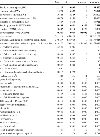
See Table3.
Table 3 Summary statistics for the sample, Norway 1993–1995
Mean SD Minimum Maximum
Electricity consumption, kWh 21,225 9,694 0 81,320
Oil consumption, kWh 1,894 6,055 0 70,397
Firewood consumption, kWh 3,744 8,549 0 159,600
Estimated electricity consumption, kWh 20,079 8,354 0 58,090
Estimated oil consumption, kWh 1,889 4,750 0 34,911
Electricity price (1995 NOK/kWh) 0.436 0.042 0.249 0.588
Oil price (1995 NOK/litre) 0.347 0.012 0.290 0.384
Firewood price (1995 NOK/kWh) 0.268 0.063 0.0002 0.446
Gross income 381,113 656,624 0 38,210,169
Income excl. estimated electricity/oil expenditures 370,459 655,960 0 38,173,015 Income excl. est. electr./oil exp. highest 25% income dist. 673,577 1,293,428 458,809 38,173,015
No. of electric heaters 5.043 3.105 0 30
No. of rooms with electric floor heating 1.475 1.901 0 12
No. of electric individual central heating 0.036 0.187 0 1
No. of stoves for oil/kerosene 0.134 0.364 0 3
No. of stoves for oil/kerosene and firewood 0.142 0.403 0 10
No. of oil-based individual central heating 0.037 0.188 0 1
No. of wood stoves 1.091 1.127 0 31
No. of firewood-based individual central heating 0.017 0.129 0 1
Dwelling size(m2) 128 56 11 600
Age of dwelling (years) 32 31 0 295
Apartment (0, 1) 0.102 0.303 0.000 1.000
Detached house (farmhouse excluded) (0, 1) 0.589 0.492 0.000 1.000
Farmhouse (0, 1) 0.092 0.289 0.000 1.000
No. of heating degree-days 4,149 588 3,284 6,277
No. of children (below 21 years) 0.964 1.124 0.000 7.000
Children aged 0–15 years (0, 1) 0.513 0.500 0.000 1.000
Single-person households (0, 1) 0.103 0.304 0.000 1.000
Oslo (0, 1) 0.082 0.274 0.000 1.000
Washing machine (0, 1) 0.948 0.223 0.000 1.000
Tumble dryer (0, 1) 0.464 0.499 0.000 1.000
Dishwasher (0, 1) 0.599 0.490 0.000 1.000
Moved last year (0, 1) 0.055 0.228 0.000 1.000
Free electricity (0, 1) 0.011 0.102 0.000 1.000
Age of interviewed person 45 14 17 88
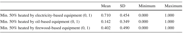
Table 3 continued
Mean SD Minimum Maximum
Min. 50% heated by electricity-based equipment (0, 1) 0.710 0.454 0.000 1.000 Min. 50% heated by oil-based equipment (0, 1) 0.142 0.349 0.000 1.000 Min. 50% heated by firewood-based equipment (0, 1) 0.402 0.490 0.000 1.000 3,958 observations
Coefficients printed in bold are parameters of particular interest for the size of the win-win effect
References
Browning M, Meghir C (1991) The effects of male and female labour supply on commodity demands. Eco-nometrica 59(4):925–951
Deaton A, Muellbauer J (1980) Economics and consumer behaviour. Cambridge University Press, Cambridge Pollak RA (1969) Conditional demand functions and consumption theory. Q J Econ 83(1):60–78