Abul Hasan Siddiqi
Functional
Editor-in-chief
Abul Hasan Siddiqi, Sharda University, Greater Noida, India Editorial Board
Zafer Aslan, International Centre for Theoretical Physics, Istanbul, Turkey M. Brokate, Technical University, Munich, Germany
N.K. Gupta, Indian Institute of Technology Delhi, New Delhi, India
Akhtar Khan, Center for Applied and Computational Mathematics, Rochester, USA Rene Lozi, University of Nice Sophia-Antipolis, Nice, France
monographs, lecture notes and contributed volumes focusing on areas where mathematics is used in a fundamental way, such as industrial mathematics, bio-mathematics,financial mathematics, applied statistics, operations research and computer science.
Functional Analysis
and Applications
School of Basic Sciences and Research Sharda University
Greater Noida, Uttar Pradesh India
ISSN 2364-6837 ISSN 2364-6845 (electronic) Industrial and Applied Mathematics
ISBN 978-981-10-3724-5 ISBN 978-981-10-3725-2 (eBook) https://doi.org/10.1007/978-981-10-3725-2
Library of Congress Control Number: 2018935211 ©Springer Nature Singapore Pte Ltd. 2018
This work is subject to copyright. All rights are reserved by the Publisher, whether the whole or part of the material is concerned, specifically the rights of translation, reprinting, reuse of illustrations, recitation, broadcasting, reproduction on microfilms or in any other physical way, and transmission or information storage and retrieval, electronic adaptation, computer software, or by similar or dissimilar methodology now known or hereafter developed.
The use of general descriptive names, registered names, trademarks, service marks, etc. in this publication does not imply, even in the absence of a specific statement, that such names are exempt from the relevant protective laws and regulations and therefore free for general use.
The publisher, the authors and the editors are safe to assume that the advice and information in this book are believed to be true and accurate at the date of publication. Neither the publisher nor the authors or the editors give a warranty, express or implied, with respect to the material contained herein or for any errors or omissions that may have been made. The publisher remains neutral with regard to jurisdictional claims in published maps and institutional affiliations.
Printed on acid-free paper
This Springer imprint is published by the registered company Springer Nature Singapore Pte Ltd. part of Springer Nature
Functional analysis was invented and developed in the twentieth century. Besides being an area of independent mathematical interest, it provides many fundamental notions essential for modeling, analysis, numerical approximation, and computer simulation processes of real-world problems. As science and technology are increasingly refined and interconnected, the demand for advanced mathematics beyond the basic vector algebra and differential and integral calculus has greatly increased. There is no dispute on the relevance of functional analysis; however, there have been differences of opinion among experts about the level and methodology of teaching functional analysis. In the recent past, its applied nature has been gaining ground.
The main objective of this book is to present all those results of functional analysis, which have been frequently applied in emerging areas of science and technology.
Functional analysis provides basic tools and foundation for areas of vital importance such as optimization, boundary value problems, modeling real-world phenomena, finite and boundary element methods, variational equations and inequalities, inverse problems, and wavelet and Gabor analysis. Wavelets, formally invented in the mid-eighties, have found significant applications in image pro-cessing and partial differential equations. Gabor analysis was introduced in 1946, gaining popularity since the last decade among the signal processing community and mathematicians.
The book comprises 15 chapters, an appendix, and a comprehensive updated bibliography. Chapter1is devoted to basic results of metric spaces, especially an importantfixed-point theorem called the Banach contraction mapping theorem, and its applications to matrix, integral, and differential equations. Chapter2deals with basic definitions and examples related to Banach spaces and operators defined on such spaces. A sufficient number of examples are presented to make the ideas clear. Algebras of operators and properties of convex functionals are discussed. Hilbert space, an infinite-dimensional analogue of Euclidean space offinite dimension, is introduced and discussed in detail in Chap.3. In addition, important results such as projection theorem, Riesz representation theorem, properties of self-adjoint,
positive, normal, and unitary operators, relationship between bounded linear operator and bounded bilinear form, and Lax–Milgram lemma dealing with the existence of solutions of abstract variational problems are presented. Applications and generalizations of the Lax–Milgram lemma are discussed in Chaps.7 and 8. Chapter 4 is devoted to the Hahn–Banach theorem, Banach–Alaoglu theorem, uniform boundedness principle, open mapping, and closed graph theorems along with the concept of weak convergence and weak topologies. Chapter5provides an extension of finite-dimensional classical calculus to infinite-dimensional spaces, which is essential to understand and interpret various current developments of science and technology. More precisely, derivatives in the sense of Gâteau, Fréchet, Clarke (subgradient), and Schwartz (distributional derivative) along with Sobolev spaces are the main themes of this chapter. Fundamental results concerning exis-tence and uniqueness of solutions and algorithm for finding solutions of opti-mization problems are described in Chap.6. Variational formulation and existence of solutions of boundary value problems representing physical phenomena are described in Chap.7. Galerkin and Ritz approximation methods are also included. Finite element and boundary element methods are introduced and several theorems concerning error estimation and convergence are proved in Chap.8. Chapter 9is devoted to variational inequalities. A comprehensive account of this elegant mathematical model in terms of operators is given. Apart from existence and uniqueness of solutions, error estimation andfinite element methods for approxi-mate solutions and parallel algorithms are discussed. The chapter is mainly based on the work of one of its inventors, J. L. Lions, and his co-workers and research students. Activities at the Stampacchia School of Mathematics, Erice, Italy, are providing impetus to researchers in thisfield. Chapter10is devoted to rudiments of spectral theory with applications to inverse problems. We present frame and basis theory in Hilbert spaces in Chap. 11. Chapter 12 deals with wavelets. Broadly, wavelet analysis is a refinement of Fourier analysis and has attracted the attention of researchers in mathematics, physics, and engineering alike. Replacement of the classical Fourier methods, wherever they have been applied, by emerging wavelet methods has resulted in drastic improvements. In this chapter, a detailed account of this exciting theory is presented. Chapter13presents an introduction to applications of wavelet methods to partial differential equations and image processing. These are emerging areas of current interest. There is still a wide scope for further research. Models and algorithms for removal of an unwanted component (noise) of a signal are discussed in detail. Error estimation of a given image with its wavelet repre-sentation in the Besov norm is given. Wavelet frames are comparatively a new addition to wavelet theory. We discuss their basic properties in Chap.14. Dennis Gabor, Nobel Laureate of Physics (1971), introduced windowed Fourier analysis, now called Gabor analysis, in 1946. Fundamental concepts of this analysis with certain applications are presented in Chap.15.
The book is self-contained and provides examples, updated references, and applications in diverse fields. Several problems are thought-provoking, and many lead to new results and applications. The book is intended to be a textbook for graduate or senior undergraduate students in mathematics. It could also be used for an advance course in system engineering, electrical engineering, computer engi-neering, and management sciences. The proofs of theorems and other items marked with an asterisk may be omitted for a senior undergraduate course or a course in other disciplines. Those who are mainly interested in applications of wavelets and Gabor system may study Chaps.2,3, and11to15. Readers interested in variational inequalities and its applications may pursue Chaps.3,8, and9. In brief, this book is a handy manual of contemporary analytic and numerical methods in infinite-dimensional spaces, particularly Hilbert spaces.
I have used a major part of the material presented in the book while teaching at various universities of the world. I have also incorporated in this book the ideas that emerged after discussion with some senior mathematicians including Prof. M. Z. Nashed, Central Florida University; Prof. P. L. Butzer, Aachen Technical University; Prof. Jochim Zowe and Prof. Michael Kovara, Erlangen University; and Prof. Martin Brokate, Technical University, Munich.
I take this opportunity to thank Prof. P. Manchanda, Chairperson, Department of Mathematics, Guru Nanak Dev University, Amritsar, India; Prof. Rashmi Bhardwaj, Chairperson, Non-linear Dynamics Research Lab, Guru Gobind Singh Indraprastha University, Delhi, India; and Prof. Q. H. Ansari, AMU/KFUPM, for their valuable suggestions in editing the manuscript. I also express my sincere thanks to Prof. M. Al-Gebeily, Prof. S. Messaoudi, Prof. K. M. Furati, and Prof. A. R. Khan for reading carefully different parts of the book.
1 Banach Contraction Fixed Point Theorem . . . 1
1.1 Objective . . . 1
1.2 Contraction Fixed Point Theorem by Stefan Banach . . . 1
1.3 Application of Banach Contraction Mapping Theorem . . . 7
1.3.1 Application to Matrix Equation. . . 7
1.3.2 Application to Integral Equation . . . 9
1.3.3 Existence of Solution of Differential Equation . . . 12
1.4 Problems . . . 13
2 Banach Spaces . . . 15
2.1 Introduction . . . 15
2.2 Basic Results of Banach Spaces. . . 16
2.2.1 Examples of Normed and Banach Spaces . . . 17
2.3 Closed, Denseness, and Separability. . . 20
2.3.1 Introduction to Closed, Dense, and Separable Sets. . . . 20
2.3.2 Riesz Theorem and Construction of a New Banach Space . . . 22
2.3.3 Dimension of Normed Spaces. . . 22
2.3.4 Open and Closed Spheres. . . 23
2.4 Bounded and Unbounded Operators. . . 25
2.4.1 Definitions and Examples. . . 25
2.4.2 Properties of Linear Operators. . . 33
2.4.3 Unbounded Operators. . . 40
2.5 Representation of Bounded and Linear Functionals. . . 41
2.6 Space of Operators . . . 43
2.7 Convex Functionals . . . 48
2.7.1 Convex Sets. . . 48
2.7.2 Affine Operator . . . 50
2.7.3 Lower Semicontinuous and Upper Semicontinuous Functionals . . . 53
2.8 Problems . . . 54
2.8.1 Solved Problems . . . 54
2.8.2 Unsolved Problems. . . 65
3 Hilbert Spaces. . . 71
3.1 Introduction . . . 71
3.2 Fundamental Definitions and Properties . . . 72
3.2.1 Definitions, Examples, and Properties of Inner Product Space . . . 72
3.2.2 Parallelogram Law . . . 78
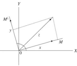
3.3 Orthogonal Complements and Projection Theorem . . . 80
3.3.1 Orthogonal Complements and Projections . . . 80
3.4 Orthogonal Projections and Projection Theorem . . . 83
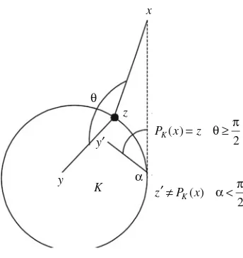
3.5 Projection on Convex Sets . . . 90
3.6 Orthonormal Systems and Fourier Expansion . . . 93
3.7 Duality and Reflexivity. . . 101
3.7.1 Riesz Representation Theorem . . . 101
3.7.2 Reflexivity of Hilbert Spaces. . . 105
3.8 Operators in Hilbert Space . . . 106
3.8.1 Adjoint of Bounded Linear Operators on a Hilbert Space . . . 106
3.8.2 Self-adjoint, Positive, Normal, and Unitary Operators. . . 112
3.8.3 Adjoint of an Unbounded Linear Operator. . . 121
3.9 Bilinear Forms and Lax–Milgram Lemma . . . 123
3.9.1 Basic Properties. . . 123
3.10 Problems . . . 132
3.10.1 Solved Problems . . . 132
3.10.2 Unsolved Problems. . . 140
4 Fundamental Theorems . . . 145
4.1 Introduction . . . 145
4.2 Hahn–Banach Theorem. . . 146
4.3 Topologies on Normed Spaces. . . 155
4.3.1 Compactness in Normed Spaces . . . 155
4.3.2 Strong and Weak Topologies . . . 157
4.4 Weak Convergence. . . 158
4.4.1 Weak Convergence in Banach Spaces . . . 158
4.4.2 Weak Convergence in Hilbert Spaces . . . 161
4.5 Banach–Alaoglu Theorem. . . 164
4.6 Principle of Uniform Boundedness and Its Applications . . . 166
4.6.1 Principle of Uniform Boundedness . . . 166
4.7 Open Mapping and Closed Graph Theorems . . . 167
4.7.2 Open Mapping Theorem. . . 170
4.7.3 The Closed Graph Theorem . . . 171
4.8 Problems . . . 171
4.8.1 Solved Problems . . . 171
4.8.2 Unsolved Problems. . . 175
5 Differential and Integral Calculus in Banach Spaces. . . 177
5.1 Introduction . . . 177
5.2 The Gâteaux and Fréchet Derivatives. . . . 178
5.2.1 The Gâteaux Derivative . . . . 178
5.2.2 The Fréchet Derivative. . . . 182
5.3 Generalized Gradient (Subdifferential) . . . 190
5.4 Some Basic Results from Distribution Theory and Sobolev Spaces . . . 192
5.4.1 Distributions . . . 192
5.4.2 Sobolev Space . . . 206
5.4.3 The Sobolev Embedding Theorems. . . 211
5.5 Integration in Banach Spaces. . . 215
5.6 Problems . . . 218
5.6.1 Solved Problems . . . 218
5.6.2 Unsolved Problems. . . 223
6 Optimization Problems . . . 227
6.1 Introduction . . . 227
6.2 General Results on Optimization . . . 227
6.3 Special Classes of Optimization Problems . . . 231
6.3.1 Convex, Quadratic, and Linear Programming. . . 231
6.3.2 Calculus of Variations and Euler–Lagrange Equation . . . 231
6.3.3 Minimization of Energy Functional (Quadratic Functional). . . 233
6.4 Algorithmic Optimization . . . 234
6.4.1 Newton Algorithm and Its Generalization . . . 234
6.4.2 Conjugate Gradient Method . . . 243
6.5 Problems . . . 246
7 Operator Equations and Variational Methods . . . 249
7.1 Introduction . . . 249
7.2 Boundary Value Problems. . . 249
7.3 Operator Equations and Solvability Conditions. . . 253
7.3.1 Equivalence of Operator Equation and Minimization Problem. . . 253
7.3.2 Solvability Conditions . . . 255
7.4 Existence of Solutions of Dirichlet and Neumann Boundary
Value Problems . . . 259
7.5 Approximation Method for Operator Equations. . . 263
7.5.1 Galerkin Method . . . 263
7.5.2 Rayleigh–Ritz–Galerkin Method . . . 266
7.6 Eigenvalue Problems. . . 267
7.6.1 Eigenvalue of Bilinear Form. . . 267
7.6.2 Existence and Uniqueness. . . 268
7.7 Boundary Value Problems in Science and Technology . . . 269
7.8 Problems . . . 274
8 Finite Element and Boundary Element Methods. . . 277
8.1 Introduction . . . 277
8.2 Finite Element Method . . . 280
8.2.1 Abstract Problem and Error Estimation . . . 280
8.2.2 Internal Approximation ofH1ðXÞ . . . 286
8.2.3 Finite Elements . . . 287
8.3 Applications of the Finite Method in Solving Boundary Value Problems . . . 292
8.4 Introduction of Boundary Element Method. . . 297
8.4.1 Weighted Residuals Method . . . 297
8.4.2 Boundary Solutions and Inverse Problem. . . 299
8.4.3 Boundary Element Method . . . 301
8.5 Problems . . . 307
9 Variational Inequalities and Applications . . . 311
9.1 Motivation and Historical Remarks . . . 311
9.1.1 Contact Problem (Signorini Problem) . . . 311
9.1.2 Modeling in Social, Financial and Management Sciences. . . 312
9.2 Variational Inequalities and Their Relationship with Other Problems. . . 313
9.2.1 Classes of Variational Inequalities. . . 313
9.2.2 Formulation of a Few Problems in Terms of Variational Inequalities. . . 315
9.3 Elliptic Variational Inequalities . . . 320
9.3.1 Lions–Stampacchia Theorem. . . 321
9.3.2 Variational Inequalities for Monotone Operators. . . 323
9.4 Finite Element Methods for Variational Inequalities . . . 329
9.4.1 Convergence and Error Estimation . . . 329
9.4.2 Error Estimation in Concrete Cases. . . 333
9.5 Evolution Variational Inequalities and Parallel Algorithms . . . . 335
9.5.1 Solution of Evolution Variational Inequalities . . . 335
9.6 Obstacle Problem . . . 345
9.6.1 Obstacle Problem. . . 345
9.6.2 Membrane Problem (Equilibrium of an Elastic Membrane Lying over an Obstacle). . . 346
9.7 Problems . . . 348
10 Spectral Theory with Applications . . . 351
10.1 The Spectrum of Linear Operators. . . 351
10.2 Resolvent Set of a Closed Linear Operator. . . 355
10.3 Compact Operators. . . 356
10.4 The Spectrum of a Compact Linear Operator . . . 360
10.5 The Resolvent of a Compact Linear Operator. . . 361
10.6 Spectral Theorem for Self-adjoint Compact Operators. . . 363
10.7 Inverse Problems and Self-adjoint Compact Operators. . . 368
10.7.1 Introduction to Inverse Problems. . . 368
10.7.2 Singular Value Decomposition . . . 370
10.7.3 Regularization . . . 373
10.8 Morozov’s Discrepancy Principle. . . 377
10.9 Problems . . . 380
11 Frame and Basis Theory in Hilbert Spaces. . . 381
11.1 Frame in Finite-Dimensional Hilbert Spaces. . . 381
11.2 Bases in Hilbert Spaces. . . 386
11.2.1 Bases. . . 386
11.3 Riesz Bases . . . 389
11.4 Frames in Infinite-Dimensional Hilbert Spaces . . . 391
11.5 Problems . . . 394
12 Wavelet Theory. . . 399
12.1 Introduction . . . 399
12.2 Continuous and Discrete Wavelet Transforms. . . 400
12.2.1 Continuous Wavelet Transforms . . . 400
12.2.2 Discrete Wavelet Transform and Wavelet Series . . . 409
12.3 Multiresolution Analysis, and Wavelets Decomposition and Reconstruction . . . 415
12.3.1 Multiresolution Analysis (MRA). . . 415
12.3.2 Decomposition and Reconstruction Algorithms . . . 418
12.3.3 Wavelets and Signal Processing . . . 421
12.3.4 The Fast Wavelet Transform Algorithm. . . 423
12.4 Wavelets and Smoothness of Functions . . . 425
12.4.1 Lipschitz Class and Wavelets . . . 425
12.4.2 Approximation and Detail Operators . . . 429
12.4.3 Scaling and Wavelet Filters. . . 435
12.5 Compactly Supported Wavelets . . . 446
12.5.1 Daubechies Wavelets . . . 446
12.5.2 Approximation by Families of Daubechies Wavelets . . . 452
12.6 Wavelet Packets . . . 460
12.7 Problems . . . 461
13 Wavelet Method for Partial Differential Equations and Image Processing. . . 465
13.1 Introduction . . . 465
13.2 Wavelet Methods in Partial Differential and Integral Equations. . . 466
13.2.1 Introduction. . . 466
13.2.2 General Procedure . . . 467
13.2.3 Miscellaneous Examples. . . 471
13.2.4 Error Estimation Using Wavelet Basis. . . 476
13.3 Introduction to Signal and Image Processing . . . 479
13.4 Representation of Signals by Frames . . . 480
13.4.1 Functional Analytic Formulation. . . 480
13.4.2 Iterative Reconstruction . . . 482
13.5 Noise Removal from Signals. . . 484
13.5.1 Introduction. . . 484
13.5.2 Model and Algorithm. . . 486
13.6 Wavelet Methods for Image Processing . . . 489
13.6.1 Besov Space . . . 489
13.6.2 Linear and Nonlinear Image Compression . . . 491
13.7 Problems . . . 493
14 Wavelet Frames . . . 497
14.1 General Wavelet Frames. . . 497
14.2 Dyadic Wavelet Frames . . . 502
14.3 Frame Multiresolution Analysis. . . 506
14.4 Problems . . . 508
15 Gabor Analysis. . . 509
15.1 Orthonormal Gabor System. . . 509
15.2 Gabor Frames. . . 511
15.3 HRT Conjecture for Wave Packets . . . 517
15.4 Applications. . . 518
Appendix. . . 521
References. . . 549
Index . . . 557
Abul Hasan Siddiqi is a distinguished scientist and professor emeritus at the School of Basic Sciences and Research, Sharda University, Greater Noida, India. He has held several important administrative positions such as Chairman, Department of Mathematics; Dean Faculty of Science; Pro-Vice-Chancellor of Aligarh Muslim University. He has been actively associated with International Centre for Theoretical Physics, Trieste, Italy (UNESCO’s organization), in different capacities for more than 20 years; was Professor of Mathematics at King Fahd University of Petroleum and Minerals, Saudi Arabia, for 10 years; and was Consultant to Sultan Qaboos University, Oman, for five terms, Istanbul Aydin University, Turkey, for 3 years, and the Institute of Micro-electronics, Malaysia, for 5 months. Having been awarded three German Academic Exchange Fellowships to carry out mathematical research in Germany, he has also jointly published more than 100 research papers with his research collaborators andfive books and edited proceedings of nine international conferences. He is the Founder Secretary of the Indian Society of Industrial and Applied Mathematics (ISIAM), which celebrated its silver jubilee in January 2016. He is editor-in-chief of the Indian Journal of Industrial and Applied Mathematics, published by ISIAM, and of the Springer’s book series Industrial and Applied Mathematics. Recently, he has been elected President of ISIAM which represents India at the apex forum of industrial and applied mathematics—ICIAM.
Banach Contraction Fixed Point
Theorem
Abstract The main goal of this chapter is to introduce notion of distance between two points in an abstract set. This concept was studied by M. Fréchet and it is known as metric space. Existence of a fixed point of a mapping on a complete metric space into itself was proved by S. Banach around 1920. Application of this theorem for existence of matrix, differential and integral equations is presented in this chapter. Keywords Metric space
·
Complete metric space·
Fixed point·
Contraction mapping·
Hausdorff metric1.1
Objective
The prime goal of this chapter is to discuss the existence and uniqueness of a fixed point of a special type of mapping defined on a metric space into itself, called con-traction mapping along with applications.
1.2
Contraction Fixed Point Theorem by Stefan Banach
Definition 1.1 Let
d(·,·): X×X → R
be a real-valued function on X×X, where X is a nonempty set.d(·,·)is called a metricand(X,d)is called ametric spaceifd(·,·)satisfies the following conditions: 1. d(x,y)≥0∀x,y∈ X,d(x,y)=0 if and only ifx=y.
2. d(x,y)=d(y,x)for allx,y∈ X,
3. d(x,y)≤d(x,z)+d(z,y)for allx,y,z∈ X.
Remark 1.1 d(x,y)is also known as thedistancebetweenxandybelonging to X. It is a generalization of the distance between two points on real line.
© Springer Nature Singapore Pte Ltd. 2018
A. H. Siddiqi,Functional Analysis and Applications, Industrial and Applied Mathematics, https://doi.org/10.1007/978-981-10-3725-2_1
It may be noted that positivity condition:
d(x,y)≥0∀x,y∈X
follows from second part of condition (i).d(x,y) ≤ d(x,z)+d(z,y)by(i i i). Choosingx=y, we get:
d(x,x)≤d(x,z)+d(z,x)or 0≤2d(x,z)forx,z∈ X because
d(x,x)=0 andd(x,z)=d(z,x).
Hence for allx,z∈X,d(x,z)≥0, namely positivity.
Remark 1.2 A subsetY of a metric space(X,d)is itself a metric space.(Y,d)is a metric space ifY ⊆Xand
d1(x,y)=d(x,y)∀x,y∈Y Examples of Metric Spaces
Example 1.1 Let
d(·,·): R×R→ R (1.1)
be defined by
d(x,y)= |x−y| ∀x,y∈ R.
Thend(·,·)is a metric onR(distance between two points of R) and(R,d)is a metric space.
Example 1.2 Let R2 denote the Euclidean space of dimension 2. Define a func-tion d(·,·) on R2 as follows: d(x,y) = ((u
1 − u2)2 +(v1 −v2)2)1/2, where x=(u1,u2),y=(v1,v2).
d(·,·)is a metric onR2and(R2,d)is a metric space,
Example 1.3 LetRndenote the vector space of dimension n. Foru =(u1,u2, . . . , un)∈ Rn andv=(v1,v2, . . . ,vn)∈ Rn. Defined(·,·)as follows:
(a) d(u,v)=( n k=1
|uk−vk|2)1/2. (Rn,d)is a metric space.
Example 1.4 For a number p satisfying 1 ≤ p < ∞, letℓp denote the space of infinite sequencesu=(u1,u2, . . . ,un, ..)such that the series
∞ k=1
d(u,v)= ∞
k=1
|uk−vk|p 1/p
,
u =(u1,u2, . . . ,uk, ..),v=(v1,v2, . . . ,vk, ..)∈ℓp. d(·,·)is distance between elements ofℓp.
Example 1.5 SupposeC[a,b] represents the set of all real continuous functions defined on closed interval[a,b]. Letd(·,·)be a function defined onC[a,b]×C[a,b] by:
(a) d(f,g)= sup a≤x≤b
|f(x)−g(x)|,∀ f,g∈C[a,b]
(b) d(f,g)=
b a
|f(x)−g(x)|2dx 1/2
, ∀ f,g ∈C[a,b].
(C[a,b],d(·,·))is a metric space with respect to metrices given in(a)and(b). Example 1.6 SupposeL2[a,b]denote the set of all integrable functions f defined on[a,b]such that
b lim
a |f|
2d xis finite. Then,(L
2[a,b],d(·,·))is a metric space if
d(f,g)=( b a
|f(x)−g(x)|2dx)1/2, f,g∈ L2[a,b]
d(·,·)is a metric onL2[a,b].
Definition 1.2 Let{un}be a sequence of points in a metric space(X,d)which is called aCauchy sequenceif for everyε >0, there is an integer Nsuch that
d(um,un) < ε∀n,m>N.
It may be recalled that a sequence in a metric space is a function having domain as the set of natural numbers and the range as a subset of the metric space. The definition of Cauchy sequence means that the distance between two pointsunandumis very small whennandmare very large.
Definition 1.3 Let{un}be a sequence in a metric space(X,d). It is calledconvergent with limituin X if, forε >0, there exists a natural number Nhaving property
d(un,u) < ε∀n>N
If{un}converges to u, that is,{un} →uasn → ∞, then we write, lim
Complete Metric Spaces
Example 1.7 (a) SpacesR,R2,Rn, ℓ
p,C[a,b]with metric(a)of Example1.5and L2[a,b]are examples of complete metric spaces.
(b) (0,1]is not a complete metric space.
(c) C[a,b]with integral metric is not a complete metric space. (d) The set of rational numbers is not a complete metric space. (e) C[a,b]with (b) of Example1.5is not complete metric space.
Definition 1.5 (a) A subsetM of a metric space(X,d)is said to bebounded if there exists a positive constantksuch thatd(u,v)≤kfor allu,vbelonging to M.
(b) A subsetMof a metric space(X,d)isclosedif every convergent sequence{un} inM is convergent inM.
(c) If every bounded sequenceM ⊂(X,d)has a convergent subsequence then the subset M is calledcompact.
(d) LetT :(X,d)→(Y,d). T is calledcontinuousifun →uimplies thatT(un)→ T u; that is,d(un,u)→0 asn→ ∞implies thatd(T(un),T u)→0.
Remark 1.3 1. It may be noted that every bounded and closed subset of(Rn,d)is a compact subset.
2. It may be observed that each closed subset of a complete metric space is complete. As we see above, a metric is a distance between two points. We introduce now the concept of distance between the subsets of a set, for example, distance between a line and a circle inR2. This is called Hausdorff metric.
Distance Between Two Subsets (Hausdorff Metric)
LetX be a set andH(X)be a set of all subsets ofX. Supposed(·,·)be a metric on X. Then distance between a pointuofX and a subset M of X is defined as
d(u,M)=inf{d(u,v)/v∈M} or = inf
v∈M{d(u,v)}
Let M and N be two elements ofH(X). Distance or metric between M and N denoted by (M,N) is defined as
d(M,N)=sup u∈M
inf v∈Nd(u,v) =sup
u∈M
d(u,N).
It can be verified that
where
d(N,M)=sup v∈N
inf u∈Md(v,u) =sup
u∈M inf
u∈Nd(u,v).
Definition 1.6 The Hausdorff metric or the distance between two elementsMand N of a metric(X,d), denoted byh(M,N), is defined as
h(M,N)=max{d(M,N),d(N,M)}
Remark 1.4 IfH(X)denotes the set of all closed and bounded subsets of a metric space(X,d)thenh(M,N)is a metric. IfX =R2thenH(R2)the set of all compact subsets of R2is a metric space with respect toh(M,N).
Contraction Mapping
Definition 1.7 (Contraction Mapping) A mappingT :(X,d)→(X,d)is called a Lipschitz continuous mappingif there exists a numberαsuch that
d(T u,T v)≤αd(u,v)∀u,v∈ X.
Ifαlies in[0,1), that is, 0 ≤α <1, thenT is called acontraction mapping.αis called the contractivity factor ofT.
Example 1.8 LetT: R→ Rbe defined asT u=(1+u)1/3. Then finding a solution to the equationT u=uis equivalent to solving the equationu3−u−1=0.T is a contraction mapping onI = [1,2], where the contractivity factor isα=(3)1/3−1. Example 1.9 (a) LetT u=1/3u,0≤u ≤1. ThenT is a contraction mapping on
[0,1]with contractivity factor 1/3.
(b) Let S(u) =u +b, u ∈ R andb be any fixed element of R. Then S is not a contraction mapping.
Example 1.10 LetI = [a,b]and f: [a,b] → [a,b]and suppose that f′(u)exist and|f′(x)|<1. Then f is a contraction mapping onI into itself.
Definition 1.8 (Fixed Point) LetTbe a mapping on a metric space(X,d)into itself. u ∈X is called a fixed point if
T u=u
such that T u=u, that T has a unique fixed point. Furthermore, for any u∈(X,d), the sequence x,T(x),T2(x), . . . ,Tk(x)converges to the point u; that is
lim k→∞T
k=u
Proof We know thatT2(x)=T(T(x)), . . . ,Tk(x)=T(T(k−1)(x)), and d(Tm(x),Tn(x))≤αd(Tm−1(x),T(n−1)(x))
≤αmd(x,Tn−m(x)) ≤αm
n−m k=1
d(Tk−1(x),Tk(x))
≤αm n−m k=1
αk−1d(x,T(x))
This we obtain by applying contractivity(k−1)times. It is clear that d(Tm(x),Tn(x))→0as m,n→ ∞
and soTm(x)is a Cauchy sequence in a complete metric space(X,d). This sequence must be convergent, that is
lim m→∞T
mx=u
We show thatuis a fixed point ofT, that is,T(u)=u. In fact, we will show thatu is unique.T(u)=uis equivalent to showing thatd(T(u),u)=0.
d(T(u),u)=d(u,T(u))
≤d(u,Tk(x))+d(Tk(x),T(u))
≤d(u,Tk(x))+αd(u,Tk−1(x))→0as k→ ∞ It is clear that
lim k→∞d(u,T
k(x))= 0
asu= lim k→∞T
k(x)and lim k→∞d(u,T
k−1(x))=0 (u= lim k→∞T
k(x)). Letvbe another element inXsuch thatT(v)=v. Then
d(u,v)=d(T(u),T(v))≤αd(u,v) This impliesd(u,v)=0 oru =v(Axiom(i)of the metric space).
1.3
Application of Banach Contraction Mapping Theorem
1.3.1
Application to Matrix Equation
Suppose we want to find the solution of a system ofnlinear algebraic equations with nunknowns
a11x1+a12x2+ · · · +a1nxn=b1 a21x1+a22x2+ · · · +a2nxn=b2 ... an1x1+an2x2+ · · · +annxn =bn
⎫ ⎪ ⎪ ⎬ ⎪ ⎪ ⎭
(1.2)
Equivalent matrix formulation Ax =b, where
A= ⎛ ⎜ ⎜ ⎝
a11 a12 · · · a1n a21 a22 · · · a2n ... ... · · · ... an1 an2· · ·ann
⎞ ⎟ ⎟ ⎠
x=(x1,x2, ...,xn)T,y=(y1,y2, ...,yn)T The system can be written as
x1=(1−a11)x1−a12x2· · · −a1nxn+b1 x2 = −a21x1−(1−a22)x2· · · −a2nxn+b2
... xn = −an1x1−an2x2· · · +(1−ann)xn+bn
⎫ ⎪ ⎪ ⎬ ⎪ ⎪ ⎭
(1.3)
By lettingαi j = −ai j +δi j where
δi j =
1, f or i= j 0, f or i = j
Equation (1.2) can be written in the following equivalent form
xi = n
j=1
αi jxj+bi, i =1,2, . . .n (1.4)
Ifx =(x1,x2, . . . ,xn)∈Rn, then Eq. (1.1) can be written in the equivalent form
x−Ax+b=x (1.5)
Now,T x−T x′=(I−A)(x−x′)and we show thatT is a contraction under a reasonable condition on the matrix.
In order to find a unique fixed point of T, i.e., a unique solution of system of equations (1.1), we apply Theorem1.1. In fact, we prove the following result.
Sincenj=1|αi j| ≤k<1 fori =1,2, . . . ,nandd(x,x′)=sup 1≤ j ≤n|xj−x′j|, we haved(T x,T x′)≤kd(x,x′),0≤k<1; i.e,T is a contraction mapping onRn into itself. Hence, by Theorem1.1, there exists a unique fixed pointx⋆ofT inRn
; i.e.,x⋆is a unique solution of system (1.1).
1.3.2
Application to Integral Equation
Here, we prove the following existence theorem for integral equations.
Theorem 1.2 Let the function H(x,y)be defined and measurable in the square A= {(x,y)/a≤x≤b,a≤ y≤b}. Further, let
b a
b a
|H(x,y)|2<∞
and g(x)∈L2(a,b). Then the integral equation
f(x)=g(x)+μ b a
H(x,y)f(y)dy (1.6)
possesses a unique solution f(x)∈ L2(a,b)for every sufficiently small value of the parameterμ.
Proof For applying Theorem1.1, letX =L2, and consider the mappingT T: L2(a,b)→ L2(a,b)
T f =h
whereh(x)=g(x)+μ b a
H(x,y)f(y)dy∈L2(a,b).
This definition is valid for each f ∈L2(a,b),h∈L2(a,b), and this can be seen as follows. Sinceg∈L2(a,b)andμis scalar, it is sufficient to show that
ψ (x)= b a
K(x,y)f(y)dy∈L2(a,b)
We know thatL2(a,b)is a complete metric space with metric
d(f,g)= b
a
Now we show thatT is a contraction mapping. We haved(T f,T f1)= d(h,h1),
1.3.3
Existence of Solution of Differential Equation
We prove Picard theorem applying contraction mapping theorem of Banach. Theorem 1.3 Picard’s TheoremLet g(x,y)be a continuous function defined on a rectangle M = {(x,y)/a ≤x ≤b,c≤ y≤d}and satisfy the Lipschitz condition of order1in variable y. Moreover, let(u0,v0)be an interior point of M. Then the differential equation
dy
dx =g(x,y) (1.7)
has a unique solution, say y= f(x)which passes through(u0,v0).
Proof We examine in the first place that finding the solution of equation (1.6) is equivalent to the problem of finding the solution of an integral equation. Ify= f(x) satisfies (1.6) and satisfies the condition that f(u0)=v0, then integrating (1.6) from u0tox, we have
f(x)− f(u0)= x u0
g(t, f(t))dt
f(x)=v0+ x u0
g(t, f(t))dt (1.8)
Thus, solution of (1.6) is equivalent to a unique solution of (1.7).
Solution of (1.7):|g(x,y1)−g(x,y2)| ≤q|y1−y2|,q >0 asg(x,y)satisfies the Lipschitz condition of order 1 in the second variabley.g(x,y)is bounded on M; that is, there exists a positive constantksuch that|g(x,y)| ≤ m∀(x,y)∈ M. This is true as f(x,y)is continuous on a compact subset M ofR2.
Find a positive constant p such that pq <1 and the rectangleN = {(x,y)/− p+u0≤x≤ p+u0,−pm+v0≤y≤ pm+v0}is contained in M.
SupposeXis the set of all real-valued continuous functionsy= f(x)defined on [−p+u0,p+u0]such thatd(f(x),u0)≤mp. It is clear thatXis a closed subset ofC[u0−p,u0+p]with sup metric (Example1.5(a)). It is a complete metric space by Remark1.3.
Remark 1.5 Define a mapping T: X → X by T f = h, where h(x) = v0 + x
u0
g(t, f(t)dt). T is well defined as
d(h(x),v0)=sup
x u0
g(t, f(t))dt
h(x)∈ X. For f, f1∈ X
d(T f,T f1)=d(h,h1)=sup
x x0
[g(t,f(t)−g(t,f1(t))]dt
≤q x x0
|f(t)− f1(t)|dt
≤q pd(f,f1) or
d(T f,T f1)≤αd(g,g1) where 0≤α=q p<1
Therefore,T is a contraction mapping or complete metric space and by virtue of Theorem1.1,T has a unique fixed point. This fixed point say f⋆is the unique solution of equation (1.6).
For more details, see [Bo 85, Is 85, Ko Ak 64, Sm 74, Ta 58, Li So 74].
1.4
Problems
Problem 1.1 Verify that (R2,d), whered(x,y) = |x1−y1| + |x2 −y2| for all x=(x1,x2), y=(y1,y2)∈ R2, is a metric space.
Problem 1.2 Verify that(R2,d), whered(x,y)=max{|x1−y1|,|x2−y2|}for all x=(x1,x2),y=(y1,y2)∈R2, is a metric space.
Problem 1.3 Verify that(R2,d), whered(x,y)=( n i=1
|xi−yi|2)1/2for allx,y∈ R, is a metric space.
Problem 1.4 Verify that(C[a,b],d), whered(f,g)= sup a≤x≤b
|f(x)−g(x)|for all f,g ∈C[a,b], is a complete metric space.
Problem 1.5 Verify that(L2[a,b],d), whered(f,g)=( b a
|f(x)−g(x)|2)1/2, is a complete metric space.
Problem 1.7 Letm=ℓ∞denote the set of all bounded real sequences. Then check thatmis a metric space. Is it complete?
Problem 1.8 Show thatC[a,b]with integral metric defined on it is not a complete metric space.
Problem 1.9 Verify thath(·,·), defined in Definition1.6, is a metric for all closed and bounded sets AandB.
Problem 1.10 LetT: R→ Rbe defined byT u=u2. Find fixed points ofT. Problem 1.11 Find fixed points of the identity mapping of a metric space(X,d). Problem 1.12 Verify that the Banach contraction theorem does not hold for incom-plete metric spaces.
Problem 1.13 Let X = {x ∈ R/x ≥ 1} ⊂ R and let T: X → X be defined by T x = (1/2)x +x1. Check thatT is a contraction mapping on(X,d), where d(x,y)= |x−y|, into itself.
Problem 1.14 LetT → R+→ R+andT x=x+ex, whereR+denotes the set of positive real numbers. Check thatT is not a contraction mapping.
Problem 1.15 LetT: R2 → R2be defined byT(x1,x2)=(x21/3,x1/31 ). What are the fixed points ofT? Check whether T is continuous in a quadrant?
Problem 1.16 Let(X,d)be a complete metric space andT a continuous mapping onXinto itself such that for some integern,Tn=T ◦T◦T· · · ◦T is a contraction mapping. Then show thatT has a unique fixed point inX.
Problem 1.17 Let(X,d)be a complete metric space andTbe a contraction mapping onXinto itself with contractivity factorα, 0< α <1. Suppose thatuis the unique fixed point of T andx1 = T x, x2 = T x1, x3 = T x2, . . . , xn = T(Tn−1x) = Tnx, . . .for anyx∈ Xis a sequence. Then prove that
1. d(xm,u)≤(1−ααm )∀m
2. d(xm,u)≤ 1−αα d(xm−1,xm)∀m
Banach Spaces
Abstract The chapter is devoted to a generalization of Euclidean space of dimension n, namely Rn (vector space of dimension n), known as Banach space. This was
introduced by a young engineering student of Poland, Stefan Banach. Spaces of sequences and spaces of different classes of functions such as spaces of continuous differential integrable functions are examples of structures studied by Banach. The properties of set of all operators or mappings (linear/bounded) have been studied. Geometrical and topological properties of Banach space and its general case normed space are presented.
Keywords Normed space
·
Banach space·
Toplogical properties·
Properties of operators·
Spaces of operators·
Convex sets·
Convex functionals·
Dual space·
Reflexive space·
Algebra of operators2.1
Introduction
A young student of an undergraduate engineering course, Stefan Banach of Poland, introduced the notion of magnitude or length of a vector around 1918. This led to the study of structures callednormed spaceand special class, namedBanach space. In subsequent years, the study of these spaces provided foundation of a branch of mathematics called functional analysis or infinite-dimensional calculus. It will be seen that every Banach space is a normed linear space or simply normed space and every normed space is a metric space. It is well known that every metric space is a topological space. Properties of linear operators (mappings) defined on a Banach space into itself or any other Banach space are discussed in this chapter. Concrete examples are given. Results presented in this chapter may prove useful for proper understanding of various branches of mathematics, science, and technology.
© Springer Nature Singapore Pte Ltd. 2018
A. H. Siddiqi,Functional Analysis and Applications, Industrial and Applied Mathematics, https://doi.org/10.1007/978-981-10-3725-2_2
2.2
Basic Results of Banach Spaces
Definition 2.1 LetX be a vector space over R. A real-valued function|| · ||defined onX and satisfying the following conditions is called a norm:
(i) ||x|| ≥0; ||x|| =0 if and only ifx=0. (ii) ||αx|| = |α| ||x||for allx∈X andα∈R. (iii) ||x+y|| ≤ ||x|| + ||y|| ∀x,y∈X.
(X,|| · ||), vector spaceX equipped with|| · ||is called a normed space.
Remark 2.1 (a) Norm of a vector is nothing but length or magnitude of the vector. Axiom(i)implies that norm of a vector is nonnegative and its value is zero if the vector is itself is zero.
(b) Axiom(ii)implies that if norm ofx∈X is multiplied by|α|, then it is equal to the norm ofαx, that is|α| ||x|| = ||αx||for all x in X andα∈R.
(c) Axiom(iii)is known as the triangle inequality.
(d) It may be observed that the norm of a vector is the generalization of absolute value of real numbers.
(e) It can be checked (Problem2.1) that normed space(X,d)is a metric space with metric:
d(x,y)= ||x−y||,∀x and y∈X.
Sinced(x,0)= ||x−0|| = ||x||so that the norm of any vector can be treated as the distance between the vector and the origin or the zero vector of X. The concept of Cauchy sequence, convergent sequence, completeness introduced in a metric space can be extended to a associate normed space. A metric space is not necessarily a normed space (see Problem2.1).
(f) Different norms can be defined on a vector space; see Example2.4.
(g) A norm is called seminormif the statement||x|| = 0 if and only ifx = 0 is dropped.
Definition 2.2 A normed space X is called aBanach space, if its every Cauchy sequence is convergent, that is||xn−xm|| →0as n,m→ ∞ ∀xn,xm∈X implies
that∃x∈X such that||xn−x|| →0as n→ ∞).
Remark 2.2 (i) Let(X,|| · ||)be a normed space and Y be a subspace of vector X. Then,(Y,|| · ||)is a normed space.
2.2.1
Examples of Normed and Banach Spaces
Example 2.1 LetR denote the vector space of real numbers. Then,(R,||.||)is a normed space, where ||x|| = |x|,x ∈ R (|x| denotes the absolute value of real numberx).
Example 2.2 The vector space R2 (the plane where points have coordinates with respect to two orthogonal axes) is a normed space with respect to the following norms:
1. ||a||1= |x| + |y|, wherea=(x,y)∈R2. 2. ||a||2=max{|x|,|y|}.
3. ||a||3=(x2+y2)1/2.
Example 2.3 The vector spaceC of all complex numbers is a normed space with respect to the norm||z|| = |z|,z∈C(| · |denotes the absolute value of the complex number).
Example 2.4 The vector spaceRnof alln-tuplesx
=(u1,u2, . . . ,un)of real numbers is a normed space with respect to the following norms:
1. ||x||1=nk=1|uk|.
2. ||x||2= n
k=1
|uk|2 1/2
.
3. ||x||3= n
k=1
|uk|p 1/p
where 1≤p<∞.
4. ||x||4=max{|u1|,|u2|. . .|un|}.
Notes
1. Rnequipped with the norm defined by(3)is usually denoted byℓn p.
2. Rnequipped with the norm defined by(4)is usually denoted byℓn ∞.
Example 2.5 The vector spacem of all bounded sequences of real numbers is a normed space with the norm||x|| =sup
n |
xn|. (Sometimesℓ∞orℓ∞is used in place
ofm).
Example 2.6 The vector spacecof all convergent sequences of real numbersu = {uk}is a normed space with the norm||u|| =sup
n | un|.
Example 2.7 The vector space of all convergent sequences of real numbers with limit zero is denoted byc0which is a normed space with respect to the norm ofc.
Example 2.8 The vector spaceℓp,1≤p<∞, of sequences for which ∞ k=1|
uk|p<
∞is a normed space with norm||x||p = ∞
k=1
Example 2.9 The vector space C[a,b] of all real-valued continuous functions defined on[a,b]is a normed space with respect to the following norms:
(a) ||f||1 = b a |
f(x)|dx.
(b) ||f||2 = ⎛ ⎝
b a |
f(x)| 2
dx ⎞ ⎠
1/2
.
(c) ||f||3 = sup a≤x≤b|
f(x)|.
(where|| · ||3is calleduniform convergence norm).
Example 2.10 The vector spaceP[0,1]of all polynomials on[0,1]with the norm
||x|| = sup 0≤t≤1|
x(t)|
is a normed space.
Example 2.11 LetM be any nonempty set, and letB(M)the class of all bounded real-valued functions defined onM. Then,B(M)is a normed space with respect to the norm
||f|| =sup
t∈M| f(t)|.
NoteIfM is the set of positive integers, thenmis a special case ofB(M).
Example 2.12 LetM be a topological space, and letBC(M)denote the set of all bounded and continuous real-valued functions defined onM. Then,B(M)⊇BC(M), andBC(M)is a normed space with the norm||f|| =sup
t∈A|
f(t)|∀f ∈BC(M).
NoteIfM is compact, then every real-valued continuous function defined onAis bounded. Thus, ifM is a compact topological space, then the set of all real-valued continuous functions defined onM, denoted byC(M)=BC(M), is a normed space with the same norm as in Example2.12. IfM = [a,b], we get the normed space of Example2.9with|| · ||3.
Example 2.13 Supposep≥1 (pis not necessarily an integer).Lpdenotes the class
of all real-valued functionsf(t)such thatf(t)is defined for allt, with the possible exception of a set of measure zero (almost everywhere or a.e.), is measurable and |f(t)|p is Lebesgue integrable over(
∞,∞). Define an equivalence relation inLp
by stating thatf(t)∼g(t)iff(t)=g(t)a.e. The set of all equivalence classes into whichLpis thus divided is denoted byLporLp
.Lpis a vector space and a normed
||f1|| =
2. f(1)represents the equivalence class[f].
3. Lpis not a normed space if the equality is considered in the usual sense. However, Lpis a seminormed space, which means||f|| =0, whilef =0.
4. The zero element ofLpis the equivalence class consisting of allf ∈Lpsuch that f(t)=0 a.e.
Example 2.14 Let[a,b] be a finite or an infinite interval of the real line. Then, a measurable functionf(t)defined on[a,b]is calledessentially bounded if there existsk≥0 such that the set{t/f(t) >k}has measure zero; i.e.,f(t)is bounded a.e.
Example 2.15 The vector spaceBV[a,b]of all functions of bounded variation on [a,b]is a normed space with respect to the norm||f|| = |f(a)|+Vab(x), whereVab(x)
denotes the total variation off(t)on[a,b].
Example 2.16 The vector spaceC∞[a,b]of all infinitely differentiable functions on [a,b]is a normed space with respect to the following norm:
||f||n,p =
whereDidenotes theith derivative.
NoteThe vector spaceC∞[a,b]can be normed in infinitely many ways.
Example 2.17 LetCk(Ω)denote the space of all real functions ofnvariables defined
onΩ(an open subset ofRn) which are continuously differentiable up to orderk. Let
α=(α1, α2, . . . , αn)whereα’s are nonnegative integers, and|α| = n i=1
α. Then for
f ∈Ck(Ω),the following derivatives exist and are continuous:
Ck(Ω)is a normed space under the norm
||f||k,α = max 0≤|α|≤ksup|D
αf |
Example 2.18 LetC∞
0 (Ω)denote the vector space of all infinitely differentiable functions with compact support onΩ (an open subset ofRn).C∞
0 (Ω)is a normed space with respect to the following norm:
||f||k,p= ⎛ ⎝ Ω
|α|≤k
|Dαf(t)|pdt ⎞ ⎠
1/p
whereΩandDαf are as in Example2.17.
For compact support, see DefinitionA.14(7) of Appendix A.3.
Example 2.19 The set of all absolutely continuous functions on[a,b], which is denoted byAC[a,b], is a subspace ofBV[a,b].AC[a,b]is normed space with the norm of Example2.15.
Example 2.20 The classLipα[a,b], the set of all functionsf satisfying the condition
||f||α = sup t>0,x
|f(x+t)−f(x)| tα
<∞
is a normed space for a suitable choice ofα.
2.3
Closed, Denseness, and Separability
2.3.1
Introduction to Closed, Dense, and Separable Sets
Definition 2.3 (a) LetX be a normed linear space. A subset Y of X is called a closed set if it contains all of its limit points. LetY′denote the set of all limit
points ofY, thenY ∪Y′is called the closure ofY and is denoted byY¯, that is, ¯
Y =Y ∪Y′.
(b) LetSr(a)= {x∈X/||x−a||<r, r>0}.Sr(a)is called the open sphere with radiusrand centeraof the normed spaceX. Ifa=0 andr=1, then it is called the unit sphere.
(c) LetS¯r(a)= {x∈X/||x−a|| ≤r, r>0}, thenS¯r(a)is called the closed sphere
with radiusrand centera.S1¯ (0)is called the unit closed sphere.
(ii) It can be verified thatC[−1,1]is not a closed subspace inL2[−1,1].
(iii) The concept of closed subset is useful while studying the solution of equation.
Definition 2.4 (Dense Subsets) SupposeA andBare two subsets ofX such that A ⊂ B.Ais calleddenseinBif for eachv ∈ Band everyε >0, there exists an elementu∈Asuch that||v−u||X < ε. IfAis dense in B, then we writeA¯ =B.
Example 2.21 (i) The set of rational numbersQis dense in the set of real numbers R, that isQ¯ =R.
(ii) The space of all real continuous functions defined onΩ ⊂Rdenoted byC¯(Ω)
is dense inL2(Ω), that is,C¯(Ω)=L2(Ω).
(iii) The set of all polynomials defined onΩis dense inL2(Ω).
Definition 2.5 (Separable Sets) LetX possess a countable subset which is dense in it, thenX is called aseparablenormed space.
Example 2.22 (i) Qis a countable dense subset of R. There R is a separable normed linear space.
(ii) Rnis separable.
(iii) The set of all polynomials with rational coefficients is dense and countable in L2(Ω). Therefore,L2(Ω)is separable.
It may be observed that a normed space may contain more than one subset which is dense and countable.
Definition 2.6 Normed linear spaces(X,|| · ||1)and(Y,|| · ||2)are called isomet-ricandisomorphicif following conditions are satisfied: There exists a one-to-one mappingT ofX andY having properties:
(i)
d2(Tx,Ty)= ||Tu1−Tu2||2 = ||u1−u2||1=d(u1,u2)or||Tx||2= ||x||1
T is linear, namely (ii)
T(x+y)=Tx+Ty,∀x,y∈X
(iii)
T(αx)=αTx,∀x∈X, α∈R or C
Definition 2.7 (a) Normed spaces(X,||·||1)and(X,||·||2)are calledtopologically equivalent, orequivalentlytwo norms|| · ||1 and|| · ||2areequivalentif there exist constantsk1 >0 andk2>0 such that
k1||x||1≤ ||x||2≤k2||x||1.
(b) A normed space is calledfinite-dimensionalif the underlying vector space has a finite basis; that is, it is finite-dimensional. If underlying vector space does not have finite basis, the given normal space is calledinfinite-dimensional.
Theorem 2.1 All norms defined on a finite-dimensional vector space are equivalent.
Theorem 2.2 Every normed space X is homeomorphic to its open unit ball S1(0)= {x∈X/||x||<1}.
2.3.2
Riesz Theorem and Construction of a New Banach
Space
IfM is a proper closed subspace of a normed spaceX, then a theorem by Riesz tells us that there are points at a nonzero distance fromY. More precisely, we have
Theorem 2.3 (Riesz Theorem)Let M be a proper closed subspace of a normed space X, and let ε > 0. Then, there exists an x ∈ X with ||x|| = 1 such that d(x,M)≥1−ε.
Riesz theorem can be used to prove that a normed space is finite-dimensional if and only if its bounded closed subsets are compact.
The following result provides us the most useful method of forming a new Banach space from a given Banach space:
Theorem 2.4 Let M be a closed subspace of a Banach space X . Then, the factor or quotient vector space X/M is a Banach space with the norm
||x+M|| = inf
x∈M{||u+x||}for each u∈X
2.3.3
Dimension of Normed Spaces
R, Rn, ℓn
p, C are examples of finite-dimensional normed spaces. In fact, all real
finite-dimensional normed spaces of dimension n are isomorphic toRn.
C[a,b], ℓp, Lp, P[0,1], BV[a,b], Ck(Ω), etc., are examples of
2.3.4
Open and Closed Spheres
1. Consider a normed spaceRof real numbers, an open sphere with radiusr >0 and center a which we denote bySr(a). This is nothing but an open interval
(a−r,a+r). The closed sphereSr(¯a)is the closed interval[a−r,a+r]. The open unit sphere is(−1,1), and the closed unit sphere is[−1,1].
2. (a) Consider the normed spaceR2(plane) with the norm (1) (see Example2.2). Let
x=(x1,x2)∈R2,a=(a1,a2)∈R2
Then,
Sr(a)= {x∈R2/||x−a||<r} = {x∈R2/{|x1−a1| + |x2−a2|}}
and
Sr(a)= {x∈R2/{|x1−a1| + |x2−a2|} ≤r} S1 = {x∈R2|{|x1| + |x2|}<1}
¯
S1 = {{x∈R2||x1| + |x2|}} ≤1
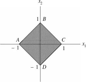
Figure2.1illustrates the geometrical meaning of the open and closed unit spheres.
S1=Parallelogram with vertices(−1,0), (0,1), (1,0), (0,−1).
S1=Parallelogram without sides AB, BC, CD, and DA. Surface or boundary of the closed unit sphere is lines AB, BC, CD, and DA.
(b) If we considerR2with respect to the norm(2)in Example2.2, Fig.2.2 repre-sents the open and closed unit spheres. The rectangle ABCD=S1,where S1 is the rectangle without the four sides.
Fig. 2.1 The geometrical meaning of open and closed unit spheres in Example2.2 (1)
x2
x1 1 B
– 1 D – 1
A
Fig. 2.2 The geometrical meaning of open and closed unit spheres in Example2.2 (2)
x2
x1 1
B
– 1 D
– 1 A
1
C
S1= {x=(x1,x2)∈R2/max(|x1|,|x2|)≤1}
S1= {x=(x1,x2)∈R2/max(|x1|,|x2|) <1}
Surface or boundary S is given by
S = {x=(x1,x2)∈R2/max(|x1|,|x2|)=1}
=Sides AB, BC, CD and DA
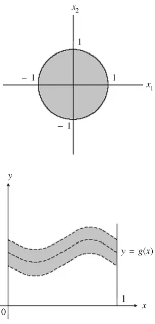
(c) Figure2.3illustrates the geometrical meaning of the open and closed unit spheres inR2with respect to norm(3)of Example2.2.
¯
S1= {x=(x1,x2)∈R2/(x21+x22)1/2≤1}
S1= {x=(x1,x2)∈R2/(x21+x 2 2)
1/2< 1}
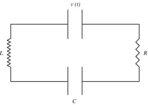
S is the circumference of the circle with center at the origin and radius 1. S1is the interior of the circle with radius 1 and center at the origin.S1¯ is the circle (including the circumference) with center at the origin and radius 1. 3. ConsiderC[0,1]with the norm||f|| = sup
0≤t≤1|
f(t)|. LetS¯r(g)be a closed sphere
inC[0,1]with centergand radiusr. Then,
¯
Sr(g)= {h∈C[0,1]/||g−h|| ≤r}
= {h∈C[0,1]/ sup 0≤x≤1|
g(x)−h(x)| ≤r}
This implies that|g(x)−h(x)| ≤rorh(x)∈ [g(x)−r,g(x)+r]; see Fig.2.4. h(x)lies within the broken lines. One of these is obtained by loweringg(x)by r and other raisingg(x)by the same distance r. It is clear thath(x)∈S⋆
Fig. 2.3 The geometrical meaning of open and closed unit spheres of Example2.2 (3)
x2
x1 1
– 1
– 1 1
Fig. 2.4 The geometrical meaning of open and closed unit spheres inC[0,1]
y
y = g(x)
0
1 x
lies between broken lines and never meets one of them,||h−g||<rand then h(x)∈Sr(g)that ish(x)belongs to k and open ball with center g and radius r. If ||g−h|| =r, then h lies on the boundary of open ballSr(g).
2.4
Bounded and Unbounded Operators
2.4.1
Definitions and Examples
Definition 2.8 LetU andV be two normed spaces. Then,
1. A mappingT fromUintoV is called anoperatoror atransformation. The value ofT atx∈Uis denoted byT(x)orTx.