Volume 108
Intelligent Systems Reference Library
Series Editors
Janusz Kacprzyk
Polish Academy of Sciences, Systems Research Institute, Warsaw, Poland Lakhmi C. Jain
Bournemouth University, University of Canberra and, ACT, Aust Capital Terr, Australia
About this Series
The aim of this series is to publish a Reference Library, including novel advances and
developments in all aspects of Intelligent Systems in an easily accessible and well structured form. The series includes reference works, handbooks, compendia, textbooks, well-structured monographs, dictionaries, and encyclopedias. It contains well integrated knowledge and current information in the field of Intelligent Systems. The series covers the theory, applications, and design methods of
Intelligent Systems. Virtually all disciplines such as engineering, computer science, avionics, business, e-commerce, environment, healthcare, physics and life science are included.
Editors
Roumen Kountchev and Kazumi Nakamatsu
New Approaches in Intelligent Image Analysis
Editors
Roumen Kountchev
Department of Radio Communications and Video Technologies, Technical University of Sofia, Sofia, Bulgaria
Kazumi Nakamatsu
School of Human Science and Environment, University of Hyogo, Himeji, Japan
ISSN 1868-4394 e-ISSN 1868-4408
ISBN 978-3-319-32190-5 e-ISBN 978-3-319-32192-9 DOI 10.1007/978-3-319-32192-9
Library of Congress Control Number: 2016936421 © Springer International Publishing Switzerland 2016
This work is subject to copyright. All rights are reserved by the Publisher, whether the whole or part of the material is concerned, specifically the rights of translation, reprinting, reuse of illustrations, recitation, broadcasting, reproduction on microfilms or in any other physical way, and transmission or information storage and retrieval, electronic adaptation, computer software, or by similar or dissimilar methodology now known or hereafter developed.
The use of general descriptive names, registered names, trademarks, service marks, etc. in this publication does not imply, even in the absence of a specific statement, that such names are exempt from the relevant protective laws and regulations and therefore free for general use.
The publisher, the authors and the editors are safe to assume that the advice and information in this book are believed to be true and accurate at the date of publication. Neither the publisher nor the authors or the editors give a warranty, express or implied, with respect to the material contained herein or for any errors or omissions that may have been made.
Printed on acid-free paper
Preface
This book represents the advances in the development of new approaches, used for the intelligent image analysis. It introduces various aspects of the image analysis, related to the theory for their processing, and to some practical applications.
The book comprises 11 chapters, whose authors are researchers from different countries: USA, Russia, Bulgaria, Japan, Brazil, Romania, Ukraine, and Egypt. Each chapter is a small monograph, which represents the recent research work of the authors in the corresponding scientific area. The object of the investigation is new methods, algorithms, and models, aimed at the intelligent analysis of signals and images—single and sequences of various kinds: natural, medical, multispectral, multi-view, sound pictures, acoustic maps of sources, etc.
New Approaches for Hierarchical Image Decomposition, Based on IDP,
SVD, PCA, and KPCA
In Chap. 1 the basic methods for hierarchical decomposition of grayscale and color images, and of sequences of correlated images are analyzed. New approaches are introduced for hierarchical image decomposition: the Branched Inverse Difference Pyramid (BIDP) and the Hierarchical Singular Value Decomposition (HSVD) with tree-like computational structure for single images; the
Hierarchical Adaptive Principle Component Analysis (HAPCA) for groups of correlated images and the Hierarchical Adaptive Kernel Principal Component Analysis (HAKPCA) for color images. In the chapter the evaluation of the computational complexity of the algorithms used for the implementation of these decompositions is also given. The basic application areas are defined for efficient image hierarchical decomposition, such as visual information redundancy reduction; noise filtration; color segmentation; image retrieval; image fusion; dimensionality reduction, where the following is
executed: the objects classification; search enhancement in large-scale image databases, etc.
Intelligent Digital Signal Processing and Feature Extraction Methods
The goal of Chap. 2 is to present well-known signal processing methods and the way they can be combined with intelligent systems in order to create powerful feature extraction techniques. In order to achieve this, several case studies are presented to illustrate the power of hybrid systems. The main emphasis is on the instantaneous time–frequency analysis, since it is proven to be a powerful method in several technical and scientific areas. The oldest and most utilized method is the Fourier transform, which has been applied in several domains of data processing, but it has very strong limitations due to the constraints it imposes on the analyzed data. Then the short-time Fourier transform and the
wavelet transform are presented as they provide both temporal and frequency information as opposed to the Fourier transform. These methods form the basis of most applications, as they offer the
possibility of time–frequency analysis of signals. The Hilbert–Huang transform is presented as a novel signal processing method, which introduces the concept of the instantaneous frequency that can be determined for every time point, making it possible to have a deeper look into different
signal processing will result in hybrid intelligent systems capable of solving computationally difficult problems.
Multi-dimensional Data Clustering and Visualization via Echo State
Networks
Chapter 3 summarizes the proposed recently approach for multidimensional data clustering and visualization. It uses a special kind of recurrent networks called Echo State Networks (ESN) to generate multiple 2D projections of the multidimensional original data. The 2D projections are
subjected to selection based on different criteria depending on the aim of particular clustering task to be solved. The selected projections are used to cluster and/or to visualize the original data set.
Several examples demonstrate the possible ways to apply the proposed approach to variety of multidimensional data sets: steel alloys discrimination by their composition; Earth cover
classification from hyperspectral satellite images; working regimes classification of an industrial plant using data from multiple measurements; discrimination of patterns of random dot motion on the screen; and clustering and visualization of static and dynamic “sound pictures” by multiple randomly placed microphones.
Unsupervised Clustering of Natural Images in Automatic Image
Annotation Systems
Chapter 4 is devoted to automatic annotation of natural images joining the strengths of the text-based and the content-based image retrieval. The automatic image annotation is based on the semantic concept models, which are built from large number of patches received from a set of images. In this case, image retrieval is implemented by keywords called Visual Words (VWs) that is similar to text document retrieval. The task involves two main stages: a low-level segmentation based on color, texture, and fractal descriptors and a high-level clustering of received descriptors into the separated clusters corresponding to the VWs set. The enhanced region descriptor including color, texture, and fractal features has been proposed. For the VWs generation, the unsupervised clustering is a suitable approach. The Enhanced Self-Organizing Incremental Neural Network (ESOINN) was chosen due to its main benefits as a self-organizing structure and online implementation. The preliminary image segmentation permitted to change a sequential order of descriptors entering the ESOINN as
associated sets. Such approach simplified, accelerated, and decreased the stochastic variations of the ESOINN. The experiments demonstrate acceptable results of the VWs clustering for a non-large natural image sets. This approach shows better precision values and execution time as compared to the fuzzy c-means algorithm and the classic ESOINN. Also issues of parallel implementation of unsupervised segmentation in OpenMP and Intel Cilk Plus environments were considered for processing of HD-quality images.
An Evolutionary Optimization Control System for Remote Sensing
Image Processing
(DPSO)—one novel application of DPSO—coupled with remote sensing image processing to help in the image data analysis. The remote sensing image analysis has been a topic of ongoing research for many years and has led to paradigm shifts in the areas of resource management and global biophysical monitoring. Due to distortions caused by variations in signal/image capture and environmental
changes, there is not a definite model for image processing tasks in remote sensing and such tasks are traditionally approached on a case-by-case basis. Intelligent control, however, can streamline some of the case-by-case scenarios and allows faster, more accurate image processing to support the more accurate remote sensing image analysis.
Tissue Segmentation Methods Using 2D Histogram Matching in a
Sequence of MR Brain Images
In Chap. 6 a new transductive learning method for tissue segmentation using a 2D histogram
modification, applied to Magnetic Resonance (MR) image sequence, is introduced. The 2D histogram is produced from a normalized sum of co-occurrence matrices of each MR image. Two types of
model 2D histograms are constructed for each subsequence: intra-tissue 2D histogram to separate tissue regions and an inter-tissue edge 2D histogram. First, the MR image sequence is divided into few subsequences, using wave hedges distance between the 2D histograms of the consecutive MR images. The test 2D histogram segments are modified in the confidence interval and the most
representative entries for each tissue are extracted, which are used for the kNN classification after distance learning. The modification is applied by using LUT and two ways of distance metric
learning: large margin nearest neighbor and neighborhood component analysis. Finally, segmentation of the test MR image is performed using back projection with majority vote between the probability maps of each tissue region, where the inter-tissue edge entries are added with equal weights to
corresponding tissues. The proposed algorithm has been evaluated with free access data sets and has showed results that are comparable to the state-of-the-art segmentation algorithms, although it does not consider specific shape and ridges of brain tissues.
Multistage Approach for Simple Kidney Cysts Segmentation in CT
Images
Audio Visual Attention Models in Mobile Robots Navigation
In Chap. 8 , it is proposed to use the exiting definitions and models for human audio and visual attention, adapting them to the models of mobile robots audio and visual attention, and combining with the results from mobile robots audio and visual perception in the mobile robots navigation tasks. The mobile robots are equipped with sensitive audio visual sensors (usually microphone arrays and video cameras). They are the main sources of audio and visual information to perform suitable mobile robots navigation tasks modeling human audio and visual perception. The audio and visual perception algorithms are widely used, separately or in audio visual perception, in mobile robot navigation, for example to control mobile robots motion in applications like people and objects
tracking, surveillance systems, etc. The effectiveness and precision of the audio and visual perception methods in mobile robots navigation can be enhanced combining audio and visual perception with audio and visual attention. There exists relative sufficient knowledge describing the phenomena of human audio and visual attention.
Local Adaptive Image Processing
Three methods for 2D local adaptive image processing are presented in Chap. 9 . In the first one, the adaptation is based on the local information from the four neighborhood pixels of the processed image and the interpolation type is changed to zero or bilinear. The analysis of the local
characteristics of images in small areas is presented, from which the optimal selection of thresholds for dividing into homogeneous and contour blocks is made and the interpolation type is changed adaptively. In the second one, the adaptive image halftoning is based on the generalized 2D Last Mean Square (LMS) error-diffusion filter for image quantization. The thresholds for comparing the input image levels are calculated from the gray values dividing the normalized histogram of the input halftone image into equal parts. In the third one, the adaptive line prediction is based on the 2D LMS adaptation of coefficients of the linear prediction filter for image coding. An analysis of properties of 2D LMS filters in different directions was made. The principal block schemes of the developed algorithms are presented. An evaluation of the quality of the processed images was made on the base of the calculated objective criteria and the subjective observation. The given experimental results, from the simulation for each of the developed algorithms, suggest that the effective use of local
information contributes to minimize the processing error. The methods are suitable for different types of images (fingerprints, contour images, cartoons, medical signals, etc.). The developed algorithms have low computational complexity and are suitable for real-time applications.
Machine Learning Techniques for Intelligent Access Control
is physically unique and cannot be duplicated. Biometrics has been used for ages as an access control security system.
Experimental Evaluation of Opportunity to Improve the Resolution of
the Acoustic Maps
Chapter 11 is devoted to generation of acoustic maps. The experimental work considers the possibility to increase the maps resolution. The work uses 2D microphone array with randomly spaced elements to generate acoustic maps of sources located in its near-field region. In this region the wave front is not flat and the phase of the input signals depends on the arrival direction, and on the range as well. The input signals are partially distorted by the indoor multipath propagation and the related interference of sources emissions. For acoustic mapping with improved resolution an algorithm in the frequency domain is proposed. The algorithm is based on the modified method of Capon. Acoustic maps of point-like noise sources are generated. The maps are compared with the maps generated using other famous methods including built-in equipment software. The obtained results are valuable in the estimation of direction of arrival for Noise Exposure Monitoring.
This book will be very useful for students and Ph.D. students, researchers, and software
developers, working in the area of digital analysis and recognition of multidimensional signals and images.
Contents
1 New Approaches for Hierarchical Image Decomposition, Based on IDP, SVD, PCA and KPCA
Roumen Kountchev and Roumiana Kountcheva
1.1 Introduction
1.2 Related Work
1.3 Image Representation Based on Branched Inverse Difference Pyramid
1.3.1 Principles for Building the Inverse Difference Pyramid
1.3.2 Mathematical Representation of n-Level IDP
1.3.3 Reduced Inverse Difference Pyramid
1.3.4 Main Principle for Branched IDP Building
1.3.5 Mathematical Representation for One BIDP Branch
1.3.6 Transformation of the Retained Coefficients into Sub-blocks of Size 2 × 2
1.3.7 Experimental Results
1.4 Hierarchical Singular Value Image Decomposition
1.4.1 SVD Algorithm for Matrix Decomposition
1.4.2 Particular Case of the SVD for Image Block of Size 2 × 2
1.4.3 Hierarchical SVD for a Matrix of Size 2 n × 2 n
1.4.4 Computational Complexity of the Hierarchical SVD of Size 2 n × 2 n 1.4.5 Representation of the HSVD Algorithm Through Tree-like Structure
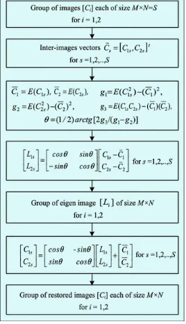
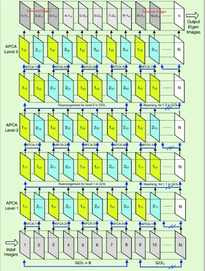
1.5 Hierarchical Adaptive Principal Component Analysis for Image Sequences
1.5.1 Principle for Decorrelation of Image Sequences by Hierarchical Adaptive PCA
1.5.2 Description of the Hierarchical Adaptive PCA Algorithm
1.5.4 Experimental Results
1.6 Hierarchical Adaptive Kernel Principal Component Analysis for Color Image Segmentation
1.6.1 Mathematical Representation of the Color Adaptive Kernel PCA
1.6.2 Algorithm for Color Image Segmentation by Using HAKPCA
1.6.3 Experimental Results
1.7 Conclusions
2 Intelligent Digital Signal Processing and Feature Extraction Methods
János Szalai and Ferenc Emil Mózes
2.1 Introduction
2.2 The Fourier Transform
2.2.1 Application of the Fourier Transform
2.3 The Short-Time Fourier Transform
2.3.1 Application of the Short-Time Fourier Transform
2.4 The Wavelet Transform
2.4.1 Application of the Wavelet Transform
2.5 The Hilbert-Huang Transform
2.5.1 Introducing the Instantaneous Frequency
2.5.2 Computing the Instantaneous Frequency
2.5.3 Application of the Hilbert-Huang Transform
2.6 Hybrid Signal Processing Systems
2.6.1 The Discrete Wavelet Transform and Fuzzy C-Means Clustering
2.6.2 Automatic Sleep Stage Classification
2.6.3 The Hilbert-Huang Transform and Support Vector Machines
References
3 Multi-dimensional Data Clustering and Visualization via Echo State Networks
Petia Koprinkova-Hristova
3.1 Introduction
3.2 Echo State Networks and Clustering Procedure
3.2.1 Echo State Networks Basics
3.2.2 Effects of IP Tuning Procedure
3.2.3 Clustering Algorithms
3.3 Examples
3.3.1 Clustering of Steel Alloys in Dependence on Their Composition
3.3.2 Clustering and Visualization of Multi-spectral Satellite Images
3.3.3 Clustering of Working Regimes of an Industrial Plant
3.3.4 Clustering of Time Series from Random Dots Motion Patterns
3.3.5 Clustering and 2D Visualization of “Sound Pictures”
3.4 Summary of Results and Discussion
3.5 Conclusions
References
4 Unsupervised Clustering of Natural Images in Automatic Image Annotation Systems
Margarita Favorskaya, Lakhmi C. Jain and Alexander Proskurin
4.1 Introduction
4.2 Related Work
4.2.1 Unsupervised Segmentation of Natural Images
4.2.2 Unsupervised Clustering of Images
4.3 Preliminary Unsupervised Image Segmentation
4.4.1 Color Features Representation
4.4.2 Calculation of Texture Features
4.4.3 Fractal Features Extraction
4.4.4 Enhanced Region Descriptor
4.4.5 Parallel Computations of Features
4.5 Clustering of Visual Words by Enhanced SOINN
4.5.1 Basic Concepts of ESOINN
4.5.2 Algorithm of ESOINN Functioning
4.6 Experimental Results
4.7 Conclusion and Future Development
References
5 An Evolutionary Optimization Control System for Remote Sensing Image Processing
Victoria Fox and Mariofanna Milanova
5.1 Introduction
5.2 Background Techniques
5.2.1 Darwinian Particle Swarm Optimization
5.2.2 Total Variation for Texture-Structure Separation
5.2.3 Multi-phase Chan-Vese Active Contour Without Edges
5.3 Evolutionary Optimization of Segmentation
5.3.1 Darwinian PSO for Thresholding
5.3.2 Novel Darwinian PSO for Relative Total Variation
5.3.3 Multi-phase Active Contour Without Edges with Optimized Initial Level Mask
5.3.4 Workflow of Proposed System
5.4.1 Results
5.4.2 Discussion
5.4.3 Conclusion and Future Research
References
6 Tissue Segmentation Methods Using 2D Histogram Matching in a Sequence of MR Brain Images
Vladimir Kanchev and Roumen Kountchev
6.1 Introduction
6.2 Related Works
6.3 Overview of the Developed Segmentation Algorithm
6.4 Preprocessing and Construction of a Model and Test 2D Histograms
6.4.1 Transductive Learning
6.4.2 MRI Data Preprocessing
6.4.3 Construction of a 2D Histogram
6.4.4 Separation into MR Image Subsequences
6.4.5 Types of 2D Histograms and Preprocessing
6.5 Matching and Classification of a 2D Histogram
6.5.1 Construct Train 2D Histogram Segments Using 2D Histogram Matching
6.5.2 2D Histogram Classification After Distance Metric Learning
6.6 Segmentation Through Back Projection
6.7 Experimental Results
6.7.1 Test Data Sets and Parameters of the Developed Algorithm
6.7.2 Segmentation Results
6.8 Discussion
References
7 Multistage Approach for Simple Kidney Cysts Segmentation in CT Images
Veska Georgieva and Ivo Draganov
7.1 Introduction
7.1.1 Medical Aspect of the Problem for Kidney Cyst Detection
7.1.2 Review of Segmentation Methods
7.1.3 Proposed Approach
7.2 Preprocessing Stage of CT Images
7.2.1 Noise Reduction with Median Filter
7.2.2 Noise Reduction Based on Wavelet Packet Decomposition and Adaptive Threshold
7.2.3 Contrast Limited Adaptive Histogram Equalization (CLAHE)
7.3 Segmentation Stage
7.3.1 Segmentation Based on Split and Merge Algorithm
7.3.2 Clustering Classification of Segmented CT Image
7.3.3 Segmentation Based on Texture Analysis
7.4 Experimental Results
7.5 Discussion
7.6 Conclusion
References
8 Audio Visual Attention Models in the Mobile Robots Navigation
Snejana Pleshkova and Alexander Bekiarski
8.1 Introduction
8.2 Related Work
8.3 The Basic Definitions of the Human Audio Visual Attention
8.5 Audio Visual Attention Model Applied in the Audio Visual Mobile Robot System
8.5.1 Room Environment Model for Description of Indoor Initial Audio Visual Attention
8.5.2 Development of the Algorithm for Definition of the Mobile Robot Initial Audio Visual Attention Model
8.5.3 Definition of the Initial Mobile Robot Video Attention Model with Additional Information from the Laser Range Finder Scan
8.5.4 Development of the Initial Mobile Robot Video Attention Model Localization with Additional Information from a Speaker to the Mobile Robot Initial Position
8.6 Definition of the Probabilistic Audio Visual Attention Mobile Robot Model in the Steps of the Mobile Robot Navigation Algorithm
8.7 Experimental Results from the Simulations of the Mobile Robot Motion Navigation Algorithm Applying the Probabilistic Audio Visual Attention Model
8.7.1 Experimental Results from the Simulations of the Mobile Robot Motion Navigation Algorithm Applying Visual Perception Only
8.7.2 Experimental Results from the Simulations of the Mobile Robot Motion Navigation Algorithm Using Visual Attention in Combination with the Visual Perception
8.7.3 Quantitative Comparison of the Simulations Results Applying Visual Perception Only, and Visual Attention with Visual Perception
8.7.4 Experimental Results from Simulations Using Audio Visual Attention in Combination with Audio Visual Perception
8.7.5 Quantitative Comparison of the Results Achieved in Simulations Applying Audio Visual Perception Only, and Visual Attention Combined with Visual Perception
8.8 Conclusion
References
9 Local Adaptive Image Processing
Rumen Mironov
9.1 Introduction
9.2 Method for Local Adaptive Image Interpolation
9.2.2 Analysis of the Characteristics of the Filter for Two-Dimensional Adaptive Interpolation
9.2.3 Evaluation of the Error of the Adaptive 2D Interpolation
9.2.4 Functional Scheme of the 2D Adaptive Interpolator
9.3 Method for Adaptive 2D Error Diffusion Halftoning
9.3.1 Mathematical Description of Adaptive 2D Error-Diffusion
9.3.2 Determining the Weighting Coefficients of the 2D Adaptive Halftoning Filter
9.3.3 Functional Scheme of 2D Adaptive Halftoning Filter
9.3.4 Analysis of the Characteristics of the 2D Adaptive Halftoning Filter
9.4 Method for Adaptive 2D Line Prediction of Halftone Images
9.4.1 Mathematical Description of Adaptive 2D Line Prediction
9.4.2 Synthesis and Analysis of Adaptive 2D LMS Codec for Linear Prediction
9.5 Experimental Results
9.5.1 Experimental Results from the Work of the Developed Adaptive 2D Interpolator
9.5.2 Experimental Results from the Work of the Developed Adaptive 2D Halftoning Filter
9.5.3 Experimental Results from the Work of the Developed Codec for Adaptive 2D Linear Prediction
9.6 Conclusion
References
10 Machine Learning Techniques for Intelligent Access Control
Wael H. Khalifa, Mohamed I. Roushdy and Abdel-Badeeh M. Salem
10.1 Introduction
10.2 Machine Learning Methodology for Biometrics
10.2.1 Signal Capturing
10.2.3 Classification
10.3 User Authentication Techniques
10.4 Physiological Biometrics Taxonomy
10.4.1 Finger Print
10.4.2 Face
10.4.3 Iris
10.5 Behavioral Biometrics Taxonomy
10.5.1 Keystroke Dynamics
10.5.2 Voice
10.5.3 EEG
10.6 Multimodal Biometrics
10.7 Applications
10.8 Machine Learning Techniques for Biometrics
10.8.1 Fisher’s Discriminant Analysis
10.8.2 Linear Discriminant Classifier
10.8.3 LVQ Neural Net
10.8.4 Neural Networks
10.9 Conclusion
References
11 Experimental Evaluation of Opportunity to Improve the Resolution of the Acoustic Maps
Volodymyr Kudriashov
11.1 Introduction
11.2 Theoretical Part
11.2.2 Signal Model
11.2.3 Acoustic Mapping Methods
11.3 The Experimental Acoustic Camera Equipment
11.4 Experimental Results
11.4.1 Microphone Array Patterns Generated with the Delay-and-Sum Beamforming Method
11.4.2 Microphone Array Patterns Generated with the Christensen Beamforming Method
11.4.3 Microphone Array Patterns Generated with the Modified Capon-Based Beamforming Method
11.4.4 Microphone Array Responses for Two Point-like Emitters
11.4.5 The Acoustic Camera Responses for Two Point-like Emitters
11.5 Conclusions
Contributors
Alexander BekiarskiDepartment of Telecommunications, Technical University of Sofia, Sofia, Bulgaria
Ivo Draganov
Department of Radio Communications and Video Technologies, Technical University of Sofia, Sofia, Bulgaria
Margarita Favorskaya
Institute of Informatics and Telecommunications, Siberian State Aerospace University, Krasnoyarsk, Russian Federation
Victoria Fox
Department of Mathematics, University of Arkansas at Monticello, Monticello, Arkansas, USA
Veska Georgieva
Department of Radio Communications and Video Technologies, Technical University of Sofia, Sofia, Bulgaria
Lakhmi C. Jain
Bournemouth University, Fern Barrow, Poole, UK University of Canberra, Canberra, Australia
Vladimir Kanchev
Department of Radio Communications and Video Technologies, Technical University of Sofia, Sofia, Bulgaria
Wael H. Khalifa
Artificial Intelligence and Knowledge Engineering Research Labs, Computer Science Department, Faculty of Computer and Information sciences, Ain Shams University, Cairo, Egypt
Petia Koprinkova-Hristova
Bulgarian Academy of Sciences, Institute of Information and Communication Technologies, Sofia, Bulgaria
Roumen Kountchev
Department of Radio Communications and Video Technologies, Technical University of Sofia, Sofia, Bulgaria
Roumiana Kountcheva
T&K Engineering Co., Sofia, Bulgaria
Mathematical Methods for Sensor Information Processing Department, Institute of Information and Communication Technologies, Bulgarian Academy of Sciences, Sofia, Bulgaria
Mariofanna Milanova
Computer Science Department, University of Arkansas at Little Rock, Little Rock, Arkansas, USA
Ferenc Emil Mózes
Petru Maior University of Târgu Mures, Târgu Mures, Romania
Rumen Mironov
Department of Radio Communications and Video Technologies, Technical University of Sofia, Sofia, Bulgaria
Snejana Pleshkova
Department of Telecommunications, Technical University of Sofia, Sofia, Bulgaria
Alexander Proskurin
Institute of Informatics and Telecommunications, Siberian State Aerospace University, Krasnoyarsk, Russian Federation
Mohamed I. Roushdy
Artificial Intelligence and Knowledge Engineering Research Labs, Computer Science Department, Faculty of Computer and Information sciences, Ain Shams University, Cairo, Egypt
Abdel-Badeeh M. Salem
Artificial Intelligence and Knowledge Engineering Research Labs, Computer Science Department, Faculty of Computer and Information sciences, Ain Shams University, Cairo, Egypt
János Szalai
(1)
(2)
© Springer International Publishing Switzerland 2016
Roumen Kountchev and Kazumi Nakamatsu (eds.), New Approaches in Intelligent Image Analysis, Intelligent Systems Reference Library 108, DOI 10.1007/978-3-319-32192-9_1
1. New Approaches for Hierarchical Image
Decomposition, Based on IDP, SVD, PCA and KPCA
Roumen Kountchev
1and Roumiana Kountcheva
2Department of Radio Communications and Video Technologies, Technical University of Sofia, 8 Kl. Ohridski Blvd., 1000 Sofia, Bulgaria
T&K Engineering Co., Drujba 2, Bl. 404/2, 1582 Sofia, Bulgaria
Roumen Kountchev (Corresponding author) Email: [email protected]
Roumiana Kountcheva
Email: [email protected]
Abstract
The contemporary forms of image representation vary depending on the application. There are well-known mathematical methods for image representation, which comprise: matrices, vectors,
determined orthogonal transforms, multi-resolution pyramids, Principal Component Analysis (PCA) and Independent Component Analysis (ICA), Singular Value Decomposition (SVD), wavelet sub-band decompositions, hierarchical tensor transformations, nonlinear decompositions through hierarchical neural networks, polynomial and multiscale hierarchical decompositions,
multidimensional tree-like structures, multi-layer perceptual and cognitive models, statistical models, etc. In this chapter are analyzed the basic methods for hierarchical decomposition of grayscale and color images, and of sequences of correlated images of the kind: medical, multispectral, multi-view, etc. Here is also added one expansion and generalization of the ideas of the authors from their
previous publications, regarding the possibilities for the development of new, efficient algorithms for hierarchical image decompositions with various purposes. In this chapter are presented and analyzed the following four new approaches for hierarchical image decomposition: the Branched Inverse Difference Pyramid (BIDP), based on the Inverse Difference Pyramid (IDP); the Hierarchical Singular Value Decomposition (HSVD) with tree-like computational structure; the Hierarchical Adaptive Principle Component Analysis (HAPCA) for groups of correlated images; and the
decomposition of multidimensional images are specified. On the basis of the results obtained from the executed analysis, the basic application areas for efficient image processing are specified, such as: reduction of the information surplus; noise filtration; color segmentation; image retrieval; image fusion; dimensionality reduction for objects classification; search enhancement in large scale image databases, etc.
Keywords Hierarchical image decomposition – Branched inverse difference pyramid – Hierarchical singular value decomposition – Hierarchical principal component analysis for groups of images – Hierarchical adaptive kernel principal component analysis for color images
1.1 Introduction
The methods for image processing, transmission, registration, restoration, analysis and recognition, are defined at high degree by the corresponding mathematical forms and models for their
representation. On the other hand, they all depend on the way the image was created, and on their practical use. The primary forms for image representation depend on the used sources, such as: photo and video cameras, scanners, ultrasound sensors, X-ray, computer tomography, etc. The matrix
descriptions are related to the primary discrete forms. Each still halftone image is represented by one matrix; the color RGB image—by three matrices; the multispectral, hyper spectral and multi-view images, and also some kinds of medical images (for example, computer tomography, IMR, etc.)—by
N matrices (for N > 3), while the moving images are represented through M temporal sequences, of N
matrices each. There are already many secondary forms created for image representation, obtained from the primary forms, after reduction of the information surplus, and depending on the application. Various mathematical methods are used to transform the image matrices into reduced (secondary) forms by using: vectors, for each image block, through which are composed vector fields;
deterministic and statistical orthogonal transforms; multi-resolution pyramids; wavelet sub-band decompositions; hierarchical tensor transforms; nonlinear decompositions through hierarchical neural networks, polynomial and multiscale hierarchical decompositions, multi-dimensional tree-like
structures, multi-layer perceptual and cognitive models, statistical models, fuzzy hybrid methods for image decomposition, etc.
The decomposition methods permit each image matrix to be represented as the sum of the matrix components with different weights, defined by the image contents. Besides, the description of each matrix in the decomposition is much simpler than that of the original (primary) matrix. The number of the matrices in the decomposition could be significantly reduced through analyzing their weights, without significant influence on the approximation accuracy of the primary matrix. To this group could be related the methods for linear orthogonal transforms [1]: the Discrete Fourier Transform (DFT), the Discrete Cosine Transform (DCT), the Walsh-Hadamard Transform (WHT), the Hartley Transform (HrT), the Haar Transform (HT), etc.; the pyramidal decompositions [2]: the Gaussian Pyramid (GP), the Laplacean Pyramid (LP), the Discrete Wavelet Transform (DWT), the Discrete Curvelet Transform (DCuT) [3], the Inverse Difference Pyramid (IDP) [4], etc.; the statistical
decompositions [5]: the Principal Component Analysis (PCA), the Independent Component Analysis (ICA) and the Singular Value Decomposition (SVD); the polynomial and multiscale hierarchical decompositions [6, 7]; multi-dimensional tree-like structures [8]; hierarchical tensor transformations [9]; the decompositions based on hierarchical neural networks [10]; etc.
decomposition. Here are also generalized the following new approaches for hierarchical
decomposition of multi-component matrix images: the Branched Inverse Difference Pyramid (BIDP), based on the Inverse Difference Pyramid (IDP), the Hierarchical Singular Value Decomposition (HSVD)—for the representation of single images; the Hierarchical Adaptive Principal Component Analysis (HAPCA)—for the decorrelation of sequences of images, and the Hierarchical Adaptive Kernel Principal Component Analysis (HAKPCA)—for the analysis of color images.
1.2 Related Work
One of the contemporary methods for hierarchical image decomposition is called multiscale
decomposition [7]. It is used for noise filtration in the image f, represented by the sum of the clean part u, and the noisy part, v. In accordance to Rudin, Osher and Fatemi (ROF) [11], to define the components u and v it is necessary to calculate the total variation of the functional Q, defined by the relation:
where λ > 0 is a scale parameter; and f ∈ L2(Ω)—the image function, defined in the space L2(Ω).
The minimization of Q leads to decomposition, in result of which the visual information is divided into a part u that extracts the edges of f, and a part v that captures the texture. Denoising at different scales λ generates a multiscale image representation. In [6], Tadmor, Nezzar and Vese proposed a multiscale image decomposition which offers a hierarchical and adaptive representation for different features in the analyzed images. The image is hierarchically decomposed into the sum of simpler atoms u k , where u k extracts more refined information from the previous scale uk−1. To this end, the atoms u k are obtained as dyadically scaled minimizers of the ROF functionals at increasing λ k
scales. Thus, starting with v−1 := f and letting v k denote the residual at a given dyadic scale, λ k = 2k , the recursive step [uk , vk ] = arg{inf[Q T(v k−1, k)]} leads to the desired hierarchical
decomposition, f = ΣT(u k ) (here T is a blurring operator).
Another well-known approach for hierarchical decomposition is based on the hierarchical matrices [12]. The concept of hierarchical, or H-matrices, is based on the observation that submatrices of a full rank matrix may be of low rank, and respectively—to have low rank approximations. On Fig. 1.1 is given an example for the representation of a matrix of size 8 × 8 through H-matrices, which contain sub-matrices of three different sizes: 4 × 4, 2 × 2 and 1 × 1.
Fig. 1.1 Representation of the matrix of size 8 × 8 through three hierarchical matrices, or H-matrices
matrices have, under certain assumptions, submatrices with exponentially decaying singular values. This means that these submatrices have also good low rank approximations. The hierarchical
matrices permit decomposition by QR or Cholesky algorithms, which are iterative. Unlike them, the new approaches for hierarchical image decomposition, given in this chapter (BIDP and HSVD—for single images, HAPCA—for groups of correlated images, and HAKPCA—for color images), are not based on iterative algorithms.
1.3 Image Representation Based on Branched Inverse Difference
Pyramid
1.3.1 Principles for Building the Inverse Difference Pyramid
In this section is given a short description of the inverse difference pyramid, IDP [4, 13], used as a basis for building its modifications. Unlike the famous Gaussian (GP) and Laplacian (LP) pyramids, the IDP represents the image in the spectral domain. After the decomposition, the image energy is concentrated in its first components, which permits to achieve very efficient compression, by cutting off the low-energy components. As a result, the main part of the energy of the original image is
retained, despite the limited number of decomposition components used. For the decomposition implementation various kinds of orthogonal transforms could be used. In order to reduce the number of decomposition levels and the computational complexity, the image is initially divided into blocks and for each is then built the corresponding IDP.
In brief, the IDP is executed as follows: At the lowest (initial) level, on the matrix [B] of size 2n × 2nis applied the pre-selected “Truncated” Orthogonal Transform (TOT) and are calculated the values of a relatively small number of “retained” coefficients, located in the high-energy area of the so calculated transformed (spectrum) matrix [S 0 ]. These are usually the coefficients with spatial frequencies (0, 0), (0, 1), (1, 0) and (1, 1). After Inverse Orthogonal Transform (IOT) of the
“truncated” spectrum matrix , which contains the retained coefficients only, is obtained the matrix for the initial IDP level (p = 0), which approximates the matrix [B]. The accuracy of the
approximation depends on: the positions of the retained coefficients in the matrix [S 0]; the values, used to substitute the missing coefficients from the approximating matrix for the zero level, and on the selected orthogonal transform. In the next decomposition level (p = 1), is calculated the difference matrix . The resulting matrix is then split into 4 sub-matrices of size 2 n−1 ×2n−1 and on each is applied the corresponding TOT. The total number of retained coefficients
TOT, etc. In the last (highest) IDP level is obtained the “residual” difference matrix. In case that the image should be losslessly coded, each block of the residual matrix is processed with full orthogonal transform and no coefficients are omitted.
1.3.2 Mathematical Representation of n-Level IDP
The digital image is represented by a matrix of size (2n m) × (2nm). For the processing, the matrix is first divided into blocks of size 2n × 2nand on each is applied the IDP decomposition. The matrix [B(2n )] of each block is represented by the equation:
(1.1) Here the number of decomposition components, which are matrices of size 2n × 2n, is equal to
(r + 2). The maximum possible number of decomposition levels for one block is n + 1 (for r = n − 1). The last component defines the approximation error for the block for the case, when the decomposition is limited up to level p = r. The first component for the level p = 0 is the coarse approximation of the block [B(2n)]. It is obtained through 2D IOT on the block in correspondence with the relation:
(1.2) where is a matrix of size 2n × 2n, used for the inverse orthogonal transform of
.
The matrix is the “truncated” orthogonal transform of the block [B(2n)].
Here m0(u, v) are the elements of the binary matrix-mask [M 0(2n)], used to define the retained
coefficients of in correspondence to the relation:
(1.3) The values of the elements are selected in accordance with the requirement the retained coefficients to be these with maximum energy, calculated for all image blocks. The transform of the block [B(2n)] is defined through direct 2D OT:
(1.4) where is a matrix of size 2n × 2nfor the decomposition level p = 0, used to perform the selected 2D OT, which could be DFT, DCT, WHT, KLT, etc.
The remaining coefficients in the decomposition presented by Eq. 1.1 are the approximating difference matrices for levels p = 1, 2, …, r. They comprise the sub-matrices
of size 2n−p × 2n−p for k
(1.5) where 4pis the number of the quadtree branches in the decomposition level p. Here is a matrix of size 2n−p × 2n−pin the level p, used for the inverse 2D OT.
The elements of the matrix are defined by the elements mp (u, v) of the binary matrix-mask [M p(2 n−p)]:
(1.6) The matrix is the transform of and is defined through direct 2D OT:
(1.7) Here is a matrix of size 2n−p × 2n−p in the decomposition level p, used for the 2D OT of each block (when kp = 1, 2,…, 4p ), of the difference matrix for same level, defined by the equation:
(1.8) (1.9) In result of the decomposition represented by Eq. 1.1, for each block [B(2n)], are calculated the
following spectrum coefficients:
all nonzero coefficients of the transform in the decomposition level p = 0;
all nonzero coefficients of the transforms for k p = 1, 2, …, 4pin the decomposition levels p = 1, 2, …, r.
The spectrum coefficients of same spatial frequency (u, v) from all image blocks are arranged in common data sequences, which correspond to their decomposition level p. The transformation of the 2D data massifs into one-dimensional data sequence is executed, using the recursive Hilbert scan, which preserves very well the correlation between neighboring coefficients.
In order to reduce the decomposition complexity, and in accordance with Eq. 1.1, this could be done recursively, as follows:
(1.10) For the case, when the number of the retained coefficients for each IDP sub-block k pof size
is then their total number for all levels is:
1.3.3 Reduced Inverse Difference Pyramid
For the building of the Reduced IDP (RIDP) [14], the existing relations between the spectrum coefficients from the neighboring IDP levels are used. Let the retained coefficients with
spatial frequencies (0, 0), (1, 0), (0, 1) and (1, 1) for the sub-block kp in the IDP level p, be obtained by using the 2D-WHT. Then, except for level p = 0, the coefficients (0, 0) from each of the four
neighboring sub-blocks in same IDP level are equal to zero, i.e.:
(1.12) From this, it follows that the coefficients for i = 0, 1, 2, 3 could be cut-off, and as a
result they should not be saved or transferred. Hence, the total number of the retained coefficients NR
for each sub-block k p in the decomposition levels p = 1, 2,…, n−1 of the RIDP could be reduced by ¼, i.e.
(1.13) In this case the total number of the “retained” coefficients for all levels is equal to the number of pixels in the block, and hence, the so calculated RIPD is “complete”.
1.3.4 Main Principle for Branched IDP Building
The pyramid BIDP [15, 16] with one or more branches is an extension of the basic IDP. The image representation through the BIDP aims at the enhancement of the image energy concentration in a small number of IDP components. On Fig. 1.2 is shown an example block diagram of the generalized 3-level BIDP. The IDP for each block of size 2n × 2n from the original image, called “Main Pyramid”, is of 3 levels (n = 3, for p = 0, 1, 2). The values of the coefficients, calculated for these 3 levels, compose the inverse pyramid, whose sections are of different color each. The coefficients s(0, 0),
s(0, 1), s(1, 0) and s(1, 1) in level p = 0 from all blocks compose corresponding matrices of size
m × m, colored in yellow. These 4 matrices build the “Branch for level 0” of the Main Pyramids. Each is then divided into blocks of size 2n−1 ×2n−1, on which in similar way are built the
Fig. 1.2 Example of generalized 3-level Branched Inverse Difference Pyramid (BIDP)
Each matrix of size 2m × 2m is divided into blocks of size 2n−1 × 2n−1, on which in similar way
are build corresponding 3-level IDPs (p = 10, 11, 12). The retained coefficients, calculated after TOT from the blocks of the Residual Difference in the last level (p = 2) of the Main Pyramids, build matrices of size 4m × 4m; from the first level (p = 00) of the Pyramid Branch 0—matrices of size (m/2n−1 × m/2n−1); and from the first level (p = 10) of the “Pyramid Branch 1”—matrices of size
(m/2n−2 × m/2n−2). In order to reduce the correlation between the elements of the so obtained
matrices, on each group of 4 spatially neighboring elements is applied the following transform: the first is substituted by their average value, and each of the remaining 3—by its difference to next elements, scanned counter-clockwise. The coefficients, obtained this way from all levels of the Main and Branch Pyramids are arranged in one-dimensional sequences in accordance with Hilbert scan and after that are quantizated and entropy coded using Adaptive RLC and Huffman. The values of the spectrum coefficients are quantizated only in case that the image coding is lossy. In order to retain the visual quality of the restored images, the quantization values are related to the sensibility of the
human vision to errors in different spatial frequencies. To reduce these errors, retaining the compression efficiency, in the consecutive BIDP levels could be used various fast orthogonal transforms: for example, in the zero level could be used DCT, and in the next levels—WHT.
1.3.5 Mathematical Representation for One BIDP Branch
In the general case, the branch g of the BIDP is built on the matrix of size
which comprises all spectrum coefficients with the same spatial frequency (u, v) from all blocks or sub-blocks kp in the level p = g of the Main IDPs. By analogy with Eq. (1.1), the matrix
could be decomposed in accordance with the relation, given below:
(1.15) (1.16)
(1.17)
(1.18) (1.19) (1.20) (1.21) All matrices in Eqs. (1.14)−(1.19) are of size and these in Eqs. (1.20) and (1.21) —of size The decomposition from Eq. (1.14) of the matrix is named
Pyramid Branch (PBg(u,v)). It is a pyramid, whose initial and final levels are g and r correspondingly (g < r). This pyramid represents the branch g of the Main IDPs and contains all coefficients, whose spatial frequency is (u, v).
The maximum number of branches for the levels p = 0, 1, …, n − 1 of the Main IDPs, built on a sub-block of size is defined by the general number of retained spectrum coefficients
. For the branch g from the level p = g the corresponding pyramid PBg(uv) is of
r levels. The number of the coefficients in this branch of the Main IDPs for p = g, g + 1, …, r, without cutting-off the coefficients, calculated for the spatial frequency (0, 0), is:
(1.22) In case that the number of the retained spectrum coefficients for each sub-block is set to be
then . In this case, from Eq. (1.22) it follows, that the total number of the
coefficients in the branch PBg(uv) is Hence, the compression ratio (CR) for PBg(uv) is defined by the relation:
(1.23) where 4n−g−1 is the number of the elements in one sub-block of size from PB
g(uv).
The compression ratio for the Main IDPs, calculated in accordance with Eq. (1.11), is:
(1.24) From the comparison of the Eqs. (1.23) and (1.24) it follows, that:
basic pyramids. From Eq. (1.25) it follows that the condition r > 1 is satisfied, when n > 4, i.e., when the image is divided into blocks of minimum size of 16 × 16 pixels. For this case, to retain the
correlation between their pixels high, is necessary the size of the image (16m) × (16m) to be
relatively large. For example, the image should be of size 2k × 2k (for m = 128), or larger. Hence, the BIDP decomposition is efficient mainly for images with high resolution.
The correlation between the elements of the blocks of size from the initial level g = 0 of the Main IDPs is higher than that, between the elements of the sub-blocks of size
from the higher levels g = 1, 2, …, r. Because of this, the branching of the BIDP should always start from the level g = 0.
1.3.6 Transformation of the Retained Coefficients into Sub-blocks of
Size 2 × 2
The aim of the transformation is to reduce the correlation between the retained neighboring spectrum coefficients in the sub-blocks of size 2 × 2 in each matrix, built by the coefficients of same spatial frequency (u, v) from all blocks (or respectively—from the sub-blocks k p in the selected level p of the Main IDPs, or their branches). In order to simplify the presentation, the spectrum coefficients in the sub-blocks k p for the level p, are set as follows:
Fig. 1.3 Location of the retained groups of four spectrum coefficients from 4 neighboring sub-blocks k p + i (i = 0, 1, 2, 3) of size 2
n−p × 2 n−p in the decomposition level p
In correspondence with the symbols, used in Fig. 1.3, the transformation of the groups of four coefficients is represented by the relation below [16]:
(1.27)
Here Pi, for i = 1, 2, 3, 4 represent correspondingly:
the coefficients Ai, for i = 1, 2, 3, 4 with frequencies (0, 0); the coefficients Bi, for i = 1, 2, 3, 4 with frequencies (1, 0); the coefficients Ci, for i = 1, 2, 3, 4 with frequencies (0, 1); the coefficients Di, for i = 1, 2, 3, 4 with frequencies (1, 1).
In result of the transform, executed in accordance with Eq. (1.27), each coefficient S1 has higher value, than the remaining three difference coefficients S 2, S 3, and S 4.
The inverse transform executed in respect of Eq. (1.27) gives total restoration of the initial coefficients Pi, for i = 1, 2, 3, 4:
(1.28)
Depending on the frequency (0, 0), (1, 0), (0, 1), or (1, 1) of the restored coefficients P1 ~ P4, they correspond to A1 ~ A4, B 1 ~ B 4, C1 ~ C 4, or D1 ~ D 4. The operation, given in Eq. (1.28) is executed through decoding of the transformed coefficients S 1 ~ S 4. The so described features of the coefficients S1, S2, S3, S4 permit to achieve significant enhancement of their entropy coding
efficiency.
The basic quality of the BIDP is that it offers significant decorrelation of the processed image data. As a result, the BIDP permits the following:
To achieve highly efficient compression with retained visual quality of the restored image (i.e. visually lossless coding), or efficient lossless coding, depending on the application
requirements;
Layered coding and transfer of the image data, in result of which is obtained low transfer bit-rate with gradually increased quality of the decoded image;
Lower computational complexity than that of the wavelet decompositions [4];
Easy adaptation of the coder parameters, so that to ensure the needed concordance of the obtained data stream, to the ability of the communication channel;
1.
Retaining the quality of the decoded image after multiple coding/decoding;
The BIDP could be further developed and modified in accordance to the requirements of various possible applications. One of these applications for processing of groups of similar images, for example, is a sequence of Computer Tomography (CT) images, Multi-Spectral (MS) images, etc.
1.3.7 Experimental Results
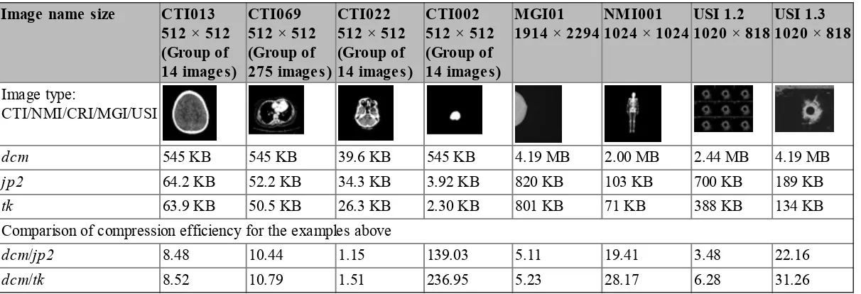
The experimental results, given below, were obtained from the investigation of image database,
which contained medical images stored in DICOM (dcm) format, of various size and kind, grouped in 24 classes. The database was created at the Medical University of Sofia, and comprises the following image kinds: CTI—computer tomography images; MGI—mammography images; NMI—nuclear
magnetic resonance images; CRI—computer radiography images, and USI—ultrasound images. For the investigation, the DICOM images were first transformed into non-compressed (bmp format), and then they were processed by using various lossless compression algorithms. A part of the obtained results is given in Table 1.1.
Table 1.1 Results for the lossless compression of various classes of medical images
Image name size CTI013
Comparison of compression efficiency for the examples above
dcm/jp2 8.48 10.44 1.15 139.03 5.11 19.41 3.48 22.16
dcm/tk 8.52 10.79 1.51 236.95 5.23 28.17 6.28 31.26
Here are shown the results for the lossless compression of the bmp files of still images, and of image sequences, after their transformation into files of the kind jp2 and tk. The image file format jp2 is based on the standard JPEG2000LS, and the tk format—on the algorithms BIDP for single images, combined with the adaptive run-length lossless coding (ARLE), based on the histogram statistics [17]. For the execution of the 2D-TOT/IOT in the initial levels of all basic pyramids and their branches was used the 2D-DCT, and in their higher levels—the 2D-WHT transform. The number of the pyramid levels for the blocks of the smallest treated images (of size 512 × 512), is two, and for the larger ones, it is three. The basic IDP pyramids have one branch only, comprising coefficients with spatial frequency (0, 0) for their initial levels.
From the analysis of the obtained results, the following conclusions could be done:
2.
3.
Together with the enlargement of the analyzed images, the compression ratio for the lossless tk
compression grows up, compared to that of the jp2;
The data given in Table 1.1 show that the mean compression ratio for all DICOM images after their transformation into the format tk is 41:1, while for the jp2 this coefficient is 26:1. Hence, the use of the tk format for all 24 classes ensures compression ratio which is ≈40 % higher than that of the jp2 format.
The experimental results, obtained for the comparison of the coding efficiency for several kinds of medical images through BIDP and JPEG2000 confirmed the basic advantages of the new approach for hierarchical pyramid decomposition, presented here.
1.4 Hierarchical Singular Value Image Decomposition
The SVD is a statistical decomposition for processing, coding and analysis of images, widely used in the computer vision systems. This decomposition was an object of vast research, presented in many monographs [18–22] and papers [23–26]. This is optimal image decomposition, because it
concentrates significant part of the image energy in minimum number of components, and the restored image (after reduction of the low-energy components), has minimum mean square error. One of the basic problems, which limit, to some degree, the use of the “classic” SVD, is related to its high computational complexity, which grows up together with the image size.
To overcome this problem, several new approaches are already offered. The first is based on the SVD calculation through iterative methods, which do not require defining the characteristic
polynomials of a pair of matrices. In this case, the SVD is executed in two stages: in the first, each matrix is first transformed into triangular form with the QR decomposition, and then—into bidiagonal, through the Householder transforms [27]. In the second stage on the bidiagonal matrix is applied an iterative method, whose iterations stop when the needed accuracy is achieved. For this could be used the iterative method of Jacobi [21], in accordance with which for the calculation of the SVD with bidiagonal matrix is needed the execution of a sequence of orthogonal transforms with rotation matrix of size 2 × 2. The second approach is based on the relation of the SVD with the Principal Component Analysis (PCA). It could be executed through neural networks [28] of the kind generalized Hebbian or multilayer perceptron networks, which use iterative learning algorithms. The third approach is based on the algorithm, known as Sequential KL/SVD [29]. The basic idea here is as follows: the image matrix is divided into blocks of small size, and on each is applied the SVD, based on the QR decomposition [21]. At first, the SVD is calculated for the first block from the original image (the upper left, for example), and then is used iterative SVD calculation for each of the remaining blocks by using the transform matrices, calculated for the first block (by updating the process). In the flow of the iteration process are deleted the SVD components, which correspond to very small eigen values.
first, is based on the algorithm, called Randomized SVD [30], a number of matrix rows (or columns) is randomly chosen. After scaling, they are used to build a small matrix, for which is calculated the SVD, and it is later used as an approximation of the original matrix. In [31] is offered the algorithm QUIC-SVD, suitable for matrices of very large size. Through this algorithm is achieved fast sample-based SVD approximation with automatic relative error control. Another approach is sample-based on the sampling mechanism, called the cosine tree, through which is achieved best-rank approximation. The experimental investigation of the QUIC-SVD in [32] presents better results than those, from the
MATLAB SVD and the Tygert SVD. The so obtained 6–7 times acceleration compared to the SVD depends on the pre-selected value of the parameter δ which defines the upper limit of the
approximation error, with probability (1 − δ).
Several SVD-based methods developed, are dedicated to enhancement of the image compression efficiency [33–37]. One of them, called Multi-resolution SVD [33], comprises three steps: image transform, through 9/7 biorthogonal wavelets of two levels, decomposition of the SVD-transformed image, by using blocks of size 2 × 2 up to level six, and at last—the use of the algorithms SPIHT and gzip. In [34] is offered the hybrid KLT-SVD algorithm for efficient image compression. The method K-SVD [35] for facial image compression, is a generalization of the K-means clusterization method, and is used for iterative learning of overcomplete dictionaries for sparse coding. In correspondence with the combined compression algorithm, in [36] is proposed a SVD based sub-band decomposition and multi-resolution representation of digital colour images. In the paper [37] is used the
decomposition, called Higher-Order SVD (HOSVD), through which the SVD matrix is transformed into a tensor with application in the image compression.
In this chapter, the general presentation of one new approach for hierarchical decomposition of matrix images is given, based on the multiple application of the SVD on blocks of size 2 × 2 [38]. This decomposition, called Hierarchical SVD (HSVD), has tree-like structure of the kind “binary tree” (full or truncated). The SVD calculation for blocks of size 2 × 2 is based on the adaptive KLT [5, 39]. The HSVD algorithm aims to achieve a decomposition with high computational efficiency, suitable for parallel and recursive processing of the blocks through simple algebraic operations, and offers the possibility for enhancement of the calculations through cutting-off the tree branches, whose eigen values are small or equal to zero.
1.4.1 SVD Algorithm for Matrix Decomposition
In the general case, the decomposition of each image matrix [X(N)] of size N × N could be executed by using the direct SVD [5], defined by the equation below:
(1.29) The inverse SVD is respectively:
(1.30) In the relations above, the terms and are
the matrix (right-singular vectors of the [X(N)]), for which:
(1.31) is a diagonal matrix, composed by the eigenvalues which are
identical for the matrices and .
From Eq. (1.29) it follows that for the description of the decomposition for a matrix of size
N × N, N × (2N + 1) parameters are needed in total, i.e. in the general case the SVD is a decomposition of the kind “overcomplete”.
1.4.2
Particular Case of the SVD for Image Block of Size 2
×
2
In this case, the direct SVD for the block [X] of size 2 × 2 (for N = 2) is represented by the relation:
(1.32) or
(1.33) where a, b, c, d are the elements of the block [X]; are the eigenvalues of the symmetrical matrices [Y] and [Z], defined by the relations below:
(1.34)
(1.35)
and are the eigenvectors of the matrix [Y], for which: (s = 1, 2); and are the eigenvectors of the matrix [Z], for which: (s = 1, 2).
and are matrices, composed by the eigen vectors and .
In accordance with the solution given in [38] for the case when N = 2, the couple direct/inverse SVD for the matrix [X(2)] could be represented as follows:
(1.36)
(1.37) where
(1.38)
Figure 1.4 shows the algorithm for direct SVD for the block [X] of size 2 × 2, composed in accordance with the relations (1.36), (1.38) and (1.39). This algorithm is the basic building element —the kernel, used to create the HSVD algorithm.
Fig. 1.4 Representation of the SVD algorithm for the matrix [X] of size 2 × 2
corresponding matrix [C1], [C2].
1.4.3 Hierarchical SVD for a Matrix of Size 2
n
× 2
n
The hierarchical n-level SVD (HSVD) for the image matrix [X(N)] of size 2n × 2n pixels ( N = 2n ) is executed through multiple applying the SVD on image sub-blocks (sub-matrices) of size 2 × 2, followed by rearrangement of the so calculated components.
In particular, for the case, when the image matrix [X(4)] is of size 22 × 22 ( N = 22 = 4), then the number of the hierarchical levels of the HSVD is n = 2. The flow graph, which represents the
Fig. 1.5 Flowgraph of the HSVD algorithm represented through the vector-radix (2 × 2) for a matrix of size 4 × 4
(1.40)
On each sub-matrix [Xk (2)] of size 2 × 2 (k = 1, 2, 3, 4), is applied SVD2×2, in accordance with Eqs. (1.36)−(1.39). As a result, it is decomposed into two components:
(1.41) where
Using the matrices of size 2 × 2 for k = 1, 2, 3, 4 and m = 1, 2, are composed the matrices of size 4 × 4:
(1.42)
Hence, the SVD decomposition of the matrix [X] in the first level is represented by two components:
(1.43) In the second level (r = 2) of the HSVD, on each matrix of size 4 × 4 is applied four times the SVD2×2. Unlike the transform in the previous level, in the second level, the SVD2×2 is applied on the sub-matrices [Cm,k (2)] of size 2 × 2, whose elements are mutually interlaced and are defined in accordance with the scheme, given in the upper part of Fig. 1.5. The elements of the sub-matrices, on which is applied the SVD2×2 in the second hierarchical level are colored in same color (yellow, green, blue, and red). As it is seen on the figure, the elements of the sub-matrices of size 2 × 2 in the second level are not neighbors, but placed one element away in horizontal and vertical directions. As a result, each matrix is decomposed into two components:
(1.44) Then, the full decomposition of the matrix [X] is represented by the relation:
(1.45) Hence, the decomposition of an image of size 4 × 4 comprises four components in total.
The matrix [X(8)] is of size 23 × 23( N = 23 = 8 for n = 3), and in this case, the HSVD is executed

![Fig. 1.4 Representation of the SVD algorithm for the matrix [X] of size 2 × 2](https://thumb-ap.123doks.com/thumbv2/123dok/3934839.1878259/37.612.146.467.65.610/fig-representation-svd-algorithm-matrix-x-size.webp)
![Fig. 1.6 Binary tree, representing the HSVD algorithm for the image matrix [X], of size 4 × 4](https://thumb-ap.123doks.com/thumbv2/123dok/3934839.1878259/42.612.144.467.259.486/fig-binary-tree-representing-hsvd-algorithm-image-matrix.webp)