HANDBOOK OF
NONLINEAR PARTIAL
DIFFERENTIAL
CHAPMAN & HALL/CRC
A CRC Press Company
Boca Raton London New York Washington, D.C.
HANDBOOK OF
NONLINEAR PARTIAL
DIFFERENTIAL
EQUATIONS
This book contains information obtained from authentic and highly regarded sources. Reprinted material is quoted with permission, and sources are indicated. A wide variety of references are listed. Reasonable efforts have been made to publish reliable data and information, but the author and the publisher cannot assume responsibility for the validity of all materials or for the consequences of their use.
Neither this book nor any part may be reproduced or transmitted in any form or by any means, electronic or mechanical, including photocopying, micro lming, and recording, or by an y information storage or retrieval system, without prior permission in writing from the publisher.
The consent of CRC Press LLC does not extend to copying for general distribution, for promotion, for creating new works, or for resale. Speci c permission must be obtained in writing f rom CRC Press LLC for such copying.
Direct all inquiries to CRC Press LLC, 2000 N.W. Corporate Blvd., Boca Raton, Florida 33431.
Trademark Notice: Product or corporate names may be trademarks or registered trademarks, and are used only for identi cation and e xplanation, without intent to infringe.
Visit the CRC Press Web site at www.crcpress.com
© 2004 by Chapman & Hall/CRC
No claim to original U.S. Government works International Standard Book Number 1-58488-355-3
Library of Congress Card Number 2003058473 Printed in the United States of America 1 2 3 4 5 6 7 8 9 0
Printed on acid-free paper Polyanin, A.D. (Andrei Dmitrievich)
Handbook of nonlinear partial differential equations / by Andrei D. Polyanin, Valentin F. Zaitsev. p. cm.
Includes bibliographical references and index. ISBN 1-58488-355-3 (alk. paper)
1. Differential equations, Nonlinear — Numerical solutions. 2. Nonlinear mechanics — Mathematics. I. Zaitsev, V.F. (Valentin F.) II. Title.
QA372.P726 2003
515¢.355 — dc22 2003058473
CONTENTS
Authors
Foreword
Some Notations and Remarks
1. Parabolic Equations with One Space Variable
1.1. Equations with Power-Law Nonlinearities
1.1.1. Equations of the Form ∂w∂t =a∂∂x2w2 +bw+cw2 1.1.2. Equations of the Form ∂w∂t =a∂2
w
∂x2 +b0+b1w+b2w
2+b 3w3
1.1.3. Equations of the Form ∂w∂t =a∂∂x2w2 +f(w) 1.1.4. Equations of the Form ∂w∂t =a∂2
w
∂x2 +f(x,t,w) 1.1.5. Equations of the Form ∂w∂t =a∂∂x2w2 +f(w)
∂w ∂x +g(w)
1.1.6. Equations of the Form ∂w∂t =a∂2
w
∂x2 +f(x,t,w)∂w
∂x +g(x,t,w)
1.1.7. Equations of the Form ∂w∂t =a∂2
w ∂x2 +b
∂w ∂x
2
+f(x,t,w) 1.1.8. Equations of the Form ∂w∂t =a∂∂x2w2 +f x,t,w,
∂w ∂x
1.1.9. Equations of the Form ∂w∂t =awk ∂2
w
∂x2 +f x,t,w,∂w
∂x
1.1.10. Equations of the Form ∂w∂t =a ∂ ∂x w
m ∂w ∂x
1.1.11. Equations of the Form ∂w∂t =a ∂ ∂x w
m ∂w ∂x
+bwk
1.1.12. Equations of the Form ∂w∂t =a ∂ ∂x w
m ∂w ∂x
+bw+c1wk1+c2wk2+c3wk3
1.1.13. Equations of the Form ∂w∂t = ∂x∂ f(w)∂w ∂x
+g(w) 1.1.14. Equations of the Form ∂w∂t = ∂x∂ f(w)∂w
∂x
+g x,t,w,∂w ∂x
1.1.15. Other Equations
1.2. Equations with Exponential Nonlinearities 1.2.1. Equations of the Form ∂w∂t =a∂2
w
∂x2 +b0+b1eλw+b2e2λw 1.2.2. Equations of the Form ∂w∂t =a∂
∂x e λw ∂w
∂x
+f(w) 1.2.3. Equations of the Form ∂w∂t = ∂x∂ f(w)∂w
∂x
+g(w) 1.2.4. Other Equations Explicitly Independent ofxandt 1.2.5. Equations Explicitly Dependent onxand/ort
1.3. Equations with Hyperbolic Nonlinearities 1.3.1. Equations Involving Hyperbolic Cosine 1.3.2. Equations Involving Hyperbolic Sine 1.3.3. Equations Involving Hyperbolic Tangent 1.3.4. Equations Involving Hyperbolic Cotangent
1.4. Equations with Logarithmic Nonlinearities 1.4.1. Equations of the Form ∂w∂t =a∂2
w
∂x2 +f(x,t,w) 1.4.2. Other Equations
1.5. Equations with Trigonometric Nonlinearities 1.5.1. Equations Involving Cosine
1.5.2. Equations Involving Sine 1.5.3. Equations Involving Tangent 1.5.4. Equations Involving Cotangent
1.6.1. Equations of the Form ∂w∂t =a∂2
1.6.19. Nonlinear Equations of the Thermal (Diffusion) Boundary Layer
1.7. Nonlinear Schr ¨odinger Equations and Related Equations 1.7.1. Equations of the Formi∂w∂t +∂
2
w
∂x2 +f(|w|)w= 0Involving Arbitrary Parameters 1.7.2. Equations of the Formi∂w
∂t +
1.7.3. Other Equations Involving Arbitrary Parameters
1.7.4. Equations with Cubic Nonlinearities Involving Arbitrary Functions
1.7.5. Equations of General Form Involving Arbitrary Functions of a Single Argument 1.7.6. Equations of General Form Involving Arbitrary Functions of Two Arguments
2. Parabolic Equations with Two or More Space Variables
2.1. Equations with Two Space Variables Involving Power-Law Nonlinearities 2.1.1. Equations of the Form ∂w∂t = ∂x∂ f(x)∂w
2.2. Equations with Two Space Variables Involving Exponential Nonlinearities 2.2.1. Equations of the Form ∂w∂t = ∂x∂ f(x)∂w
2.3. Other Equations with Two Space Variables Involving Arbitrary Parameters 2.3.1. Equations with Logarithmic Nonlinearities
2.4. Equations Involving Arbitrary Functions
2.4.1. Heat and Mass Transfer Equations in Quiescent or Moving Media with Chemical Reactions 2.4.4. Other Equations Linear in the Highest Derivatives
2.4.5. Nonlinear Diffusion Boundary Layer Equations
2.5. Equations with Three or More Space Variables
2.5.1. Equations of Mass Transfer in Quiescent or Moving Media with Chemical Reactions
2.5.2. Heat Equations with Power-Law or Exponential Temperature-Dependent Thermal Diffusivity
2.5.3. Equations of Heat and Mass Transfer in Anisotropic Media 2.5.4. Other Equations with Three Space Variables
2.5.5. Equations withnSpace Variables
2.6. Nonlinear Schr ¨odinger Equations 2.6.1. Two-Dimensional Equations 2.6.2. Three andn-Dimensional Equations
3. Hyperbolic Equations with One Space Variable
3.1. Equations with Power-Law Nonlinearities 3.1.1. Equations of the Form ∂∂t2w2 = 3.1.6. Equations of the Form ∂
2
3.2. Equations with Exponential Nonlinearities 3.2.1. Equations of the Form ∂
2
3.3. Other Equations Involving Arbitrary Parameters 3.3.1. Equations with Hyperbolic Nonlinearities 3.3.2. Equations with Logarithmic Nonlinearities
3.3.3. Sine-Gordon Equation and Other Equations with Trigonometric Nonlinearities 3.3.4. Equations of the Form ∂
2
3.4. Equations Involving Arbitrary Functions 3.4.1. Equations of the Form ∂∂t2w2 =a
3.4.6. Equations of the Form ∂∂tw2 =f(t,w)∂ w
∂x2 +g x,t,w,∂w
∂x
3.4.7. Other Equations Linear in the Highest Derivatives
3.5. Equations of the Form ∂x∂y∂2w =F x,y,w,∂w ∂x,
∂w ∂y
3.5.1. Equations Involving Arbitrary Parameters of the Form ∂x∂y∂2w =f(w) 3.5.2. Other Equations Involving Arbitrary Parameters
3.5.3. Equations Involving Arbitrary Functions
4. Hyperbolic Equations with Two or Three Space Variables
4.1. Equations with Two Space Variables Involving Power-Law Nonlinearities 4.1.1. Equations of the Form ∂∂t2w2 =
4.1.2. Equations of the Form ∂ 2
4.2. Equations with Two Space Variables Involving Exponential Nonlinearities 4.2.1. Equations of the Form ∂∂t2w2 =
4.3. Nonlinear Telegraph Equations with Two Space Variables 4.3.1. Equations Involving Power-Law Nonlinearities 4.3.2. Equations Involving Exponential Nonlinearities
4.4. Equations with Two Space Variables Involving Arbitrary Functions 4.4.1. Equations of the Form ∂∂t2w2 =
4.4.2. Equations of the Form ∂ 2
4.5. Equations with Three Space Variables Involving Arbitrary Parameters 4.5.1. Equations of the Form ∂∂t2w2 =
4.5.3. Equations of the Form ∂ 2
4.6. Equations with Three Space Variables Involving Arbitrary Functions 4.6.1. Equations of the Form∂∂t2w2 =
∂ ∂x
f1(x)∂w∂x+∂y∂ f2(y)∂w∂y+∂z∂ f3(z)∂w∂z+g(w)
4.6.2. Equations of the Form∂ 2
5. Elliptic Equations with Two Space Variables
5.1. Equations with Power-Law Nonlinearities 5.1.1. Equations of the Form ∂∂x2w2 +
5.2. Equations with Exponential Nonlinearities 5.2.1. Equations of the Form ∂∂x2w2 +
∂2
w
∂y2 =a+be
βw+ceγw
5.2.2. Equations of the Form ∂ 2
w ∂x2 +
∂2
w
∂y2 =f(x,y,w)
5.2.3. Equations of the Form ∂x∂ f1(x,y)∂w∂x+ ∂y∂ f2(x,y)∂w∂y=g(w)
5.2.4. Equations of the Form ∂x∂ f1(w)∂w∂x+ ∂y∂ f2(w)∂w∂y=g(w)
5.2.5. Other Equations Involving Arbitrary Parameters
5.3. Equations Involving Other Nonlinearities 5.3.1. Equations with Hyperbolic Nonlinearities 5.3.2. Equations with Logarithmic Nonlinearities 5.3.3. Equations with Trigonometric Nonlinearities
5.4. Equations Involving Arbitrary Functions 5.4.1. Equations of the Form ∂∂x2w2 +
∂2
w
∂y2 =F(x,y,w) 5.4.2. Equations of the Forma∂2
w ∂x2 +b
∂2
w
∂y2 =F x,y,w,
∂w ∂x,
∂w ∂y
5.4.3. Heat and Mass Transfer Equations of the Form∂x∂ f(x)∂w ∂x
+∂y∂ g(y)∂w ∂y
=h(w)
5.4.4. Equations of the Form ∂x∂ f(x,y,w)∂w ∂x
+ ∂y∂ g(x,y,w)∂w ∂y
=h(x,y,w) 5.4.5. Other Equations
6. Elliptic Equations with Three or More Space Variables
6.1. Equations with Three Space Variables Involving Power-Law Nonlinearities 6.1.1. Equations of the Form ∂x∂ f(x)∂w∂x+ ∂y∂ g(y)∂w∂y+ ∂z∂ h(z)∂w∂z=awp
6.1.2. Equations of the Form ∂x∂ f(w)∂w∂x+ ∂y∂ g(w)∂w∂y+ ∂z∂ g(w)∂w∂z= 0
6.2. Equations with Three Space Variables Involving Exponential Nonlinearities 6.2.1. Equations of the Form ∂x∂ f(x)∂w∂x+ ∂y∂ g(y)∂w∂y+ ∂z∂ h(z)∂w∂z=aeλw
6.2.2. Equations of the Forma1∂x∂ eλ1w ∂w∂x+a2∂y∂ eλ2w ∂w∂y+a3∂y∂ eλ2w ∂w∂y=beβw 416
6.3. Three-Dimensional Equations Involving Arbitrary Functions
6.3.1. Heat and Mass Transfer Equations of the Form ∂x∂ f1(x)∂w∂x+ ∂y∂ f2(y)∂w∂y+ ∂
∂z
f3(z)∂w∂z=g(w)
6.3.2. Heat and Mass Transfer Equations with Complicating Factors 6.3.3. Other Equations
6.4. Equations withnIndependent Variables 6.4.1. Equations of the Form∂x∂1f1(x1)∂x∂w1
+· · ·+∂x∂
n
fn(xn)∂x∂wn
=g(x1,. . .,xn,w)
6.4.2. Other Equations
7. Equations Involving Mixed Derivatives and Some Other Equations
7.1. Equations Linear in the Mixed Derivative 7.1.1. Calogero Equation
7.1.2. Khokhlov–Zabolotskaya Equation
7.1.3. Equation of Unsteady Transonic Gas Flows
7.1.4. Equations of the Form ∂w∂y ∂x∂y∂2w − ∂w∂x ∂∂y2w2 =F x,y,
∂w ∂x,
∂w ∂y
7.1.5. Other Equations with Two Independent Variables 7.1.6. Other Equations with Three Independent Variables
7.2. Equations Quadratic in the Highest Derivatives 7.2.1. Equations of the Form ∂
2
w ∂x2
∂2
w
∂y2 =F(x,y) 7.2.2. Monge–Amp`ere equation ∂
2
w ∂x∂y
2 − ∂∂x2w2
∂2
w
∂y2 =F(x,y) 7.2.3. Equations of the Form ∂x∂y∂2w 2− ∂∂x2w2
∂2
w
∂y2 =F x,y,w,
∂w ∂x,
∂w ∂y
7.2.4. Equations of the Form ∂x∂y∂w 2=f(x,y)∂∂xw2
∂w
∂y2 +g(x,y) 7.2.5. Other Equations
7.3. Bellman Type Equations and Related Equations 7.3.1. Equations with Quadratic Nonlinearities 7.3.2. Equations with Power-Law Nonlinearities
8. Second Order Equations of General Form
8.1. Equations Involving the First Derivative int 8.1.1. Equations of the Form ∂w∂t =F w,∂w
∂x, ∂2
w ∂x2
8.1.2. Equations of the Form ∂w∂t =F t,w,∂w∂x,∂∂x2w2
8.1.3. Equations of the Form ∂w∂t =F x,w,∂w∂x,∂∂x2w2
8.1.4. Equations of the Form ∂w∂t =F x,t,w,∂w ∂x,
∂2
w ∂x2
8.1.5. Equations of the FormF x,t,w,∂w ∂t,
∂w ∂x,
∂2
w ∂x2
= 0
8.1.6. Equations with Three Independent Variables
8.2. Equations Involving Two or More Second Derivatives 8.2.1. Equations of the Form ∂∂t2w2 =F w,
∂w ∂x,
∂2
w ∂x2
8.2.2. Equations of the Form ∂ 2
w
∂t2 =F x,t,w,
∂w ∂x,
∂w ∂t,
∂2
w ∂x2
8.2.3. Equations Linear in the Mixed Derivative
8.2.4. Equations with Two Independent Variables, Nonlinear in Two or More Highest Derivatives
8.2.5. Equations withnIndependent Variables
9. Third Order Equations
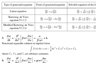
9.1. Equations Involving the First Derivative int 9.1.1. Korteweg–de Vries Equation ∂w∂t +a∂3
w ∂x3 +bw
∂w ∂x = 0
9.1.2. Cylindrical, Spherical, and Modified Korteweg–de Vries Equations 9.1.3. Generalized Korteweg–de Vries Equation ∂w∂t +a∂3
w ∂x3 +f(w)
∂w ∂x = 0
9.1.4. Equations Reducible to the Korteweg–de Vries Equation 9.1.5. Equations of the Form ∂w∂t +a∂∂x3w3 +f w,
∂w ∂x
= 0
9.1.6. Equations of the Form ∂w∂t +a∂3
w
∂x3 +F x,t,w,∂w
∂x
= 0
9.1.7. Burgers–Korteweg–de Vries Equation and Other Equations 9.2. Equations Involving the Second Derivative int
9.2.1. Equations with Quadratic Nonlinearities 9.2.2. Other Equations
9.3. Hydrodynamic Boundary Layer Equations
9.3.1. Steady Hydrodynamic Boundary Layer Equations for a Newtonian Fluid 9.3.2. Steady Boundary Layer Equations for Non-Newtonian Fluids
9.3.3. Unsteady Boundary Layer Equations for a Newtonian Fluid 9.3.4. Unsteady Boundary Layer Equations for Non-Newtonian Fluids 9.3.5. Related Equations
9.4. Equations of Motion of Ideal Fluid (Euler Equations) 9.4.1. Stationary Equations
9.4.2. Nonstationary Equations
9.5. Other Third-Order Nonlinear Equations
9.5.1. Equations Involving Second-Order Mixed Derivatives 9.5.2. Equations Involving Third-Order Mixed Derivatives 9.5.3. Equations Involving∂∂x3w3 and
∂3
10. Fourth Order Equations
10.1. Equations Involving the First Derivative int 10.1.1. Equations of the Form ∂w∂t =a∂4
10.2. Equations Involving the Second Derivative int 10.2.1. Boussinesq Equation and Its Modifications 10.2.2. Equations with Quadratic Nonlinearities 10.2.3. Other Equations
10.3. Equations Involving Mixed Derivatives 10.3.1. Kadomtsev–Petviashvili Equation
10.3.2. Stationary Hydrodynamic Equations (Navier–Stokes Equations) 10.3.3. Nonstationary Hydrodynamic Equations (Navier–Stokes equations) 10.3.4. Other Equations
11. Equations of Higher Orders
11.1. Equations Involving the First Derivative intand Linear in the Highest Derivative 11.1.1. Fifth-Order Equations
11.2. General Form Equations Involving the First Derivative int 11.2.1. Equations of the Form ∂w∂t =F w,∂w∂x,. . .,∂
11.3. Equations Involving the Second Derivative int 11.3.1. Equations of the Form ∂
2
11.3.3. Equations of the Form ∂ 2
11.4.1. Equations Involving Mixed Derivatives 11.4.2. Equations Involving ∂∂xnwn and
∂m
w ∂ym
Supplements. Exact Methods for Solving Nonlinear Partial Differential Equations
S.1. Classification of Second-Order Semilinear Partial Differential Equations in Two Independent Variables
S.2.1. Point Transformations S.2.2. Hodograph Transformation
S.2.3. Contact Transformations. Legendre and Euler Transformations S.2.4. B¨acklund Transformations. Differential Substitutions
S.3. Traveling-Wave Solutions and Self-Similar Solutions. Similarity Methods S.3.1. Preliminary Remarks
S.3.2. Traveling-Wave Solutions. Invariance of Equations Under Translations
S.3.3. Self-Similar Solutions. Invariance of Equations Under Scaling Transformations S.3.4. Exponential Self-Similar Solutions. Equations Invariant Under Combined
Translation and Scaling
S.4. Method of Generalized Separation of Variables S.4.1. Introduction
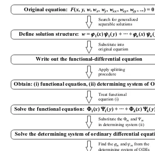
S.4.2. Structure of Generalized Separable Solutions
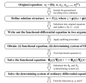
S.4.3. Solution of Functional-Differential Equations by Differentiation S.4.4. Solution of Functional-Differential Equations by Splitting
S.4.5. Simplified Scheme for Constructing Generalized Separable Solutions S.4.6. Titov–Galaktionov Method
S.5. Method of Functional Separation of Variables S.5.1. Structure of Functional Separable Solutions S.5.2. Special Functional Separable Solutions S.5.3. Differentiation Method
S.5.4. Splitting Method. Reduction to a Functional Equation with Two Variables S.5.5. Solutions of Some Nonlinear Functional Equations and Their Applications
S.6. Generalized Similarity Reductions of Nonlinear Equations
S.6.1. Clarkson–Kruskal Direct Method: a Special Form for Similarity Reduction S.6.2. Clarkson–Kruskal Direct Method: the General Form for Similarity Reduction S.6.3. Some Modifications and Generalizations
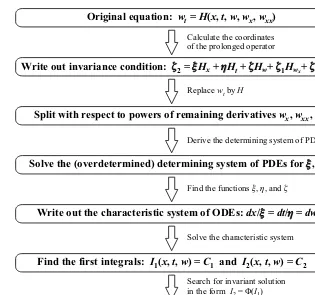
S.7. Group Analysis Methods
S.7.1. Classical Method for Symmetry Reductions S.7.2. Nonclassical Method for Symmetry Reductions
S.8. Differential Constraints Method S.8.1. Description of the Method
S.8.2. First-Order Differential Constraints
S.8.3. Second- and Higher-Order Differential Constraints
S.8.4. Connection Between the Differential Constraints Method and Other Methods
S.9. Painlev´e Test for Nonlinear Equations of Mathematical Physics
S.9.1. Movable Singularities of Solutions of Ordinary Differential Equations
S.9.2. Solutions of Partial Differential Equations with a Movable Pole. Description of the Method
S.9.3. Examples of the Painlev´e Test Applications
S.10. Inverse Scattering Method S.10.1. Lax Pair Method
S.10.2. Method Based on the Compatibility Condition for Two Linear Equations S.10.3. Method Based on Linear Integral Equations
S.11. Conservation Laws
S.11.1. Basic Definitions and Examples
S.12. Hyperbolic Systems of Quasilinear Equations S.12.1. Conservation Laws. Some Examples
S.12.2. Cauchy Problem, Riemann Problem, and Initial-Boundary Value Problem S.12.3. Characteristic Lines. Hyperbolic Systems. Riemann Invariants
S.12.4. Self-Similar Continuous Solutions. Rarefaction Waves S.12.5. Shock Waves. Rankine–Hugoniot Jump Conditions
S.12.6. Evolutionary Shocks. Lax Condition (Various Formulations) S.12.7. Solutions for the Riemann Problem
S.12.8. Initial-Boundary Value Problems of Special Form S.12.9. Examples of Nonstrict Hyperbolic Systems
AUTHORS
Andrei D. Polyanin, Ph.D., D.Sc., is a noted scientist of broad interests, who works in various areas of mathematics, mechanics, and chemical engineering sciences.
A. D. Polyanin graduated from the Department of Mechanics and Mathematics of the Moscow State University in 1974. He re-ceived his Ph.D. degree in 1981 and D.Sc. degree in 1986 at the Institute for Problems in Mechanics of the Russian (former USSR) Academy of Sciences. Since 1975, A. D. Polyanin has been a member of the staff of the Institute for Problems in Mechanics of the Russian Academy of Sciences. He is a member of the Russian National Committee on Theoretical and Applied Mechanics.
Professor Polyanin is an author of 33 books in English, Russian, German, and Bulgarian, as well as over 120 research papers and three patents. He has written a number of fundamental handbooks, including A. D. Polyanin and V. F. Zaitsev, Handbook of Exact Solutions for Ordinary Differential Equations, CRC Press, 1995 and 2002; A. D. Polyanin and A. V. Manzhirov,Handbook of Inte-gral Equations, CRC Press, 1998; A. D. Polyanin,Handbook of Linear Partial Differential Equations for Engineers and Scientists, Chapman & Hall/CRC Press, 2002; A. D. Polyanin, V. F. Zaitsev, and A. Moussiaux,Handbook of First Order Partial Differential Equations, Taylor & Francis, 2002; and A. D. Polyanin and V. F. Zaitsev,Handbook of Nonlinear Mathematical Physics Equations, Fizmatlit, 2002. Professor Polyanin is Editor of the book seriesDifferential and Integral Equa-tions and Their ApplicaEqua-tions, Taylor & Francis, London, andPhysical and Mathematical Reference Literature, Fizmatlit, Moscow.
In 1991, A. D. Polyanin was awarded a Chaplygin Prize of the Russian Academy of Sciences for his research in mechanics. In 2001, he received an award from the Ministry of Education of the Russian Federation.
Address:Institute for Problems in Mechanics, RAS, 101 Vernadsky Avenue, Building 1, 119526 Moscow, Russia
E›mail:[email protected]
Valentin F. Zaitsev, Ph.D., D.Sc.,is a noted scientist in the fields of ordinary differential equations, mathematical physics, and non-linear mechanics.
V. F. Zaitsev graduated from the Radio Electronics Faculty of the Leningrad Polytechnical Institute (now Saint-Petersburg Tech-nical University) in 1969 and received his Ph.D. degree in 1983 at the Leningrad State University. His Ph.D. thesis was devoted to the group approach to the study of some classes of ordinary differential equations. In 1992, Professor Zaitsev received his Doctor of Sci-ences degree; his D.Sc. thesis was dedicated to the discrete-group analysis of ordinary differential equations.
In 1971–1996, V. F. Zaitsev worked in the Research Institute for Computational Mathematics and Control Processes of the St. Pe-tersburg State University. Since 1996, Professor Zaitsev has been a member of the staff of the Russian State Pedagogical University (St. Petersburg).
Professor Zaitsev has made important contributions to new methods in the theory of ordinary and partial differential equations. He is an author of more than 130 scientific publications, including 18 books and one patent.
Address:Russian State Pedagogical University, 48 Naberezhnaya reki Moiki, 191186 Saint-Petersburg, Russia
FOREWORD
Nonlinear partial differential equations are encountered in various fields of mathematics, physics, chemistry, and biology, and numerous applications.
Exact (closed-form) solutions of differential equations play an important role in the proper understanding of qualitative features of many phenomena and processes in various areas of natural science. Exact solutions of nonlinear equations graphically demonstrate and allow unraveling the mechanisms of many complex nonlinear phenomena such as spatial localization of transfer processes, multiplicity or absence steady states under various conditions, existence of peaking regimes and many others. Furthermore, simple solutions are often used in teaching many courses as specific examples illustrating basic tenets of a theory that admit mathematical formulation.
Even those special exact solutions that do not have a clear physical meaning can be used as “test problems” to verify the consistency and estimate errors of various numerical, asymptotic, and approximate analytical methods. Exact solutions can serve as a basis for perfecting and testing computer algebra software packages for solving differential equations. It is significant that many equations of physics, chemistry, and biology contain empirical parameters or empirical functions. Exact solutions allow researchers to design and run experiments, by creating appropriate natural conditions, to determine these parameters or functions.
This book contains more than 1600 nonlinear mathematical physics equations and nonlinear partial differential equations and their solutions. A large number of new exact solutions to nonlinear equations are described. Equations of parabolic, hyperbolic, elliptic, mixed, and general types are discussed. Second-, third-, fourth-, and higher-order nonlinear equations are considered. The book presents exact solutions to equations of heat and mass transfer, wave theory, nonlinear mechanics, hydrodynamics, gas dynamics, plasticity theory, nonlinear acoustics, combustion theory, nonlinear optics, theoretical physics, differential geometry, control theory, chemical engineering sciences, biology, and other fields.
Special attention is paid to general-form equations that depend on arbitrary functions; exact solutions of such equations are of principal value for testing numerical and approximate methods. Almost all other equations contain one or more arbitrary parameters (in fact, this book deals with whole families of partial differential equations), which can be fixed by the reader at will.In total, the handbook contains significantly more nonlinear PDE’s and exact solutions than any other book currently available.
The supplement of the book presents exact analytical methods for solving nonlinear mathemati-cal physics equations. When selecting the material, the authors have given a pronounced preference to practical aspects of the matter; that is, to methods that allow effectively “constructing” exact solutions. Apart from the classical methods, the book also describes wide-range methods that have been greatly developed over the last decade (the nonclassical and direct methods for symmetry reductions, the differential constraints method, the method of generalized separation of variables, and others). For the reader’s better understanding of the methods, numerous examples of solv-ing specific differential equations and systems of differential equations are given throughout the book.
For the convenience of a wide audience with different mathematical backgrounds, the authors tried to do their best, wherever possible, to avoid special terminology. Therefore, some of the methods are outlined in a schematic and somewhat simplified manner, with necessaryreferences made to books where these methods are considered in more detail. Many sections were written so that they could be read independently from each other. This allows the reader to quickly get to the heart of the matter.
courses and lectures on nonlinear mathematical physics equations for graduate and postgraduate students. Furthermore, the books may be used as a database of test problems for numerical and approximate methods for solving nonlinear partial differential equations.
We would like to express our deep gratitude to Alexei Zhurov for fruitful discussions and valuable remarks.
The authors hope that this book will be helpful for a wide range of scientists, university teachers, engineers, and students engaged in the fields of mathematics, physics, mechanics, control, chemistry, and engineering sciences.
SOME NOTATIONS AND REMARKS
Latin Characters
C1,C2,. . . are arbitrary constants;
r,ϕ,z cylindrical coordinates,r=px2+y2 andx=rcosϕ,y=rsinϕ;
r,θ,ϕ spherical coordinates,r=px2+y2+z2 andx=rsinθcosϕ,y=sinθsinϕ,z=rcosθ;
t time (t≥ 0);
w unknown function (dependent variable);
x,y,z space (Cartesian) coordinates;
x1,. . .,xn Cartesian coordinates inn-dimensional space.
Greek Characters
∆ Laplace operator; in two-dimensional case,∆= ∂x∂22 +
∂2
∂y2;
in three-dimensional case,∆= ∂x∂22 +
∂2
∂y2 +
∂2
∂z2; inn-dimensional case,∆=
n
P
k=1
∂2
∂x2
k ;
∆∆ biharmonic operator; in two-dimensional case,∆∆= ∂x∂44 + 2
∂4
∂x2∂y2 +
∂4
∂y4.
Brief Notation for Derivatives
wx=
∂w ∂x, wt=
∂w
∂t , wxx= ∂2w
∂x2, wxt=
∂2w
∂x∂t, wtt= ∂2w
∂t2 , . . . (partial derivatives);
f′
x=
df dx, f
′′
xx=
d2f
dx2, fxxx′′′ =
d3f
dx3, fxxxx′′′′ =
d4f
dx4, f
(n)
x =
dnf
dxn (derivatives forf =f(x)).
Brief Notation for Differential Operators
∂x=
∂
∂x, ∂y = ∂
∂y, ∂t= ∂
∂t, ∂w= ∂
∂w (differential operators inx,y,t, andw);
Dx= ∂
∂x +wx ∂ ∂w +wxx
∂ ∂wx
+wxt ∂
∂wt
+· · · (total differential operator inx);
Dt= ∂
∂t +wt ∂ ∂w+wxt
∂ ∂wx
+wtt ∂
∂wt
+· · · (total differential operator int). In the last two relations,wis assumed to be dependent onxandt,w=w(x,t).
Remarks
1. The book presents solutions of the following types:
(a) expressible in terms of elementary functions explicitly, implicitly, or parametrically; (b) expressible in terms of elementary functions and integrals of elementary functions;
(c) expressible in terms of elementary functions, functions involved in the equation (if the equation contains arbitrary functions), and integrals of the equation functions and/or other elementary functions;
(d) expressible in terms of ordinary differential equations or finite systems of ordinary differential equations;
The book also deals with solutions described by equations with fewer new variables than those in the original equations. An expression that solves an equations in three independent variables and is determined by an equation in two independent variables will be called a two-dimensional solution.
3. As a rule, the book does not present simple solutions that depend on only one of the variables involved in the original equation.
4. Equations are numbered separately in each subsection. When referencing a particular equa-tion, we use a notation like 3.1.2.5, which implies equation 5 from Subsection 3.1.2.
5. If a formula or a solution contains an expression like f(x)
a− 2, it is often not stated that the
assumptiona≠ 2is implied.
6. Though incomplete, very simple and graphical classification of solutions by their appearance is used in the book. For equations in two independent variables,xandt, and one unknown,w, the solution name and structure are as follows (xandtin the solutions below can be swapped):
No. Solution name Solution structure
1 Traveling-wave solution∗ w=F(z), z=αx+βt, αβ≠ 0
2 Additive separable solution w=ϕ(x)+ψ(t)
3 Multiplicative separable solution w=ϕ(x)ψ(t)
4 Self-similar solution∗∗ w=tαF(z), z=xtβ
5 Generalized self-similar solution w=ϕ(t)F(z), z=xψ(t)
6 Generalized traveling-wave solution w=F(z), z=ϕ(t)x+ψ(t)
7 Generalized separable solution w=ϕ1(x)ψ1(t)+· · ·+ϕn(x)ψn(t)
8 Functional separable solution w=F(z), z=ϕ1(x)ψ1(t)+· · ·+ϕn(x)ψn(t)
∗For uniformity of presentation, we also use this term in the cases where the variabletplays the role of a spatial coordinate. ∗∗Sometimes, a solution of the formw=¯tαF(z), z=x¯¯tβ, where ¯x=x+C
1and ¯t=t+C2, will also be called a self-similar solution.
7. The present book does not consider first-order nonlinear partial differential equations. For these equations, see Kamke (1965), Rhee, Aris, and Amundson (1986, 1989), and Polyanin, Zaitsev, and Moussiaux (2002).
8. ODE and PDE are conventional abbreviations for ordinary differential equation and partial differential equation, respectively.
✂✁
This symbol indicates references to literature sources whenever:
(a) at least one of the solutions was obtained in the cited source (even though the solution contained “correctable” misprints in signs or coefficients);
Chapter 1
Parabolic Equations
with One Space Variable
1.1. Equations with Power-Law Nonlinearities
1.1.1. Equations of the Form
∂w
∂t
=
a ∂
2w
∂x
2+
bw
+
cw
21. ∂w ∂t =a
∂2w
∂x2 +bw 2.
1◦. Supposew(x,t) is a solution of this equation. Then the function
w1=C12w(C1x+C2,C12t+C3),
whereC1,C2, andC3are arbitrary constants, is also a solution of the equation.
2◦. Traveling-wave solution (λis an arbitrary constant):
w=w(z), z=x+λt,
where the functionw(z) is determined by the autonomous ordinary differential equation
aw′′
zz−λw′z+bw
2= 0
.
3◦. Self-similar solution:
w=t−1u(ξ), ξ=xt−1/2,
where the functionu(ξ) is determined by the ordinary differential equation
au′′
ξξ+ 12ξu′ξ+u+bu2= 0.
2. ∂w ∂t =
∂2w
∂x2 +aw(1 –w).
Fisher equation. This equation arises in heat and mass transfer, combustion theory, biology, and ecology. For example, it describes the mass transfer in a two-component medium at rest with a volume chemical reaction of quasi-first order. The kinetic functionf(w)=aw(1 −w) models also an autocatalytic chain reaction in combustion theory.
This is a special case of equation 1.1.3.2 withm= 2.
1◦. Supposew(x,t) is a solution of the equation in question. Then the functions
w1=w( x+C1,t+C2),
2◦. Traveling-wave solutions (Cis an arbitrary constant):
w(x,t)=1 +Cexp −56at✁
1 6
√
6a x−2,
w(x,t)=−1 +Cexp −56at✁
1 6
√
6a x−2,
w(x,t)= 1 + 2Cexp −
5 6at✁
1 6
√
−6a x
1 +Cexp −56at✁
1 6
√
−6a x2.
3◦. Traveling-wave solutions:
w(x,t)=✁ ξ
2ϕ
(ξ), ξ=C1exp 16 √
6a x+ 56at,
where the functionϕ(ξ) is defined implicitly by
ξ=
Z dϕ
p
✁ (4ϕ
3− 1) −C2,
andC1andC2are arbitrary constants. For the upper sign, the inversion of this relation corresponds
to the classical Weierstrass elliptic function,ϕ(ξ)=℘(ξ+C3,0,1).
4◦. The substitutionU = 1 −wleads to an equation of the similar form
∂U ∂t =
∂2U
∂x2 −aU(1 −U).
✂☎✄
References: M. J. Ablowitz and A. Zeppetella (1978), V. G. Danilov, V. P. Maslov, and K. A. Volosov (1995).
1.1.2. Equations of the Form
∂w
∂t
=
a ∂
2w
∂x
2+
b
0+
b
1w
+
b
2w
2+
b
3w
31. ∂w ∂t =a
∂2w
∂x2 –bw 3.
This is a special case of equation 1.1.2.5 withb0=b1=b2= 0.
1◦. Supposew(x,t) is a solution of the equation in question. Then the functions
w1=C1w(✁ C1x+C2,C
2 1t+C3),
whereC1,C2, andC3are arbitrary constants, are also solutions of the equation.
2◦. Solutions:
w(x,t)=✁
r
2a
b
2C1x+C2
C1x2+C2x+ 6aC1t+C3
.
3◦. Traveling-wave solution (λis an arbitrary constant):
w=w(z), z=x+λt,
where the functionw(z) is determined by the autonomous ordinary differential equation
aw′′
zz−λw′z−bw
3= 0
.
4◦. Self-similar solution:
w=t−1/2u
(ξ), ξ=xt−1/2
,
where the functionu(ξ) is determined by the ordinary differential equation
au′′
ξξ+ 12ξu′ξ+ 12u−bu 3= 0
. ✂☎✄
1.1. E P -L N 3
2. ∂w ∂t =
∂2w
∂x2 +aw–bw 3.
This is a special case of equation 1.1.2.5 withb0=b2= 0.
1◦. Supposew(x,t) is a solution of the equation in question. Then the functions
w1=✆ w(✆ x+C1,t+C2),
whereC1 andC2 are arbitrary constants, are also solutions of the equation (the signs are chosen
arbitrarily).
2◦. Solutions witha>0andb>0:
w=
r a b
C1exp 12 √
2a x−C2exp −12
√
2a x
C1exp 12 √
2a x+C2exp −12
√
2a x+C3exp −32at
,
w=
r a b
2C
1exp √
2a x+C2exp 12
√
2a x− 32at
C1exp √
2a x+C2exp 12
√
2a x− 3
2at
+C3
− 1
,
whereC1,C2, andC3are arbitrary constants.
3◦. Solution witha<0andb>0:
w=
r
|a|
b
sin 12√2|a|x+C1
cos 12√2|a|x+C1
+C2exp −32at
,
whereC1andC2are arbitrary constants.
4◦. Solution witha>0(generalizes the first solution of Item2◦):
w=C1exp 12 √
2a x+ 32at−C2exp −12
√
2a x+ 32atU(z),
z=C1exp 12 √
2a x+ 32at+C2exp −12
√
2a x+ 32at+C3,
whereC1,C2, andC3 are arbitrary constants, and the functionU = U(z) is determined by the
autonomous ordinary differential equation aU′′
zz = 2bU3 (whose solution can be written out in implicit form).
5◦. Solution witha<0(generalizes the solution of Item3◦):
w=exp 32atsin 21p2|a|x+C1
V(ξ),
ξ=exp 32atcos 21p2|a|x+C1
+C2,
whereC1andC2are arbitrary constants, and the functionV =V(ξ) is determined by the autonomous
ordinary differential equationaV′′
ξξ = −2bV3(whose solution can be written out in implicit form).
6◦. See also equation 1.1.3.2 withm= 3.
✝☎✞
References: F. Cariello and M. Tabor (1989), M. C. Nucci and P. A. Clarkson (1992).
3. ∂w ∂t =a
∂2w
∂x2 –bw 3–
cw2.
This is a special case of equation 1.1.2.5 withb1=b0= 0.
1◦. Traveling-wave solutions:
w(x,t)=
ct✆
r b
2ax+C
−1
,
2◦. Solutions:
Fitzhugh–Nagumo equation.This equation arises in population genetics and models the transmission of nerve impulses.
1◦. There are three stationary solutions: w=wk, wherew1 = 0,w2 = 1, andw3 =a. The linear
stability analysis shows that
if−1 ≤a<0: the solutionsw=a, w= 1are stable, w= 0is unstable; if 0<a<1: the solutionsw= 0,w= 1are stable, w=ais unstable.
There is a stationary nonhomogeneous solution that can be represented in implicit form (Aand
Bare arbitrary constants):
Z dw
2◦. Traveling-wave solutions (A,B, andCare arbitrary constants):
1.1. E P -L N 5
3◦. “Two-phase” solution:
w(x,t)= Aexp(z1)+aBexp(z2)
Aexp(z1)+Bexp(z2)+C
,
z1=✠
√
2 2 x+
1 2 −a
t, z2=✠
√
2 2 ax+a
1 2a− 1
t, whereA,B, andCare arbitrary constants.
4◦. The solutions of Item2◦are special cases of the traveling-wave solution
w(x,t)=w(ξ), ξ=x+λt,
whereλis an arbitrary constant, and the functionw(ξ) is determined by the autonomous ordinary differential equation
w′′
ξξ−λw′ξ =w(1 −w)(a−w). The substitutionw′
ξ =λy(w) leads to an Abel equation of the second kind:
yy′
w−y=λ
−2
aw−(a+ 1)w2+w3. The general solution of this equation witha= −1andλ=✠
3
√
2 can be found in Polyanin and Zaitsev
(2003).
5◦. Let us give two transformations that preserve the form of the original equation.
The substitutionu= 1 −wleads to an equation of the similar form with parametera1= 1 −a: ∂u
∂t = ∂2u
∂x2 −u(1 −u)(1 −a−u).
The transformation
v(z,τ)= 1 − 1
aw(x,t), τ=a 2t
, z=ax
leads to an equation of the similar form with parametera2= 1 −a−1: ∂v
∂τ = ∂2v
∂z2 −v(1 −v)
1 − 1
a −v
.
Therefore, ifw=w(x,t;a) is a solution of the equation in question, then the functions
w1 = 1 −w x,t; 1 −a
,
w2 =a−aw ax,a2t;1 −a−1
are also solutions of the equation. The abovesaid allows us to “multiply” exact solutions.
6◦. See also Example 1 in Subsection S.7.2.
✡☎☛
References for equation1.1.2.4: T. Kawahara and M. Tanaka (1983), M. C. Nucci and P. A. Clarkson (1992), N. H. Ibrag-imov (1994), V. F. Zaitsev and A. D. Polyanin (1996).
5. ∂w ∂t =a
∂2w
∂x2 +b0+b1w+b2w 2+b
3w3.
1◦. Solutions are given by
w(x,t)= β
F ∂F
∂x +λ, β =✠
r
−2a
b3
, (1)
whereλis any of the roots of the cubic equation
b3λ3+b2λ2+b1λ+b0= 0 (2)
Introduce the notation
p1= −3a, p2=β(b2+ 3b3λ), q1= − β
2a(b2+ 3b3λ), q2= −
1
2a(3b3λ
2+ 2
b2λ+b1). (3)
Four cases are possible.
1.1. Forq2≠ 0andq12≠ 4q2, we have
F(x,t)=C1exp(k1x+s1t)+C2exp(k2x+s2t)+C3, kn = −12q1☞
1 2
q q2
1− 4q2, sn = −kn2p1−knp2,
(4)
whereC1,C2, andC3are arbitrary constants;n= 1,2.
1.2. Forq2≠ 0andq12= 4q2, we have
F(x,t)=C1exp(kx+s1t)+C2(kx+s2t) exp(kx+s1t)+C3, k= −12q1, s1= −14p1q12+
1
2p2q1, s2= − 1 2p1q
2 1+
1 2p2q1.
1.3. Forq2= 0andq1≠ 0,
F(x,t)=C1(x−p2t)+C2exp[−q1x+q1(p2−p1q1)t]+C3.
1.4. Forq2=q1= 0,
F(x,t)=C1(x−p2t)2+C2(x−p2t)− 2C1p1t+C3.
Example. Let
a= 1, b0= 0, b1w+b2w 2
+b3w 3
= −bw(w−λ1)(w−λ2). By formulas (1)–(4) withλ= 0, one can obtain the solution
w(x,t)= C1λ1exp(z1)+C2λ2exp(z2) C1exp(z1)+C2exp(z2)+C3 ,
where
z1=✌
1 2
√
2b λ1x+ 1
2bλ1(λ1− 2λ2)t,
z2=✌
1 2
√
2b λ2x+12bλ2(λ2− 2λ1)t.
2◦. There is a traveling-wave solution, w=w(x+γt).
✍☎✎
References: V. G. Danilov and P. Yu. Sybochev (1991), N. A. Kudryashov (1993), P. A. Clarkson and E. L. Mansfield (1994).
1.1.3. Equations of the Form
∂w
∂t
=
a ∂
2w
∂x
2+
f
(w)
1. ∂w ∂t =a
∂2w
∂x2 +bw
k.
1◦. Supposew(x,t) is a solution of this equation. Then the functions
w1=C12w(☞ C k−1
1 x+C2,C12k−2t+C3),
whereC1,C2, andC3are arbitrary constants, are also solutions of the equation.
2◦. Traveling-wave solution:
w=w(z), z=x+λt,
whereλis an arbitrary constant and the functionw(z) is determined by the autonomous ordinary differential equation
aw′′
zz−λwz′ +bwk= 0.
3◦. Self-similar solution:
w=t1−1ku(ξ), ξ= √x
t,
where the functionu(ξ) is determined by the ordinary differential equation
au′′
ξξ+
1
2ξu
′
ξ+
1
k− 1u+bu
1.1. E P -L N 7
2. ∂w ∂t =
∂2w
∂x2 +aw+bw
m.
Kolmogorov–Petrovskii–Piskunov equation.This equation arises in heat and mass transfer, combus-tion theory, biology, and ecology.
1◦. Traveling-wave solutions:
w(x,t)=β+Cexp(λt✏ µx)
2
1−m, (1)
w(x,t)=−β+Cexp(λt✏ µx)
2
1−m, (2)
whereCis an arbitrary constant and the parametersλ,µ, andβare given by
λ= a(1 −m)(m+ 3)
2(m+ 1) , µ=
s
a(1 −m)2
2(m+ 1) , β=
r
−b
a.
2◦. Solutions (1) and (2) are special cases of a wider class of solutions, the class of traveling-wave
solutions:
w=w(z), z=✏ µx+λt. These are determined by the autonomous equation
µ2w′′
zz−λw′z+aw+bwm= 0. (3) For
µ=
s
a(m+ 3)2
2(m+ 1), λ=µ
2
(m≠✏ 1, m≠ −3)
the solution of equation (3) can be represented in parametric form as
z= m+ 3
m− 1lnf(ζ), w=ζ
f(ζ)
2
m−1,
where the functionf(ζ) is given by
f(ζ)=✏
Z C1−
4b
a(m− 1)2ζ
m+1 −1/2
dζ+C2,
andC1andC2are arbitrary constants.
3◦. By the change of variableU(w)=µ2λ−1w′
z, equation (3) can be reduced to an Abel equation of the second kind:
U U′
w−U=a1w+b1wm, a1= −aµ2λ−2, b1= −bµ2λ−2.
The books by Polyanin and Zaitsev (1995, 2003) present exact solutions of this equation for some values ofmanda1(b1is any).
✑☎✒
References: P. Kaliappan (1984), V. G. Danilov, V. P. Maslov, and K. A. Volosov (1995), V. F. Zaitsev and A. D. Polyanin (1996).
3. ∂w ∂t =
∂2w
∂x2 +aw+bw
m+
cw2m–1.
1◦. Traveling-wave solutions:
w(x,t)=β+Cexp(λt+µx)
1
1−m, (1)
whereCis an arbitrary constant and the parametersβ,λ, andµare determined by the system of algebraic equations
aβ2+bβ+c= 0
, (2)
µ2−(1 −m)λ+a(1 −m)2= 0, (3)
µ2−λ+
(1 −m)[2a+(b/β)= 0. (4) The quadratic equation (2) forβcan be solved independently. In the general case, system (2)–(4) gives four sets of the parameters, which generate four exact solutions of the original equation. ✓☎✔
Reference: V. F. Zaitsev and A. D. Polyanin (1996).
2◦. Solution (1) is a special case of a wider class of traveling-wave solutions,
w=w(z), z=x+σt, that are determined by the autonomous equation
w′′
zz−σw′z+aw+bwm+cw
2m−1= 0
. (5)
The substitutionU(w)=w′
zbrings (5) to the Abel equation
U U′
w−σU+aw+bwm+cw2m−1= 0,
whose general solutions for somem(no constraints are imposed ona,b, andc) can be found in the books by Polyanin and Zaitsev (1995, 2003).
3◦. The substitution
u=w1−m leads to an equation with quadratic nonlinearity:
u∂u ∂t =u
∂2u ∂x2 +
m
1 −m
∂u
∂x 2
+a(1 −m)u2+b
(1 −m)u+c(1 −m). (6) Solution (1) corresponds to a particular solution of (6) that has the formu=β+Cexp(ωt+µx). Fora= 0, equation (6) has also other traveling-wave solutions:
u(x,t)=(1 −m)
bt✕
r
− c
mx
+C.
4. ∂w ∂t =
∂2w
∂x2 +aw
m–1+
bmwm–mb2w2m–1. Traveling-wave solution:
w=w(z), z=x+λt,
whereλis an arbitrary constant and the functionw(z) is determined by the autonomous ordinary differential equation
w′′
zz−λwz′ +awm
−1+
bmwm−mb2w2m−1= 0. (1)
Forλ= 1, it can be shown that a one-parameter family of solutions to equation (1) satisfies the first-order equation
w′
z=w−bwm+
a
mb. (2)
Integrating (2) yields a solution in implicit form (Ais any):
Z dw
a+mbw−mb2wm =
1
mbz+A. (3)
In the special casea= 0, it follows from (3) that
1.1. E P -L N 9
1.1.4. Equations of the Form
∂w
∂t
=
a ∂
2w
∂x
2+
f
(x,
t,
w)
1. ∂w ∂t =a
∂2w
∂x2 +✖ 1(bx+ct) k+
✖ 2w n.
This is a special case of equation 1.6.1.2 withf(z,w)=s1zk+s2wn.
2. ∂w ∂t =a
∂2w
∂x2 +✖ (w+bx+ct) k.
This is a special case of equation 1.6.1.2 withf(z,w)=s(w+z)k.
3. ∂w ∂t =a
∂2w
∂x2 +✖ (bx+ct) k
wn.
This is a special case of equation 1.6.1.2 withf(z,w)=szkwn.
4. ∂w ∂t =a
∂2w
∂x2 +bt
nxmwk.
1◦. Supposew(x,t) is a solution of this equation. Then the function
w1 =C2n+m+2w(Ck−1x,C2k−2t),
whereCis an arbitrary constant, is also a solution of the equation.
2◦. Self-similar solution:
w=t 2n+m+2
2(1−k) u(ξ), ξ= √x
t,
where the functionu=u(ξ) is determined by the ordinary differential equation
au′′
ξξ+
1
2ξu
′
ξ+
2n+m+ 2
2(k− 1) u+bξ
muk= 0 .
5. ∂w ∂t =a
∂2w
∂x2 +✖ e bx+ct
wn.
This is a special case of equation 1.6.1.2 withf(z,w)=sezwn.
1.1.5. Equations of the Form
∂w
∂t
=
a ∂
2w
∂x
2+
f
(w)
∂w
∂x
+
g(w)
1. ∂w ∂t =a
∂2w
∂x2 +b
∂w
∂x +cw+k1w n1
+k2wn2.
This is a special case of equation 1.6.2.3 withf(t)=b. On passing fromt,xto the new variables
t,z=x+bt, one arrives at the simpler equation
∂w ∂t =a
∂2w
∂z2 +cw+k1w
n1+k
2wn2,
special cases of which are discussed in Subsections 1.1.1 to 1.1.3.
2. ∂w ∂t =
∂2w
∂x2 +w
∂w ∂x.
1◦. Supposew(x,t) is a solution of the equation in question. Then the function
w1=C1w(C1x+C1C2t+C3,C12t+C4)+C2,
whereC1,. . .,C4are arbitrary constants, is also a solution of the equation.
2◦. Solutions:
w(x,t)= A−x
B+t, w(x,t)=λ+ 2
x+λt+A, w(x,t)= 4x+ 2A
x2+Ax+ 2t+B, w(x,t)= 6(x
2+ 2t+A
)
x3+ 6xt+ 3Ax+B, w(x,t)= 2λ
1 +Aexp(−λ2t−λx),
w(x,t)= −λ+Aexp
A(x−λt)]−B
expA(x−λt)+B, w(x,t)= −λ+ 2AtanhA(x−λt)+B,
w(x,t)= λ
λ2t+A
2tanh
λx+B λ2t+A
−λx−B
,
w(x,t)= −λ+ 2AtanA(λt−x)+B,
w(x,t)= 2λcos(λx+A)
Bexp(λ2t)+sin(λx+A), w(x,t)= √ 2A
π(t+λ)exp
−(x+B)
2
4(t+λ)
Aerf
x+B
2√t+λ
+C
−1
,
whereA,B,C, andλare arbitrary constants, and erfz≡ √2
π Z z
0
exp(−ξ2)dξis the error function (also called the probability integral).
3◦. Other solutions can be obtained using the following formula (Hopf–Cole transformation):
w(x,t)= 2
u ∂u
∂x, (1)
whereu=u(x,t) is a solution of the linear heat equation
∂u ∂t =
∂2u
∂x2. (2)
For details about this equation, see the books Tikhonov and Samarskii (1990) and Polyanin (2002). ✗☎✘
References: E. Hopf (1950), J. Cole (1951).
Remark. The transformation (1) and equation 1.6.3.2, which is a generalized Burgers equation,
were encountered much earlier in Fortsyth (1906).
4◦. Cauchy problem. Initial condition:
w=f(x) at t= 0, −∞<x<∞. Solution:
w(x,t)= 2 ∂
∂xlnF(x,t),
where
F(x,t)= √1
4πt
Z ∞
−∞
exp
−(x−ξ)
2
4t −
1 2
Z ξ
0
f(ξ′)dξ′
dξ. ✗☎✘
1.1. E P -L N 11
5◦. The Burgers equation is connected with the linear heat equation (2) by the B ¨acklund
transfor-mation
∂u ∂x −
1
2uw= 0,
∂u ∂t −
1 2
∂(uw)
∂x = 0.
✙☎✚
References for equation1.1.5.2: J. M. Burgers (1948), O. V. Rudenko and C. I. Soluyan (1975), N. H. Ibragimov (1994), V. F. Zaitsev and A. D. Polyanin (1996).
3. ∂w ∂t =a
∂2w
∂x2 +bw
∂w ∂x.
Unnormalized Burgers equation.The scaling of the independent variablesx= a
bz,t= a
b2τleads to
an equation of the form 1.1.5.2:
∂w ∂τ =
∂2w ∂z2 +w
∂w ∂z.
4. ∂w ∂t =a
∂2w
∂x2 +bw
∂w ∂x +c. The transformation
w=u(z,t)+ct, z=x+ 12bct2
, leads to the Burgers equation 1.1.5.3:
∂u ∂t =a
∂2u ∂z2 +bu
∂u ∂z.
5. ∂w ∂t +σw
∂w ∂x =a
∂2w
∂x2 +bw.
1◦. Supposew(x,t) is a solution of this equation. Then the function
w1 =w x−C1σebt+C2,t+C3+Cbebt,
whereC1,C2, andC3are arbitrary constants, is also a solution of the equation.
2◦. Traveling-wave solution:
w=w(z), z=x+λt,
whereλis an arbitrary constant and the functionw(z) is determined by the autonomous ordinary differential equation
aw′′
zz−σww′z−λwz′ +bw= 0.
3◦. Degenerate solution:
w(x,t)= b(x+C1)
σ(1 +C2e−bt)
.
6. ∂w ∂t +σw
∂w ∂x =a
∂2w
∂x2 +b1w+b0.
1◦. Supposew(x,t) is a solution of this equation. Then the function
w1=w x−C1σeb1t+C2,t+C3
+Cb1eb1t,
whereC1,C2, andC3are arbitrary constants, is also a solution of the equation.
2◦. The transformation
w=u(z,t)− b0
b1
, z=x+σb0 b1
t, leads to a simpler equation of the form 1.1.5.5:
∂u ∂t +σu
∂u ∂z =a
7. ∂w ∂t =a
∂2w
∂x2 +bw
∂w ∂x +
b2
9aw(w–k)(w+k). Solution:
w= k(−1 +C1e
4λx)
1 +C1e4λx+C2e2λx+bkλt
, λ= bk
12a,
whereC1andC2are arbitrary constants.
✛☎✜
Private communication: K. A. Volosov (2000).
8. ∂w ∂t +σw
∂w ∂x =a
∂2w
∂x2 +b0+b1w+b2w 2+
b3w3.
Solutions of the equation are given by
w(x,t)= β
z ∂z
∂x +λ. (1)
Here,βandλare any of the roots of the respective quadratic and cubic equations
b3β2+σβ+ 2a= 0, b3λ3+b2λ2+b1λ+b0= 0,
and the specific form ofz=z(x,t) depends on the equation coefficients.
1◦. Caseb3≠ 0.Introduce the notation:
p1= −βσ− 3a, p2=λσ+βb2+ 3βλb3, q1= −
βb2+ 3βλb3
βσ+ 2a , q2= −
3b3λ2+ 2b2λ+b1
βσ+ 2a .
Four cases are possible.
1.1. Forq2≠ 0andq21≠ 4q2, we have
z(x,t)=C1exp(k1x+s1t)+C2exp(k2x+s2t)+C3, kn= −12q1✢
1 2
q q2
1− 4q2, sn= −k 2
np1−knp2,
whereC1,C2, andC3are arbitrary constants;n= 1,2.
1.2. Forq2≠ 0andq21= 4q2,
z(x,t)=C1exp(kx+s1t)+C2(kx+s2t) exp(kx+s1t)+C3, k= −12q1, s1= −14p1q12+
1
2p2q1, s2= − 1 2p1q
2 1+
1 2p2q1.
1.3. Forq2= 0andq1≠ 0,
z(x,t)=C1(x−p2t)+C2exp[−q1x+q1(p2−p1q1)t]+C3.
1.4. Forq2=q1= 0,
z(x,t)=C1(x−p2t)2+C2(x−p2t)− 2C1p1t+C3.
2◦. Caseb
3= 0andb2≠ 0.Solutions are given by (1) with β= −2a
σ, z(x,t)=C1+C2exp
Ax+A
b1σ
2b2
+ 2ab2
σ
t
, A= σ(b1+ 2b2λ)
2ab2
,
whereλis a root of the quadratic equationb2λ2+b1λ+b0= 0.
3◦. Caseb3=b2= 0.See equations 1.1.5.4–1.1.5.6.
✛☎✜
1.1. E P -L N 13
9. ∂w ∂t =a
∂2w
∂x2 +bw
m∂w ∂x.
1◦. Supposew(x,t) is a solution of this equation. Then the function
w1=C1w C1mx+C2,C12mt+C3
,
whereC1,C2, andC3are arbitrary constants, is also a solution of the equation.
2◦. Traveling-wave solution:
w(x,t)=
Cexp
−λm
a z
+ b
λ(m+ 1)
−1/m
, z=x+λt,
whereCandλare arbitrary constants. A wider family of traveling-wave solutions is presented in 1.6.3.7 forf(w)=bwm.
3◦. There is a self-similar solution of the form
w(ξ,t)= |t|−21mϕ(ξ), ξ=x|t|−12.
1.1.6. Equations of the Form
∂w
∂t
=
a ∂
2w
∂x
2+
f
(x,
t,
w)
∂w
∂x
+
g(x,
t,
w)
1. ∂w ∂t =a
∂2w
∂x2 + (bx+c)
∂w ∂x +
✣ w k.
This is a special case of equation 1.6.2.1 withf(w)=swk.
1◦. Supposew(x,t) is a solution of this equation. Then the function
w1=w(x+C1e−bt,t+C2),
whereC1andC2are arbitrary constants, is also a solution of the equation.
2◦. Generalized traveling-wave solution:
w=w(z), z=x+C1e−bt,
where the functionw(z) is determined by the ordinary differential equation
aw′′
zz+bzwz′ +swk = 0. 2. ∂w
∂t =a ∂2w
∂x2 +bt
n∂w
∂x +cw+k1w m1
+k2wm2.
This is a special case of equation 1.6.2.3 withf(t)=btn. On passing fromt,xto the new variables
t,z=x+ b
n+ 1t
n+1
, one arrives at the simpler equation
∂w ∂t =a
∂2w
∂z2 +cw+k1w
m1+k
2wm2,
special cases of which are discussed in Subsections 1.1.1 to 1.1.3.
3. ∂w ∂t +
k
tw+bw ∂w
∂x =a ∂2w
∂x2.
Modified Burgers equation.
1◦. Supposew(x,t) is a solution of the equation in question. Then the functions
w1 =C1w(C1x+C2,C12t),
w2 =w(x−bC3t1−k,t)+C3(1 −k)t−k if k≠ 1, w3 =w(x−bC3ln|t|,t)+C3t−1 if k= 1,
2◦. Degenerate solution linear inx:
w(x,t)= (1 −k)x+C1
C2tk+bt
if k≠ 1,
w(x,t)= x+C1
t(C2+bln|t|)
if k= 1, whereC1andC2are arbitrary constants.
3◦. Self-similar solution:
w(x,t)=u(z)t−1/2
, z=xt−1/2
,
where the functionu=u(z) is determined by the ordinary differential equation
au′′
zz+ 12z−bu
u′
z+ 12 −k
u= 0.
4. ∂w ∂t +bw
∂w ∂x =a
1
x ∂ ∂x
x∂w ∂x
– w x2
.
Cylindrical Burgers equation. The variablexplays the role of the radial coordinate. Solution:
w(x,t)= −2a
b
1
θ ∂θ ∂x,
where the functionθ=θ(x,t) satisfies the linear heat equation with axial symmetry
∂θ ∂t =
a x
∂ ∂x
x∂θ
∂x
. ✤☎✥
Reference: S. Nerney, E. J. Schmahl, and Z. E. Musielak (1996).
5. ∂w ∂t +bw
∂w ∂x =a
∂2w
∂x2 +cx
k∂w ∂x +ckx
k–1
w.
Solution:
w(x,t)= −2a
b
1
θ ∂θ ∂x,
where the functionθ=θ(x,t) satisfies the linear equation
∂θ ∂t =a
∂2θ ∂x2 +cx
k∂θ
∂x.
6. ∂w ∂t =a
∂2w
∂x2 +bw
∂w
∂x +c(x+ ✦ t)
k.
This is a special case of equation 1.6.3.2 withf(x,t)=c(x+st)k.
7. ∂w ∂t =a
∂2w ∂x2 +bw
∂w ∂x +cx
k+ ✦ t
n.
This is a special case of equation 1.6.3.2 withf(x,t)=cxk+stn.
8. ∂w ∂t =a
∂2w
∂x2 + (bx+cw
k)∂w ∂x.
1◦. Supposew(x,t) is a solution of this equation. Then the function
w1=w(x+C1e−bt,t+C2),
whereC1andC2are arbitrary constants, is also a solution of the equation.
2◦. Generalized traveling-wave solution:
w=w(z), z=x+C1e−bt,
where the functionw(z) is determined by the ordinary differential equation
aw′′
1.1. E P -L N 15
9. ∂w ∂t =a
∂2w
∂x2 + (bw
m+ ct+✧ )
∂w ∂x.
This is a special case of equation 1.6.3.11 withf(w)=bwm,g(t)=ct+s, andh(w)= 0. On passing fromt,xto the new variablest,z=x+ 1
2ct 2+st
, we obtain an equation of the form 1.1.5.9:
∂w ∂t =a
∂2w ∂z2 +bw
m∂w
∂z.
10. ∂w ∂t =a
∂2w
∂x2 + (bw
m+
ctk)∂w ∂x.
This is a special case of equation 1.6.3.11 withf(w)=bwm,g(t)=ctk, andh(w)= 0. On passing fromt,xto the new variablest,z =x+ c
k+ 1t
k+1
, we obtain an equation of the form 1.1.5.9:
∂w ∂t =a
∂2w ∂z2 +bw
m∂w
∂z.
11. ∂w ∂t =a
∂2w
∂x2 +✧ 1(bx+ct) k
wn∂w ∂x +
✧ 2(bx+ct) p
wq.
This is a special case of equation 1.6.3.13 withf(z,w)=s1zkwnandg(z,w)=s2zpwq.
1.1.7. Equations of the Form
∂w
∂t
=
a ∂
2w
∂x
2+
b
∂w
∂x
2+
f
(x,
t,
w)
1. ∂w ∂t =a
∂2w
∂x2 +b
∂w
∂x
2
.
1◦. Solutions:
w(x)= a
b ln|Ax+B| +C, w(x,t)=A2bt
★ Ax+B,
w(x,t)= −(x+A)
2
4bt −
a
2blnt+B,
w(x,t)= a
b ln|x 2+ 2
at+Ax+B| +C,
w(x,t)= a
b ln|x
3+ 6axt+Ax+B| +C
,
w(x,t)= a
b ln|x
4+ 12ax2t+ 12a2t2+A| +B
,
w(x,t)= −a
2λ2
b t+ a
b ln|cos(λx+A)| +B,
whereA,B,C, andλare arbitrary constants.
2◦. The substitution
w(x,t)= a
b ln|u(x,t)|
leads to the linear heat equation
∂u ∂t =a
∂2u ∂x2.