Chapter 20
Nonlinear Ordinary Differential Equations
This chapter is concerned with initial value problems for systems of ordinary differ-ential equations. We have already dealt with the linear case in Chapter 9, and so here our emphasis will be on nonlinear phenomena and properties, particularly those with physical relevance. Finding a solution to a differential equation may not be so important if that solution never appears in the physical model represented by the system, or is only realized in exceptional circumstances. Thus, equilibrium solutions, which correspond to configura-tions in which the physical system does not move, only occur in everyday situaconfigura-tions if they are stable. An unstable equilibrium will not appear in practice, since slight perturbations in the system or its physical surroundings will immediately dislodge the system far away from equilibrium.
Of course, very few nonlinear systems can be solved explicitly, and so one must typ-ically rely on a numerical scheme to accurately approximate the solution. Basic methods for initial value problems, beginning with the simple Euler scheme, and working up to the extremely popular Runge–Kutta fourth order method, will be the subject of the final section of the chapter. However, numerical schemes do not always give accurate results, and we breifly discuss the class of stiff differential equations, which present a more serious challenge to numerical analysts.
Without some basic theoretical understanding of the nature of solutions, equilibrium points, and stability properties, one would not be able to understand when numerical so-lutions (even those provided by standard well-used packages) are to be trusted. Moreover, when testing a numerical scheme, it helps to have already assembled a repertoire of nonlin-ear problems in which one already knows one or more explicit analytic solutions. Further tests and theoretical results can be based on first integrals (also known as conservation laws) or, more generally, Lyapunov functions. Although we have only space to touch on these topics briefly, but, we hope, this will whet the reader’s appetite for delving into this subject in more depth. The references [19,59,93,103,109] can be profitably consulted.
20.1. First Order Systems of Ordinary Differential Equations.
Scalar Ordinary Differential Equations
As always, when confronted with a new problem, it is essential to fully understand the simplest case first. Thus, we begin with a single scalar, first order ordinary differential equation
du
dt =F(t, u). (20.1)
In many applications, the independent variable t represents time, and the unknown func-tion u(t) is some dynamical physical quantity. Throughout this chapter, all quantities are assumed to be real. (Results on complex ordinary differential equations can be found in [102].) Under appropriate conditions on the right hand side (to be formalized in the following section), the solution u(t) is uniquely specified by its value at a single time,
u(t0) =u0. (20.2)
The combination (20.1–2) is referred to as an initial value problem, and our goal is to devise both analytical and numerical solution strategies.
A differential equation is calledautonomous if the right hand side does not explicitly depend upon the time variable:
du
dt =F(u). (20.3)
All autonomous scalar equations can be solved by direct integration. We divide both sides by F(u), whereby
1
F(u)
du dt = 1,
and then integrate with respect to t; the result is Z
1
F(u)
du dt dt=
Z
dt=t+k,
where k is the constant of integration. The left hand integral can be evaluated by the change of variables that replaces t by u, whereby du= (du/dt)dt, and so
Z 1
F(u)
du dt dt=
Z du
F(u) =G(u),
where G(u) indicates a convenient anti-derivative† of the function 1/F(u). Thus, the
solution can be written in implicit form
G(u) =t+k. (20.4)
If we are able to solve the implicit equation (20.4), we may thereby obtain the explicit solution
u(t) =H(t+k) (20.5)
† Technically, a second constant of integration should appear here, but this can be absorbed
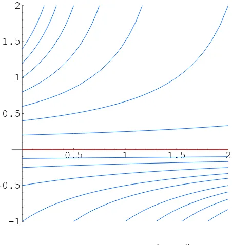
0.5 1 1.5 2
-1 -0.5 0.5 1 1.5 2
Figure 20.1. Solutions to
u=u2.
in terms of the inverse function H = G−1. Finally, to satisfy the initial condition (20.2), we set t = t0 in the implicit solution formula (20.4), whereby G(u0) =t0 +k. Therefore, the solution to our initial value problem is
G(u)−G(u0) =t−t0, or, explicitly, u(t) =H t−t0+G(u0). (20.6)
Remark: A more direct version of this solution technique is to rewrite the differential equation (20.3) in the “separated form”
du
F(u) =dt,
in which all terms involving u, including its differential du, are collected on the left hand side of the equation, while all terms involvingt and its differential are placed on the right, and then formally integrate both sides, leading to the same implicit solution formula:
G(u) =
Z du
F(u) = Z
dt=t+k. (20.7)
Before completing our analysis of this solution method, let us run through a couple of elementary examples.
Example 20.1. Consider the autonomous initial value problem
du dt =u
2, u(t
0) =u0. (20.8)
To solve the differential equation, we rewrite it in the separated form
du
u2 = dt, and then integrate both sides: − 1
u =
Z
du
Solving the resulting algebraic equation for u, we deduce the solution formula
u=− 1
t+k . (20.9)
To specify the integration constant k, we evaluate u at the initial timet0; this implies
u0 =− 1
t0+k , so that k =−
1
u0 −t0.
Therefore, the solution to the initial value problem is
u= u0
1−u0(t−t0). (20.10)
Figure 20.1 shows the graphs of some typical solutions.
Ast approaches the critical valuet⋆ =t0+ 1/u0 from below, the solution “blows up”, meaning u(t) → ∞ as t → t⋆. The blow-up time t⋆ depends upon the initial data — the larger u0 >0 is, the sooner the solution goes off to infinity. If the initial data is negative,
u0 < 0, the solution is well-defined for all t > t0, but has a singularity in the past, at
t⋆ =t
0+ 1/u0 < t0. The only solution that exists for all positive and negative time is the constant solution u(t)≡0, corresponding to the initial conditionu0 = 0.
In general, the constant equilibrium solutions to an autonomous ordinary differential equation, also known as itsfixed points, play a distinguished role. Ifu(t)≡u⋆ is a constant solution, thendu/dt ≡0, and hence the differential equation (20.3) implies thatF(u⋆) = 0. Therefore, the equilibrium solutions coincide with the roots of the function F(u). In point of fact, since we divided by F(u), the derivation of our formula for the solution (20.7) assumed that we were not at an equilibrium point. In the preceding example, our final solution formula (20.10) happens to include the equilibrium solution u(t) ≡ 0, corresponding tou0 = 0, but this is a lucky accident. Indeed, the equilibrium solution does not appear in the “general” solution formula (20.9). One must typically take extra care that equilibrium solutions do not elude us when utilizing this basic integration method.
Example 20.2. Although a population of people, animals, or bacteria consists of individuals, the aggregate behavior can often be effectively modeled by a dynamical system that involves continuously varying variables. As first proposed by the English economist Thomas Malthus in 1798, the population of a species grows, roughly, in proportion to its size. Thus, the number of individuals N(t) at time t satisfies a first order differential equation of the form
dN
dt =ρ N, (20.11)
where the proportionality factor ρ = β − δ measures the rate of growth, namely the difference between the birth rate β ≥ 0 and the death rate δ ≥ 0. Thus, if births exceed deaths, ρ >0, and the population increases, whereas if ρ <0, more individuals are dying and the population shrinks.
(8.1) that we solved at the beginning of Chapter 8. The solutions satisfy the Malthusian exponential growth law N(t) = N0eρ t, where N
0 = N(0) is the initial population size. Thus, if ρ >0, the population grows without limit, while ifρ < 0, the population dies out, so N(t) → 0 as t → ∞, at an exponentially fast rate. The Malthusian population model provides a reasonably accurate description of the behavior of an isolated population in an environment with unlimited resources.
In a more realistic scenario, the growth rate will depend upon the size of the population as well as external environmental factors. For example, in the presence of limited resources, relatively small populations will increase, whereas an excessively large population will have insufficient resources to survive, and so its growth rate will be negative. In other words, the growth rate ρ(N) > 0 when N < N⋆, while ρ(N) < 0 when N > N⋆, where the carrying capacity N⋆ > 0 depends upon the resource availability. The simplest class of functions that satifies these two inequalities are of the form ρ(N) = µ(N⋆ −N), where
µ >0 is a positive constant. This leads us to the nonlinear population model
dN
dt =µ N(N
⋆−N). (20.12)
In deriving this model, we assumed that the environment is not changing over time; a dynamical environment would require a more complicated non-autonomous differential equation.
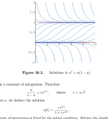
Before analyzing the solutions to the nonlinear population model, let us make a pre-liminary change of variables, and set u(t) = N(t)/N⋆, so that u represents the size of the population in proportion to the carrying capacity N⋆. A straightforward computation shows that u(t) satisfies the so-called logistic differential equation
du
dt =λ u(1−u), u(0) =u0, (20.13)
where λ = N⋆µ, and, for simplicity, we assign the initial time to be t0 = 0. The logis-tic differential equation can be viewed as the continuous counterpart of the logislogis-tic map (19.19). However, unlike its discrete namesake, the logistic differential equation is quite sedate, and its solutions easily understood.
First, there are two equilibrium solutions: u(t)≡0 and u(t)≡1, obtained by setting the right hand side of the equation equal to zero. The first represents a nonexistent population with no individuals and hence no reproduction. The second equilibrium solution corresponds to a static population N(t)≡N⋆ that is at the ideal size for the environment, so deaths exactly balance births. In all other situations, the population size will vary over time.
To integrate the logistic differential equation, we proceed as above, first writing it in the separated form
du
u(1−u) =λ dt. Integrating both sides, and using partial fractions,
2 4 6 8 10
-1 -0.5 0.5 1 1.5 2
Figure 20.2. Solutions to u′ =u(1−u).
where k is a constant of integration. Therefore
u
1−u =c e
λ t, where c= ±ek.
Solving for u, we deduce the solution
u(t) = c e λ t
1 +c eλ t . (20.14)
The constant of integration is fixed by the initial condition. Solving the algebraic equation
u0 =u(0) = c
1 +c yields c=
u0
1−u0 .
Substituting the result back into the solution formula (20.14) and simplifying, we find
u(t) = u0e λ t
1−u0+u0eλ t . (20.15)
The resulting solutions are illustrated in Figure 20.2. Interestingly, while the equilibrium solutions are not covered by the integration method, they reappear in the final solution formula, corresponding to initial data u0 = 0 and u0 = 1 respectively. However, this is a lucky accident, and cannot be anticipated in more complicated situations.
slow down the growth rate, and eventually the population saturates at the equilibrium value. On the other hand, if u0 > 1, the population is too large to be sustained by the available resources, and so dies off until it reaches the same saturation value. If u0 = 0, then the solution remains at equilibriumu(t)≡0. Finally, when u0 <0, the solution only exists for a finite amount of time, with
u(t) −→ −∞ as t −→ t⋆ = 1
λlog
1− u1
0
.
Of course, this final case does appear in the physical world, since we cannot have a negative population!
The separation of variables method used to solve autonomous equations can be stra-ightforwardly extended to a special class of non-autonomous equations. A separable ordi-nary differential equation has the form
du
dt =a(t)F(u), (20.16)
in which the right hand side is the product of a function oft and a function of u. To solve the equation, we rewrite it in the separated form
du
F(u) =a(t)dt.
Integrating both sides leads to the solution in implicit form
G(u) = Z
du F(u) =
Z
a(t)dt=A(t) +k. (20.17)
The integration constant k is then fixed by the initial condition. And, as before, one must properly account for any equilibrium solutions, whenF(u) = 0.
Example 20.3. Let us solve the particular initial value problem
du
dt = (1−2t)u, u(0) = 1. (20.18)
We begin by writing the differential equation in separated form
du
u = (1−2t)dt.
Integrating both sides leads to
logu = Z
du u =
Z
(1−2t)dt=t−t2+k,
where k is the constant of integration. We can readily solve for
u(t) =c et−t2,
where c = ±ek. The latter formula constitutes the general solution to the differential equation, and happens to include the equilibrium solutionu(t)≡0 when c= 0. The given initial condition requires that c= 1, and hence u(t) =et−t2
0.5 1 1.5 2 2.5 3 0.25
0.5 0.75 1 1.25 1.5
Figure 20.3. Solution to the Initial Value Problem
u = (1−2t)u, u(0) = 1.
First Order Systems
A first order system of ordinary differential equations has the general form
du1
dt =F1(t, u1, . . . , un), · · ·
dun
dt =Fn(t, u1, . . . , un). (20.19)
The unknowns u1(t), . . . , un(t) are scalar functions of the real variable t, which usually represents time. We shall write the system more compactly in vector form
du
dt =F(t,u), (20.20)
whereu(t) = (u1(t), . . . , un(t) )T, andF(t,u) = (F1(t, u1, . . . , un), . . . , Fn(t, u1, . . . , un) )T is a vector-valued function of n+ 1 variables. By a solution to the differential equation, we mean a vector-valued function u(t) that is defined and continuously differentiable on an interval a < t < b, and, moreover, satisfies the differential equation on its interval of definition. Each solution u(t) serves to parametrize a curve C ⊂ Rn, also known as a trajectory or orbit of the system.
In this chapter, we shall concentrate on initial value problems for such first order systems. The general initial conditions are
u1(t0) =a1, u2(t0) =a2, · · · un(t0) =an, (20.21)
or, in vectorial form,
u(t0) =a (20.22)
A system of differential equations is calledautonomous if the right hand side does not explicitly depend upon the time t, and so takes the form
du
dt =F(u). (20.23)
One important class of autonomous first order systems are the steady state fluid flows. Here F(u) = v represents the fluid velocity vector field at the position u. The solution u(t) to the initial value problem (20.23, 22) describes the motion of a fluid particle that starts at position a at time t0. The differential equation tells us that the fluid velocity at each point on the particle’s trajectory matches the prescribed vector field. Additional details can be found in Chapter 16 and Appendices A and B.
An equilibrium solution is constant: u(t) ≡ u⋆ for all t. Thus, its derivative must vanish, du/dt≡0, and hence, every equilibrium solution arises as a solution to the system of algebraic equations
F(u⋆) =0 (20.24)
prescribed by the vanishing of the right hand side of the system (20.23).
Example 20.4. A predator-prey system is a simplified ecological model of two species: the predators which feed on the prey. For example, the predators might be lions roaming the Serengeti and the prey zebra. We letu(t) represent the number of prey, andv(t) the number of predators at time t. Both species obey a population growth model of the form (20.11), and so the dynamical equations can be written as
du
dt =ρ u,
dv
dt =σ v, (20.25)
where the growth rates ρ, σ may depend upon the other species. The more prey, i.e., the larger u is, the faster the predators reproduce, while a lack of prey will cause them to die off. On the other hand, the more predators, the faster the prey are consumed and the slower their net rate of growth.
If we assume that the environment has unlimited resources for the prey, which, bar-ring drought, is probably valid in the case of the zebras, then the simplest model that incorporates these assumptions is the Lotka–Volterra system
du
dt =α u−δ u v,
dv
dt =−β v+γ u v, (20.26)
corresponding to growth rates ρ = α−δ v, σ = −β +γ u. The parameters α, β, γ, δ >
0 are all positive, and their precise values will depend upon the species involved and how they interact, as indicated by field data, combined with, perhaps, educated guesses. In particular, α represents the unrestrained growth rate of the prey in the absence of predators, while −β represents the rate that the predators die off in the absence of their prey. The nonlinear terms model the interaction of the two species: the rate of increase in the predators is proportional to the number of available prey, while the rate of decrese in the prey is proportional to the number of predators. The initial conditions u(t0) = u0,
We will discuss the integration of the Lotka–Volterra system (20.26) in Section 20.3. Here, let us content ourselves with determining the possible equilibria. Setting the right hand sides of the system to zero leads to the nonlinear algebraic system
0 =α u−δ u v=u(α−δ v), 0 =−β v+γ u v =v(−β +γ u).
Thus, there are two distinct equilibria, namely
u⋆1 =v⋆1 = 0, u⋆2 =β/γ, v2⋆ =α/δ.
The first is the uninteresting (or, rather catastropic) situation where there are no animals — no predators and no prey. The second is a nontrivial solution in which both populations maintain a steady value, for which the birth rate of the prey is precisely sufficient to continuously feed the predators. Is this a feasible solution? Or, to state the question more mathematically, is this a stable equilibrium? We shall develop the tools to answer this question below.
Higher Order Systems
A wide variety of physical systems are modeled by nonlinear systems of differential equations depending upon second and, occasionally, even higher order derivatives of the unknowns. But there is an easy device that will reduce any higher order ordinary differ-ential equation or system to an equivalent first order system. “Equivalent” means that each solution to the first order system uniquely corresponds to a solution to the higher order equation and vice versa. The upshot is that, for all practical purposes, one only needs to analyze first order systems. Moreover, the vast majority of numerical solution algorithms are designed for first order systems, and so to numerically integrate a higher order equation, one must place it into an equivalent first order form.
We have already encountered the main idea in our discussion of the phase plane approach to second order scalar equations
d2u
We introduce a new dependent variablev = du
dt . Since dv
dt = d2u
dt2 , the functionsu, vsatisfy the equivalent first order system order system, then its first component u(t) defines a solution to the scalar equation, which establishes their equivalence. The basic initial conditions u(t0) = u0, v(t0) = v0, for the first order system translate into a pair of initial conditionsu(t0) =u0,
u(t0) =v0, specifying the value of the solution and its first order derivative for the second order equation.
Similarly, given a third order equation
we set The variables u, v, w satisfy the equivalent first order system
du
The general technique should now be clear.
Example 20.5. The forced van der Pol equation
d2u dt2 + (u
2
−1) du
dt +u =f(t) (20.29)
arises in the modeling of an electrical circuit with a triode whose resistance changes with the current, [EE]. It also arises in certain chemical reactions, [odz], and wind-induced motions of structures, [odz]. To convert the van der Pol equation into an equivalent first order system, we set v=du/dt, whence
du dt =v,
dv
dt =f(t)−(u
2−1)v−u, (20.30)
is the equivalent phase plane system.
Example 20.6. The Newtonian equations for a massm moving in a potential force field are a second order system of the form
m d
2u
dt2 =−∇F(u)
in which u(t) = (u(t), v(t), w(t) )T represents the position of the mass and F(u) =
F(u, v, w) the potential function. In components,
m d
For example, a planet moving in the sun’s gravitational field satisfies the Newtonian system for the gravitational potential
where α depends on the masses and the universal gravitational constant. (This simplified model ignores all interplanetary forces.) Thus, the mass’ motion in such a gravitational force field follows the solution to the second order Newtonian system
The same system of ordinary differential equations describes the motion of a charged particle in a Coulomb electric force field, where the sign of α is positive for attracting opposite charges, and negative for repelling like charges.
To convert the second order Newton equations into a first order system, we setv =
u to be the mass’ velocity vector, with components
p= du
One of Newton’s greatest acheivements was to solve this system in the case of the cen-tral gravitational potential (20.32), and thereby confirm the validity of Kepler’s laws of planetary motion.
Finally, we note that there is a simple device that will convert any non-autonomous system into an equivalent autonomous system involving one additional variable. Namely, one introduces an extra coordinate u0 = t to represent the time, which satisfies the el-ementary differential equation du0/dt = 1 with initial condition u0(t0) = t0. Thus, the original system (20.19) can be written in the autonomous form
du0
For example, the autonomous form of the forced van der Pol system (20.30) is
du0 in which u0 represents the time variable.
20.2. Existence, Uniqueness, and Continuous Dependence.
It goes without saying that there is no general analytical method that will solve all differential equations. Indeed, even relatively simple first order, scalar, non-autonomous ordinary differential equations cannot be solved in closed form. For example, the solution to the particular Riccati equation
du dt =u
2+t (20.36)
cannot be written in terms of elementary functions, although the method of Exercise can be used to obtain a formula that relies on Airy functions, cf. (Ai , Bi ). TheAbel equation
du dt =u
fares even worse, since its general solution cannot be written in terms of even standard special functions — although power series solutions can be tediously ground out term by term. Understanding when a given differential equation can be solved in terms of elementary functions or known special functions is an active area of contemporary research, [32]. In this vein, we cannot resist mentioning that the most important class of exact solution techniques for differential equations are those based on symmetry. An introduction can be found in the author’s graduate level monograph [147]; see also [40,108].
Existence
Before worrying about how to solve a differential equation, either analytically, qual-itatively, or numerically, it behooves us to try to resolve the core mathematical issues of existence and uniqueness. First, does a solution exist? If, not, it makes no sense trying to find one. Second, is the solution uniquely determined? Otherwise, the differential equation probably has scant relevance for physical applications since we cannot use it as a predictive tool. Since differential equations inevitably have lots of solutions, the only way in which we can deduce uniqueness is by imposing suitable initial (or boundary) conditions.
Unlike partial differential equations, which must be treated on a case-by-case basis, there are complete general answers to both the existence and uniqueness questions for initial value problems for systems of ordinary differential equations. (Boundary value problems are more subtle.) While obviously important, we will not take the time to present the proofs of these fundamental results, which can be found in most advanced textbooks on the subject, including [19,93,103,109].
Let us begin by stating the Fundamental Existence Theorem for initial value problems associated with first order systems of ordinary differential equations.
Theorem 20.7. Let F(t,u) be a continuous function. Then the initial value prob-lem†
du
dt =F(t,u), u(t0) =a, (20.38)
admits a solutionu=f(t)that is, at least, defined for nearby times, i.e., when|t−t0|< δ
for some δ >0.
Theorem 20.7 guarantees that the solution to the initial value problem exists — at least for times sufficiently close to the initial instant t0. This may be the most that can be said, although in many cases the maximal interval α < t < β of existence of the solution might be much larger — possibly infinite, −∞ < t < ∞, resulting in a global solution. The interval of existence of a solution typically depends upon both the equation and the particular initial data. For instance, even though its right hand side is defined everywhere, the solutions to the scalar initial value problem (20.8) only exist up until time 1/u0, and so, the larger the initial data, the shorter the time of existence. In this example, the only global solution is the equilibrium solutionu(t)≡0. It is worth noting that this short-term
† If F(t,u) is only defined on a subdomain Ω ⊂ Rn+1, then we must assume that the point
existence phenomenon does not appear in the linear regime, where, barring singularities in the equation itself, solutions to a linear ordinary differential equation are guaranteed to exist for all time.
In practice, one always extends a solutions to its maximal interval of existence. The Existence Theorem 20.7 implies that there are only two possible ways in whcih a solution cannot be extended beyond a timet⋆: Either
(i) the solution becomes unbounded: ku(t)k → ∞ as t →t⋆, or
(ii) if the right hand sideF(t,u) is only defined on a subset Ω⊂Rn+1, then the solution u(t) reaches the boundary ∂Ω as t →t⋆.
If neither occurs in finite time, then the solution is necessarily global. In other words, a solution to an ordinary differential equation cannot suddenly vanish into thin air.
Remark: The existence theorem can be readily adapted to any higher order system of ordinary differential equations through the method of converting it into an equivalent first order system by introducing additional variables. The appropriate initial conditions guaranteeing existence are induced from those of the corresponding first order system, as in the second order example (20.27) discussed above.
Uniqueness and Smoothness
As important as existence is the question of uniqueness. Does the initial value problem have more than one solution? If so, then we cannot use the differential equation to predict the future behavior of the system from its current state. While continuity of the right hand side of the differential equation will guarantee that a solution exists, it is not quite sufficient to ensure uniqueness of the solution to the initial value problem. The difficulty can be appreciated by looking at an elementary example.
Example 20.8. Consider the nonlinear initial value problem
du dt =
5 3u
2/5, u(0) = 0. (20.39)
Since the right hand side is a continuous function, Theorem 20.7 assures us of the existence of a solution — at least for t close to 0. This autonomous scalar equation can be easily solved by the usual method:
Z 3
5
du u2/5 =u
3/5 =t+c, and so u = (t+c)5/3.
Substituting into the initial condition implies thatc= 0, and henceu(t) =t5/3is a solution to the initial value problem.
On the other hand, since the right hand side of the differential equation vanishes at
0.5 1 1.5 2 0.5
1 1.5 2
Figure 20.4. Solutions to the Differential Equation
u = 53u2/5.
valid! Worse yet, there are, in fact, an infinite number of solutions to the initial value problem. For any a >0, the function
u(t) =
0, 0
≤t ≤a,
(t−a)5/3, t≥a, (20.40)
is differentiable everywhere, even at t =a. (Why?) Moreover, it satisfies both the differ-ential equation and the initial condition, and hence defines a solution to the initial value problem. Several of these solutions are plotted in Figure 20.4.
Thus, to ensure uniqueness of solutions, we need to impose a more stringent condition, beyond mere continuity. The proof of the following basic uniqueness theorem can be found in the above references.
Theorem 20.9. If F(t,u)∈ C1 is continuously differentiable, then there exists one and only one solution† to the initial value problem (20.38).
Thus, the difficulty with the differential equation (20.39) is that the function F(u) = 5
3u2/5, although continuous everywhere, is not differentiable at u = 0, and hence the Uniqueness Theorem 20.9 does not apply. On the other hand, F(u) is continuously differ-entiable away fromu= 0, and so any nonzero initial conditionu(t0) =u0 6= 0 will produce a unique solution — for as long as it remains away from the problematic value u= 0.
Blanket Hypothesis: From now on, all differential equations must satisfy the unique-ness criterion that their right hand side is continuously differentiable.
While continuous differentiability is sufficient to guarantee uniqueness of solutions, the smoother the right hand side of the system, the smoother the solutions. Specifically:
Theorem 20.10. If F∈Cn for n≥1, then any solution to the system
u =F(t,u)
is of class u∈Cn+1. IfF(t,u) is an analytic function, then all solutionsu(t)are analytic.
The basic outline of the proof of the first result is clear: Continuity of u(t) (which is a basic prerequiste of any solution) implies continuity of F(t,u(t)), which means
u is continuous and hence u ∈ C1. This in turn implies F(t,u(t)) =
u is a continuously differentiable of t, and so u ∈ C2. And so on, up to order n. The proof of analyticity follows from a detailed analysis of the power series solutions, [102]. Indeed, the analytic result underlies the method of power series solutions of ordinary differential equations, developed in detail in Appendix series.
Uniqueness has a number of particularly important consequences for the solutions to autonomous systems, i.e., those whoe right hand side does not explicitly depend upon t. Throughout the remainder of this section, we will deal with an autonomous system of ordinary differential equations
du
dt =F(u), where F∈C
1, (20.41)
whose right hand side is defined and continuously differentiable for all u in a domain Ω ⊂ Rn. As a consequence, each solution u(t) is, on its interval of existence, uniquely determined by its initial data. Autonomy of the differential equation is an essential hy-pothesis for the validity of the following properties.
The first result tells us that the solution trajectories of an autonomous system do not vary over time.
Proposition 20.11. If u(t) is the solution to the autonomous system (20.41) with initial condition u(t0) = u0, then the solution to the initial value problem ue(t1) = u0 is
e
u(t) =u(t−t1+t0).
Proof: Let ue(t) = u(t−t1 +t0), where u(t) is the original solution. In view of the chain rule and the fact that t1 and t0 are fixed,
d
dtue(t) = du
dt (t−t1+t0) =F u(t−t1 +t0)
=F ue(t),
and hence eu(t) is also a solution to the system (20.41). Moreover,
e
u(t1) =u(t0) =u0
has the indicated initial conditions, and hence, by uniqueness, must be the one and only
solution to the latter initial value problem. Q.E.D.
One particularly important consequence of uniqueness is that a solution u(t) to an autonomous system is either stuck at an equilibrium for all time, or is always in motion. In other words, either
u ≡ 0, in the case of equilibrium, or, otherwise,
u 6= 0 wherever defined.
Proposition 20.12. Let u⋆ be an equilibrium for the autonomous system (20.41), soF(u⋆) =0. Ifu(t) is any solution such thatu(t⋆) =u⋆ at some timet⋆, then u(t)≡u⋆
is the equilibrium solution.
Proof: We regard u(t⋆) =u⋆ as initial data for the given solution u(t) at the initial timet⋆. SinceF(u⋆) =0, the constant function u⋆(t)≡u⋆ is a solution of the differential equation that satisfies the same initial conditions. Therefore, by uniqueness, it coincides
with the solution in question. Q.E.D.
In other words, it is mathematically impossible for a solution to reach an equilibrium position in a finite amount of time — although it may well approach equilibrium in an asymptotic fashion as t → ∞; see Proposition 20.15 below for details. Physically, this observation has the interesting and physically counterintuitive consequence that a mathe-matical system never actually attains an equilibrium position! Even at very large times, there is always some very slight residual motion. In practice, though, once the solution gets sufficiently close to equilibrium, we are unable to detect the motion, and the physical system has, in all but name, reached its stationary equilibrium configuration. And, of course, the inherent motion of the atoms and molecules not included in such a simplified model would hide any infinitesimal residual effects of the mathematical solution. Without uniqueness, the result is false. For example, the function u(t) = (t−t⋆)5/3 is a solution to the scalar ordinary differential equation (20.39) that reaches the equilibrium point u⋆ = 0 in a finite time t=t⋆.
Continuous Dependence
In a real-world applications, initial conditions are almost never known exactly. Rather, experimental and physical errors will only allow us to say that their values are approxi-mately equal to those in our mathematical model. Thus, to retain physical relevance, we need to be sure that small errors in our initial measurements do not induce a large change in the solution. A similar argument can be made for any physical parameters, e.g., masses, charges, spring stiffnesses, frictional coefficients, etc., that appear in the differential equa-tion itself. A slight change in the parameters should not have a dramatic effect on the solution.
Mathematically, what we are after is a criterion ofcontinuous dependence of solutions upon both initial data and parameters. Fortunately, the desired result holds without any additional assumptions, beyond requiring that the parameters appear continuously in the differential equation. We state both results in a single theorem.
Theorem 20.13. Consider an initial value problem problem
du
in which the differential equation and/or the initial conditions depend continuously on one or more parameters µ = (µ1, . . . , µk). Then the unique† solution u(t,µ) depends continuously upon the parameters.
Example 20.14. Let us look at a perturbed version
du
dt =α u
2, u(0) =u 0+ε,
of the initial value problem that we considered in Example 20.1. We regard ε as a small perturbation of our original initial datau0, and αas a variable parameter in the equation. The solution is
u(t, ε) = u0 +ε
1−α(u0 +ε)t. (20.43)
Note that, where defined, this is a continuous function of both parameters α, ε. Thus, a small change in the initial data, or in the equation, produces a small change in the solution — at least for times near the initial time.
Continuous dependence does not preclude nearby solutions from eventually becoming far apart. Indeed, the blow-up time t⋆ = 1/α(u0+ε) for the solution (20.43) depends upon both the initial data and the parameter in the equation. Thus, as we approach the singularity, solutions that started out very close to each other will get arbitrarily far apart; see Figure 20.1 for an illustration.
An even simpler example is the linear model of exponential growth
u = α u when
α >0. A very tiny change in the initial conditions has a negligible short term effect upon the solution, but over longer time intervals, the differences between the two solutions will be dramatic. Thus, the “sensitive dependence” of solutions on initial conditions already appears in very simple linear equations. For similar reasons, sontinuous dependence does not prevent solutions from exhibiting chaotic behavior. Further development of these ideas can be found in [7,57] and elsewhere.
As an application, let us show that if a solution to an autonomous system converges to a single limit point, then that point is necessarily an equilibrium solution. Keep in mind that, owing to uniqueness of solutions, the limiting equilibrium cannot be mathematically achieved in finite time, but only as a limit as time goes to infinity.
Proposition 20.15. Let u(t) be a solution to the autonomous system
u = F(u), with F ∈ C1, such that lim
t→ ∞ u(t) =u
⋆. Then u⋆ is an equilibrium solution, and so F(u⋆) =0.
Proof: Letv(t,a) denote the solution to the initial value problem
v=F(v), v(0) =a. (We use a different letter to avoid confusion with the given solution u(t).) Theorem 20.13 implies that v(t,a) is a continuous function of the initial position a. and hence v(t,u(s)) is a continuous function ofs ∈R. Since lim
s→ ∞ u(s) =u
⋆, we have
lim
s→ ∞ v(t,u(s)) =v(t,u
⋆).
On the other hand, since the system is autonomous, Proposition 20.11 (or, equivalently, Exercise ) implies that v(t,u(s)) =u(t+s), and hence
lim
s→ ∞ v(t,u(s)) = lims→ ∞ u(t+s) =u
⋆.
Equating the preceding two limit equations, we conclude that v(t,u⋆) = u⋆ for all t, and hence the solution with initial valuev(0) =u⋆ is an equilibrium solution. Q.E.D.
The same conclusion holds if we run time backwards: if lim
t→ −∞ u(t) =u⋆, then u⋆ is
also an equilibrium point. When they exist, solutions that start and end at equilibrium points play a particularly role in the dynamics, and are known asheteroclinic, or, if the start and end equilibria are the same, homoclinic orbits. Of course, limiting equilibrium points are but one of the possible long term behaviors of solutions to nonlinear ordinary differential equations, which can also become unbounded in finite or infinite time, or approach periodic orbits, known aslimit cycles, or become completely chaotic, depending upon the nature of the system and the initial conditions. Resolving the long term behavior os solutions is one of the many challenges awaiting the detailed analysis of any nonlinear ordinary differential equation.
20.3. Stability.
Once a solution to a system of ordinary differential equations has settled down, its limiting value is an equilibrium solution; this is the content of Proposition 20.15. However, not all equilibria appear in this fashion. The only steady state solutions that one directly observes in a physical system are the stable equilibria. Unstable equilibria are hard to sustain, and will disappear when subjected to even the tiniest perturbation, e.g., a breath of air, or outside traffic jarring the experimental apparatus. Thus, finding the equilibrium solutions to a system of ordinary differential equations is only half the battle; one must then understand their stability properties in order to characterize those that can be realized in normal physical circumstances.
We will focus our attention on autonomous systems
u= F(u)
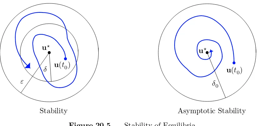
whose right hand sides are at least continuously differentiable, so as to ensure the unique-ness of solutions to the initial value problem. If every solution that starts out near a given equilibrium solution tends to it, the equilibrium is called asymptotically stable. If the solutions that start out nearby stay nearby, then the equilibrium isstable. More formally:
Definition 20.16. An equilibrium solution u⋆ to an autonomous system of first order ordinary differential equations is called
• stable if for every (small) ε > 0, there exists a δ > 0 such that every solution u(t) having initial conditions within distance δ > ku(t0)−u⋆k of the equilibrium rmains within distance ε > ku(t)−u⋆k for all t ≥t0.
δ ε
u⋆
u(t0)
Stability
δ0
u⋆
u(t0)
Asymptotic Stability
Figure 20.5. Stability of Equilibria.
Thus, although solutions nearby a stable equilibrium may drift slightly farther away, they must remain relatively close. In the case of asymptotic stability, they will eventually return to equilibrium. This is illustrated in Figure 20.5
Example 20.17. As we saw, the logistic differential equation
du
dt =λ u(1−u)
has two equilibrium solutions, corresponding to the two roots of the quadratic equation
λ u(1−u) = 0. The solution graphs in Figure 20.1 illustrate the behavior of the solutions. Observe that the first equilibrium solution u⋆
1 = 0 is unstable, since all nearby solutions go away from it at an exponentially fast rate. On the other hand, the other equilibrium solution u⋆
2 = 1 is asymptotically stable, since any solution with initial condition 0 < u0 tends to it, again at an exponentially fast rate.
Example 20.18. Consider an autonomous (meaning constant coefficient) homoge-neous linear planar system
du
dt =a u+b v,
dv
dt =c u+d v,
with coefficient matrix A =
a b
c d
Stability of Scalar Differential Equations
Before looking at any further examples, we need to develop some basic mathematical tools for investigating the stability of equilibria. We begin at the beginning. The stability analysis for first order scalar ordinary differential equations
du
dt =F(u) (20.44)
is particularly easy. The first observation is that all non-equilibrium solutions u(t) are strictly monotone functions, meaning they are either always increasing or always decreas-ing. Indeed, when F(u) > 0, then (20.44) implies that the derivative
u > 0, and hence
u(t) is increasing at such a point. Vice versa, solutions are decreasing at any point where
F(u)<0. SinceF(u(t)) depends continuously ont, any non-monotone solution would have to pass through an equilibrium value where F(u⋆) = 0, in violation of Proposition 20.12. This proves the claim.
As a consequence of monotonicity, there are only three possible behaviors for a non-equilibrium solution:
(a) it becomes unbounded at some finite time: |u(t)| → ∞ as t→t⋆; or (b) it exists for all t≥t0, but becomes unbounded ast → ∞; or
(c) it exists for all t ≥ t0 and has a limiting value, u(t) → u⋆ as t → ∞, which, by Proposition 20.15 must be an equilibrium point.
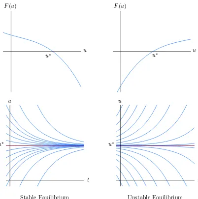
Let us look more carefully at the last eventuality. Suppose u⋆ is an equilibrium point, so F(u⋆) = 0. Suppose that F(u) >0 for all u lying slightly below u⋆, i.e., on an interval of the form u⋆−δ < u < u⋆. Any solution u(t) that starts out on this interval,
u⋆ −δ < u(t0) < u⋆ must be increasing. Moreover, u(t)< u⋆ for all t since, according to Proposition 20.12, the solution cannot pass through the equilibrium point. Therefore,u(t) is a solution of type (c). It must have limiting value u⋆, since by assumption, this is the only equilibrium solution it can increase to. Therefore, in this situation, the equilibrium pointu⋆ isasymptotically stable from below: solutions that start out slightly below return to it in the limit. On the other hand, if F(u) < 0 for all u slightly below u⋆, then any solution that starts out in this regime will be monotonically decreasing, and so will move downwards, away from the equilibrium point, which is thus unstable from below.
By the same reasoning, if F(u) < 0 for u slightly above u⋆, then solutions starting out there will be monotonically decreasing, bounded from below by u⋆, and hence have no choice but to tend to u⋆ in the limit. Under this condition, the equilibrium point is asymptotically stable from above. The reverse inequality, F(u) > 0, corresponds to solutions that increase away from u⋆, which is hence unstable from above. Combining the two stable cases produces the basic asymptotic stability criterion for scalar ordinary differential equations.
Theorem 20.19. A equilibrium pointu⋆ of an autonomous scalar differential equa-tion is asymptotically stable if and only if F(u)>0 for u⋆−δ < u < u⋆ and F(u)<0 for
u F(u)
u⋆ u
F(u)
u⋆
u
t u⋆
Stable Equilibrium
u
t u⋆
Unstable Equilibrium Figure 20.6. Equilibria of Scalar Ordinary Differential Equations.
In other words, if F(u) switches sign from positive to negative as u increases through the equilibrium point, then the equilibrium is asymptotically stable. If the inequalities are reversed, and F(u) goes from negative to positive, then the equilibrium point is unstable. The two cases are illustrated in Figure 20.6. An equilibrium point where F(u) is of one sign on both sides, e.g., the point u⋆ = 0 for F(u) = u2, is stable from one side, and unstable from the other; in Exercise you are asked to analyze such cases in detail.
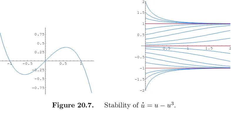
Example 20.20. Consider the differential equation
du
dt =u−u
3. (20.45)
Solving the algebraic equation F(u) = u−u3 = 0, we find that the equation has three equilibria: u⋆1 = −1, u⋆2 = 0, u⋆3 = +1, As u increases, the graph of the function F(u) =
u−u3 switches from positive to negative at the first equilibrium point u⋆
-1 -0.5 0.5 1
-0.75 -0.5 -0.25 0.25 0.5 0.75
0.5 1 1.5 2
-2 -1.5 -1 -0.5 0.5 1 1.5 2
Figure 20.7. Stability of
u=u−u3.
establishing the instability of the second equilibrium. The final equilibrium u⋆3 = +1 is stable because F(u) again changes from negative to positive there.
With this information in hand, we are able to completely characterize the behavior of all solutions to the system. Any solution with negative initial condition, u0 < 0, will end up, asymptotically, at the first equilibrium, u(t)→ −1 ast → ∞. Indeed, ifu0 <−1, then
u(t) is monotonically increasing to −1, while if −1 < u0 < 0, the solution is decreasing towards −1. On the other hand, if u0 > 0, the corresponding solution ends up at the other stable equilibrium, u(t) →+1; those with 0< u0 < 1 are monotonically increasing, while those with u0 >1 are decreasing. The only solution that does not end up at either −1 or +1 as t → ∞ is the unstable equilibrium solution u(t) ≡ 0. Any perturbation of it, no matter how tiny, will force the solutions to choose one of the stable equilibria. Representative solutions are plotted in Figure 20.7. Note that all the curves, with the sole exception of the horizontal axis, converge to one of the stable solutions ±1, and diverge from the unstable solution 0 as t→ ∞.
Thus, the sign of the function F(u) nearby an equilibrium determines its stability. In most instances, this can be checked by looking at the derivative of the function at the equilibrium. If F′(u⋆) < 0, then we are in the stable situation, where F(u) goes from positive to negative with increasing u, whereas if F′(u⋆) > 0, then the equilibrium u⋆ unstable on both sides.
Theorem 20.21. Let u⋆ be a equilibrium point for a scalar ordinary differential equation
u=F(u). IfF′(u⋆)<0, then u⋆ is asymptotically stable. If F′(u⋆)>0, thenu⋆
is unstable.
For instance, in the preceding example,
F′(u) = 1−3u2,
and its value at the equilibria are
The signs reconfirm our conclusion that ±1 are stable equilibria, while 0 is unstable. In the borderline case whenF′(u⋆) = 0, the derivative test is inconclusive, and further analysis is needed to resolve the status of the equilibrium point. For example, the equations
u = u3 and
u = −u3 both satisfy F′(0) = 0 at the equilibrium point u⋆ = 0. But, according to the criterion of Theorem 20.19, the former has an unstable equilibrium, while the latter’s is stable. Thus, Theorem 20.21 is not as powerful as the direct algebraic test in Theorem 20.19. But it does have the advantage of being a bit easier to use. More significantly, unlike the algebraic test, it can be directly generalized to systems of ordinary differential equations.
Linearization and Stability
In higher dimensional situations, we can no longer rely on simple monotonicity prop-erties, and a more sophisticated approach to stability issues is required. The key idea is already contained in the second characterization of stable equilibria in Theorem 20.21. The derivative F′(u⋆) determines the slope of the tangent line, which is a linear approximation to the function F(u) near the equilibrium point. In a similar fashion, a vector-vallued functionF(u) is replaced by its linear approximation near an equilibrium point. The basic stability criteria for the resulting linearized differential equation were established in Sec-tion 9.2, and, in most situaSec-tions, the linearized stability or instability carries over to the nonlinear regime.
Let us first revisit the scalar case
du
dt =F(u) (20.46)
from this point of view. Linearization of a scalar function at a point means to replace it by its tangent line approximation
F(u) ≈ F(u⋆) +F′(u⋆)(u−u⋆) (20.47) If u⋆ is an equilibrium point, thenF(u⋆) = 0, and so the first term disappears. Therefore, we anticipate that, near the equilibrium point, the solutions to the nonlinear ordinary differential equation (20.46) will be well approximated by its linearization
du dt =F
′(u⋆)(u−u⋆).
Let us rewrite the linearized equation in terms of the deviation v(t) = u(t)−u⋆ of the solution from equilibrium. Sinceu⋆ is fixed,dv/dt=du/dt, and so the linearized equation takes the elementary form
dv
dt =a v, where a=F
′(u⋆) (20.48)
unstable. In this manner, the linearized stability criterion reproduces that established in Theorem 20.21.
The same linearization technique can be applied to analyze the stability of an equi-librium solution u⋆ to a first order autonomous system
u=F(u). (20.49)
We approximate the function F(u) near an equilibrium point, where F(u⋆) = 0, by its first order Taylor polynomial:
F(u) ≈ F(u⋆) +F′(u⋆)(u−u⋆) = F′(u⋆)(u−u⋆). (20.50) Here, F′(u⋆) denotes itsn×nJacobian matrix (19.28) at the equilibrium point. Thus, for nearby solutions, we expect that the deviation from equilibrium, v(t) =u(t)−u⋆, will be governed by the linearized system
dv
dt =Av, where A=F
′(u⋆). (20.51)
Now, we already know the complete stability criteria for linear systems. According to Theorem 9.15, the zero equilibrium solution to (20.51) is asymptotically stable if and only if all the eigenvalues of the coefficient matrix A=F′(u⋆) have negative real part. In contrast, if one or more of the eigenvalues has positive real part, then the zero solution is unstable. Indeed, it can be proved, [93,103], that these linearized stability criteria are also valid in the nonlinear case.
Theorem 20.22. Let u⋆ be an equilibrium point for the first order ordinary differ-ential equation
u = F(u). If all of the eigenvalues of the Jacobian matrix F′(u⋆) have
negative real part, Re λ < 0, then u⋆ is asymptotically stable. If, on the other hand,
F′(u⋆) has one or more eigenvalues with positive real part, Re λ > 0, then u⋆ is an
unstable equilibrium.
Intuitively, the additional nonlinear terms in the full system should only slightly per-turb the eigenvalues, and hence, at least for those with nonzero real part, not alter their effect on the stability of solutions. The borderline case occurs when one or more of the eigenvalues ofF′(u⋆) is either 0 or purely imaginary, i.e., Reλ= 0, while all other eigenval-ues have negative real part. In such situations, the linearized stability test is inconclusive, and we need more detailed information (which may not be easy to come by) to resolve the status of the equilibrium.
Example 20.23. The second order ordinary differential equation
m d
2θ
dt2 +µ
dθ
dt +κsinθ = 0 (20.52)
describes the damped oscillations of a rigid pendulum that rotates on a pivot subject to a uniform gravitational force in the vertical direction. The unknown function θ(t) measures the angle of the pendulum from the vertical, as illustrated in Figure 20.8. The constant
θ
Figure 20.8. The Pendulum.
In order to study the equilibrium solutions and their stability, we must first convert the equation into a first order system. Setting u(t) =θ(t), v(t) = dθ
dt , we find du
dt = v,
dv
dt =−α sinu−β v, where α = κ
m, β =
µ
m, (20.53)
are both positive constants. The equilibria occur where the right hand sides of the first order system (20.53) simultaneously vanish, that is,
v= 0, −α sinu−β v= 0, and hence u = 0, ±π, ±2π, . . . .
Thus, the system has infinitely many equilibrium points:
u⋆k = (k π,0) where k = 0,±1,±2, . . . is any integer. (20.54)
The equilibrium point u⋆0 = (0,0) corresponds to u =θ = 0, v =θ = 0, which means that the pendulum is at rest at the bottom of its arc. Our physical intuition leads us to expect this to describe a stable configuration, as the frictional effects will eventually damp out small nearby motions. The next equilibrium u⋆1 = (π,0) corresponds to u = θ = π,
v=θ = 0, which means that the pendulum is sitting motionless at the top of its arc. This is a theoretically possible equilibrium configuration, but highly unlikely to be observed in practice, and is thus expected to be unstable. Now, since u = θ is an angular variable, equilibria whose u values differ by an integer multiple of 2π define the same physical configuration, and hence should have identical stability properties. Therefore, all the remaining equilibriau⋆kphysically correspond to one or the other of these two possibilities: when k = 2j is even, the pendulum is at the bottom, while when k = 2j + 1 is odd, the pendulum is at the top.
Let us now confirm our intuition by applying the linearization stability criterion of Theorem 20.22. The right hand side of the system (20.53), namely
F(u, v) =
v
−α sinu−β v
, has Jacobian matrix F′(u, v) =
0 1
−α cosu −β
Figure 20.9. The Underdamped Pendulum.
At the bottom equilibrium u⋆0 = (0,0), the Jacobian matrix
F′(0,0) =
0 1
−α −β
has eigenvalues λ= −β ± p
β2−4α
2 .
Under our assumption that α, β >0, both eigenvalues have negative real part, and hence the origin is a stable equilibrium. If β2 <4α — theunderdamped case — the eigenvalues are complex, and hence, in the terminology of Section 9.3, the origin is a stable focus. In the phase plane, the solutions spiral in to the focus, which corresponds to a pendulum with damped oscillations of decreasing magnitude. On the other hand, if β2 > 4α, then the system is overdamped. Both eigenvalues are negative, and the origin is a stable node. In this case, the solutions decay exponentially fast to 0. Physically, this would be like a pendulum moving in a vat of molasses. The exact same analysis applies at all even equilibria u⋆2j = (2j π,0) — which really represent the same bottom equilibrium point.
On the other hand, at the top equilibriumu⋆1 = (π,0), the Jacobian matrix
F′(0,0) =
0 1
α −β
has eigenvalues λ = −β ± p
β2+ 4α
2 .
In this case, one of the eigenvalues is real and positive while the other is negative. The linearized system has an unstable saddle point, and hence the nonlinear system is also unstable at this equilibrium point. Any tiny perturbation of an upright pendulum will dislodge it, causing it to swing down, and eventually settle into a damped oscillatory motion converging on one of the stable bottom equilibria.
The complete phase portrait of an underdamped pendulum appears in Figure 20.9. Note that, as advertised, almost all solutions end up spiraling into the stable equilibria. Solutions with a large initial velocity will spin several times around the center, but even-tually the cumulative effect of frictional forces wins out and the pendulum ends up in a damped oscillatory mode. Each of the the unstable equilibria has the same saddle form as its linearizations, with two very special solutions, corresponding to the stable eigen-line of the eigen-linearization, in which the pendulum spins around a few times, and, in the
Figure 20.10. Phase Portrait of the van der Pol System.
like unstable equilibria, such solutions are practically impossible to achieve in a physical environment as any tiny perturbation will cause the pendulum to sightly deviate and then end up eventually decaying into the usual damped oscillatory motion at the bottom.
A deeper analysis demonstrates the local structural stability of any nonlinear equi-librium whose linearization is structurally stable, and hence has no eigenvalues on the imaginary axis: Re λ 6= 0. Structural stability means that, not only are the stability properties of the equilibrium dictated by the linearized approximation, but, nearby the equilibrium point, all solutions to the nonlinear system are slight perturbations of solu-tions to the corresponding linearized system, and so, close to the equilibrium point, the two phase portraits have the same qualitative features. Thus, stable foci of the linearization remain stable foci of the nonlinear system; unstable saddle points remain saddle points, although the eigenlines become slightly curved as they depart from the equilibrium. Thus, the structural stability of linear systems, as discussed at the end of Section 9.3 also carries over to the nonlinear regime near an equilibrium. A more in depth discussion of these issues can be found, for instance, in [93,103].
,
Example 20.24. Consider the unforced van der Pol system
du dt =v,
dv
dt =−(u
2−1)v−u. (20.55)
that we derived in Example 20.5. The only equilibrium point is at the origin u = v = 0. Computing the Jacobian matrix of the right hand side,
F′(u, v) =
0 1
2u v−1 1
, and hence F′(0,0) =
0 1 −1 1
Figure 20.11. Phase Portrait for
u=u(v−1),
v= 4−u2−v2..
The eigenvalues of F′(0,0) are 12 ± i√23, and correspond to an unstable focus of the lin-earized system near the equilibrium point. Therefore, the origin is an unstable equilibrium for nonlinear van der Pol system, and all non-equilibrium solutions starting out near 0 eventually spiral away.
On the other hand, it can be shown that solutions that are sufficiently far away from the origin spiral in towards the center, cf. Exercise . So what happens to the solutions? As illustrated in the phase plane portrait sketched in Figure 20.10, all non-equilibrium solutions spiral towards a stable periodic orbit, known as a limit cycle for the system. Any non-zero initial data will eventually end up closely following the limit cycle orbit as it periodically circles around the origin. A rigorous proof of the existence of a limit cycle relies on the more sophisticated Poincar´e–Bendixson Theory for planar autonomous systems, discussed in detail in [93].
Example 20.25. The nonlinear system
du
dt =u(v−1),
dv
dt = 4−u
2 −v2,
has four equilibria: (0,±2) and (±√3,1). Its Jacobian matrix is
F′(u, v) =
v−1 u
−2u −2v
.
Equilibrium Point Jacobian matrix Eigenvalues Stability
(0,2)
1 0
0 −4
1, −4 unstablesaddle
(0,−2)
−3 0 0 6
−3,6 unstablesaddle
(√3,1)
0 −√3 2√3 −2
−1± i√5 stablefocus
(−√3,1)
0 −√3 2√3 −2
−1± i√5 stablefocus
Conservative Systems
When modeling a physical system that includes some form of damping — due to fric-tion, viscosity, or dissipation — linearization will usually suffice to resolve the stability or instability of equilibria. However, when dealing with conservative systems, when damp-ing is absent and energy is preserved, the linearization test is often inconclusive, and one must rely on more sophisticated stability criteria. In such situations, one can often exploit conservation of energy, appealing to our general philosophy that minimizers of an energy function should be stable (but not necessarily asymptotically stable) equilibria.
By saying that energy is conserved, we mean that it remains constant as the solution evolves. Conserved quantities are also known as first integrals for the system of ordinary differential equations. Additional well-known examples include the laws of conservation of mass, and conservation of linear and angular momentum. Let us mathematically formulate the general definition.
Definition 20.26. A first integral of an autonomous system
u = F(u) is a real-valued function I(u) which is constant on solutions.
In other words, for each solutionu(t) to the differential equation,
I(u(t)) =c for all t, (20.56)
where c is a fixed constant, which will depend upon which solution is being monitored. The value of c is fixed by the initial data since, in particular, c = I(u(t0)) = I(u0). Or, to rephrase this condition in another, equivalent manner, every solution to the dynamical system is constrained to move along a single level set {I(u) =c} of the first integral, namely the level set that contains the initial data u0.
will call any autonomous system that possesses a nontrivial first integralI(u) aconservative system.
How do we find first integrals? In applications, one often appeals to the underlying physical principles such as conservation of energy, momentum, or mass. Mathematically, the most convenient way to check whether a function is constant is to verify that its derivative is identically zero. Thus, differentiating (20.56) with respect to t and invoking the chain rule leads to the basic condition
0 = d
dtI(u(t)) =∇I(u(t))· du
dt =∇I(u(t))·F(u(t)). (20.57)
The final expression can be identified as the directional derivative of I(u) with respect to the vector field v = F(u) that specifies the differential equation, cf. (19.64). Writing out (20.57) in detail, we find that a first integral I(u1, . . . , un) must satisfy a first order linear partial differential equation:
F1(u1, . . . , un) ∂I
∂u1 + · · · +Fn(u1, . . . , un) ∂I
∂un = 0. (20.58)
As such, it looks harder to solve than the original ordinary differential equation! Often, one falls back on either physical intuition, intelligent guesswork, or, as a last resort, a lucky guess. A deeper fact, due to the pioneering twentieth century mathematician Emmy Noether, cf. [143,147], is that first integrals and conservation laws are the result of un-derlying symmetry properties of the differential equation. Like many nonlinear methods, it remains the subject of contemporary research.
Let us specialize to planar autonomous systems
du
dt =F(u, v),
dv
dt =G(u, v). (20.59)
According to (20.58), any first integral I(u, v) must satisfy the linear partial differential equation
F(u, v)∂I
∂u + G(u, v) ∂I
∂v = 0. (20.60)
This nonlinear first order partial differential equation can be solved by the method of characteristics†. Consider the auxiliary first order scalar ordinary differential equation‡
dv du =
G(u, v)
F(u, v) (20.61)
for v =h(u). Note that (20.61) can be formally obtained by dividing the second equation in the original system (20.59) by the first, and then canceling the time differentials dt.
† See Section 22.1 for an alternative perspective on solving such partial differential equations.
‡ We assume that F(u, v) 6≡ 0. Otherwise, I(u) = uis itself a first integral, and the system
Suppose we can write the general solution to the scalar equation (20.61) in the implicit form
I(u, v) =c, (20.62)
where c is a constant of integration. We claim that the function I(u, v) is a first integral of the original system (20.59). Indeed, differentiating (20.62) with respect tou, and using the chain rule, we find
0 = d
duI(u, v) = ∂I ∂u +
dv du
∂I ∂v =
∂I ∂u +
G(u, v)
F(u, v)
∂I ∂v .
Clearing the denominator, we conclude that I(u, v) solves the partial differential equation (20.60), which justifies our claim.
Example 20.27. As an elementary example, consider the linear system
du
dt =−v,
dv
dt =u. (20.63)
To construct a first integral, we form the auxiliary equation (20.61), which is
dv du =−
u v .
This first order ordinary differential equation can be solved by separating variables:
v dv =−u du, and hence 12u2+ 12v2 =c,
where c is the constant of integration. Therefore, by the preceding result,
I(u, v) = 12u2+ 12v2
is a first integral. The level sets ofI(u, v) are the concentric circles centered at the origin, and we recover the fact that the solutions of (20.63) go around the circles. The origin is a stable equilibrium — a center.
This simple example hints at the importance of first integrals in stability theory. The following key result confirms our general philosophy that energy minimizers, or, more generally, minimizers of first integrals, are stable equilibria. See Exercise for an outline of the proof of the key result.
Theorem 20.28. Let I(u) be a first integral for the autonomous system
u =F(u). If u⋆ is a strict local extremum — minimum or mximum — of I, then u⋆ is a stable equilibrium point for the system.