CHAPTER IV
THE RESULT OF STUDY AND DISCUSSION
This chapter describes the obtained data of the students’ writing score after and before taught by using questioning strategy. The presented data consists of mean, standard deviation, standard error and analysis of hypothesis. A. Description of the Data
1. The result of Pre-test Score
a. The result of Pre-test Score of Experiment Class
The students’ pre-test score of experiment class were distributed in the following table (see appendix) in order to analyze the students’ knowledge before conducting the treatment. To determine the frequency of score, percent of score, valid percent and cumulative percent calculated using SPSS 18 (see appendix).
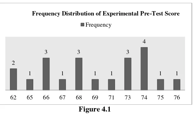
The distribution of students’ pre-test score can also be seen in the following figure.
Figure 4.1
Histogram of Frequency Distribution of Experimental Pre-Test Score
2
1 3
1 3
1 1 3
4
1 1
62 65 66 67 68 69 71 73 74 75 76
Frequency Distribution of Experimental Pre-Test Score
Frequency
It can be seen from the figure above, the students’ pretest score in experimental class. There were two students who got score 62. There was one student who got score 65. There were three students who got score 66. There was one student who got score 67. There were three students who got score 68. There was one student who got score 69. There was one student who got score 71. There were three students who got score 73. There were four students who got score 74. There was one student who got score 75 and there was one student who got score 76.
The next step, the result calculated the scores of mean, standard deviation, and standard error using SPSS 18 program and manual calculation as follows:
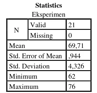
Table 4.1 the Calculation of Mean, SD and SE using SPSS 18 Statistics
Eksperimen
N Valid 21
Missing 0
Mean 69,71
Std. Error of Mean ,944 Std. Deviation 4,326
Minimum 62
Maximum 76
Based on the data above, it was known the highest score was 76 and the lowest score was 62. For the result of manual calculation, it was found that the mean score of pre-test was 69,71, the standard deviation was 4,222 and for the standard error was 0,944 (see appendix).
standard deviation 4,326 and the standard error of mean of the pre-test score was 0,944.
b. The result of Pre-test Score of Control Class
The students’ pre-test score of control class were distributed in the following table (see appendix) in order to analyze the students’
knowledge before post-test. To determine the frequency of score, percent of score, valid percent and cumulative percent calculated using SPSS 18 (see appendix).
The distribution of students’ pre-test score can also be seen in the following figure.
Figure 4.2
Histogram Frequency Distribution of Control Pre-Test Score
It can be seen from the figure above, the students’ pre-test score in control class. There were two students who got score 62. There were five students who got score 65. There were six students who got score 67. There were four students who got score 68. There was one student who got score 69. There were two students who got score 71. There was one student who got score 75.
0 1 2 3 4 5 6 7
62 65 67 68 69 71 75
Frequency Distribution of Control Pre-Test Score
The next step, the result calculated the scores of mean, standard deviation, and standard error using SPSS 18 program and manual calculation as follows:
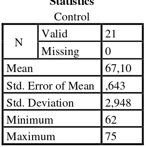
Table 4.2 the Calculation of Mean, SD and SE using SPSS 18
Statistics Control
N Valid 21
Missing 0
Mean 67,10
Std. Error of Mean ,643 Std. Deviation 2,948
Minimum 62
Maximum 75
Based on the data above, it was known the lowest score was 62 and the highest score was 75. For the result of manual calculation, it was found that the mean score of pre-test was 67,09, the standard deviation was 2,877 and for the standard error was 0,643 (see appendix).
Based on the table above, the result calculation using SPSS 18, it was found that the mean of score pre-test was 67,10, the standard deviation 2,948 and the standard error of mean of the pre-test score was 0,643.
c. Testing Normality and Homogeneity using SPSS 18 1) Testing of Data Normality
Because of that, the normality test used SPSS 18 to measure the normality of the data.
Table 4.3 Test of Normality Distribution Test on the
Pre-Test Score of the Experiment and Control Group Using SPSS 18 Tests of Normality
Kelompok Kolmogorov-Smirnov
a
Shapiro-Wilk Statistic df Sig. Statistic df Sig. Nilai Experiment ,205 21 ,022 ,920 21 ,085
Control ,189 21 ,049 ,921 21 ,093
Description:
If respondent > 50 used Kolmogorov-Sminornov If respondent < 50 used Saphiro-Wilk
The criteria of the normality test pre-test was if the value of (probability value/critical value) was higher than or equal to the level of significance alpha defined (r > a), it meant that the distribution was normal. Based on the calculation using SPSS 18 above, the value of (probably value/critical value) from pre-test of the experiment and control class in Saphiro-Wilk table was higher than level of significance alpha used or r = 0,085 > 0,05 (Experiment) and r = 0,093 > 0,05 (Control). So, the distributions were normal. It meant the students’ score of pre-test had normal distribution.
2) Testing of Data Homogeneity
Table 4.4 Homogeneity Test Test of Homogeneity of Variances
Levene Statistic df1 df2 Sig.
The criteria of the homogeneity pre-test was if the value of (probability value/critical value) was higher than or equal to the level significance alpha defined (r > a), it meant the distribution was homogeneity. Based on the calculation using SPSS 18 program above, the value of (probably value/critical value) from pre-test of experiment and control class on homogeneity of variance in sig column was known that p-value was 0,178. The data in this study fulfilled homogeneity since the p-value was higher or r = 0,178 > 0,05.
2. The Result of Post-test Score
a. The Result of Post-test of Experiment Class
The students’ post-test score of experiment class were distributed in the following table (see appendix) in order to analyze the students’ knowledge after conducting the treatment. To determine the frequency of score, percent of score, valid percent and cumulative percent calculated using SPSS 18 (see appendix).
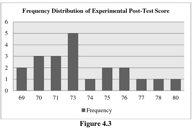
Figure 4.3
Histogram of Frequency Distribution of Experimental Post-Test Score It can be seen from the figure above, the students’ post-test score in experimental class. There were two students who got score 69. There were three students who got score 70. There were three students who got score 71. There were five students who got score 73. There was one student who got score 74. There were two students who got score 75. There were two students who got score 76. There was one student who got score 77. There was one student who got score 78 and there was one student who got score was 80.
The next step, the result calculated the scores of mean, standard deviation, and standard error using SPSS 18 program and manual calculation as follows:
0 1 2 3 4 5 6
69 70 71 73 74 75 76 77 78 80
Frequency Distribution of Experimental Post-Test Score
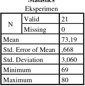
Table 4.5 the Calculation of Mean, SD and SE using SPSS 18
Statistics Eksperimen
N Valid 21
Missing 0
Mean 73,19
Std. Error of Mean ,668 Std. Deviation 3,060
Minimum 69
Maximum 80
Based on the data above, it was known the lowest score was 69 and the highest score was 80. For the result of manual calculation, it was found that the mean score of post-test was 73,19, the standard deviation was 2,987 and for the standard error was 0,668 (see appendix).
Then, based on the table above, the result calculation using SPSS 18, it was found that the mean of score post-test of the experiment class was 73,19, the standard deviation 3,060 and the standard error of mean of the post-test score was 0,668.
b. The result of Post-test Score of Control Class
The students’ post-test score of control class were distributed in the following table (see appendix) in order to analyze the students’
knowledge after pre-test. To determine the frequency of score, percent of score, valid percent and cumulative percent calculated using SPSS 18 (see appendix).
Figure 4.4
Histogram of Frequency Distribution of Control Post-Test Score It can be seen from the figure above, the students’ pos-test score in control class. There was one student who got score 64. There were five students who got score 68. There were eight students who got score 70. There were three students who got score 72. There was one student who got score 73. There was one student who got score 74. There was one student who got score 76 and there was one students who got score 78.
Next step, the result calculated the scores of mean, standard deviation, and standard error using SPSS 18 program and manual calculation as follows:
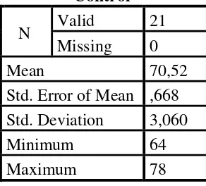
Table 4.6 the Calculation of Mean, SD and SE using SPSS 18 Control
N Valid 21
Missing 0
Mean 70,52
Std. Error of Mean ,668 Std. Deviation 3,060
Minimum 64
Maximum 78
1
5
8
3
1 1 1 1
64 68 70 72 73 74 76 78
Frequency Distribution of Control Class
Based on the data above, it was known the lowest score was 64 and the highest score was 78. For the result of manual calculation, it was found that the mean score of post-test was 70,52, the standard deviation was 2,987 and for the standard error was 0,668 (see appendix).
Based on the table above, the result calculation using SPSS 18, it was found that the mean of score post-test was 70,52, the standard deviation 3,060 and the standard error of mean of the post-test score was 0,668.
c. Testing Normality and Homogeneity using SPSS 18 1) Testing of Data Normality
It was used to know the normality of the data that was going to be analyzed whether both groups have normal distribution or not. Because of that, the normality test used SPSS 21 to measure the normality of the data.
Table 4.7 Test of Normality distribution test of
Post-Test score of the Experiment and Control group using SPSS 18 Tests of Normality
Kelompok Kolmogorov-Smirnov
a
Shapiro-Wilk Statistic df Sig. Statistic df Sig. Nilai Experiment ,144 21 ,200* ,948 21 ,313
Control ,189 21 ,049 ,921 21 ,093
Description:
The criteria of the normality test post-test was if the value of (probability value/critical value) was higher than or equal to the level of significance alpha defined (r > a), it meant that the distribution was normal. Based on the calculation using SPSS 18 above, the value of (probably value/critical value) from post-test of the experiment and control class in Saphiro-Wilk table was higher than level of significance alpha used or r = 0,313 > 0,05 (Experiment) and r = 0,093 > 0,05 (Control). So, the distributions were normal. It meant that the students’ score of post-test had normal distribution.
2) Testing of Data Homogeneity
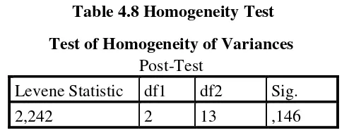
Table 4.8 Homogeneity Test Test of Homogeneity of Variances
Post-Test
Levene Statistic df1 df2 Sig.
2,242 2 13 ,146
fulfilled homogeneity since the p-value was higher or r = 0,146 > 0,05.
B. Result of Data Analysis
1. Testing Hypothesis using ttest Manual Calculation
The level of significance used 5%. It meant that the level of significance of the refusal null hypothesis in 5%. The level of significance decided at 5% due to the hypothesis type stated on non-directional (two-tailed test). It meant that the hypothesis cannot directly the prediction of alternative hypothesis. To test the hypothesis of the study used t-test statistical calculation. First, it calculated the standard deviation and the standard error of X1 and X2. It was found the standard deviation and the standard error of post-test of X1 and X2 at the previous data presentation. It could be seen in this following table:
Table 4.9 the standard Deviation and Standard Error of X1 and X2
Variable The Standard Deviation The Standard Error
X1 2,987 0,668
X2 2,987 0,668
Where:
X1: Experiment X2: Control
The next step, the result calculated the standard error of the differences mean between X1 and X2 as follows:
Standard error of mean of score between Variable I and Variable II
SEM1– SEM2 = √( ) ( )
SEM1– SEM2 = √( ) ( )
SEM1– SEM2 = √
SEM1– SEM2 = √
SEM1– SEM2 = 0,9447
SEM1– SEM2 = 0,945
The calculation above showed the standard error of the difference mean between X1 and X2 was 2,129. Then, it inserted to the formula to get the value of tobserved as follows:
To =
To =
To =
To = 2,84043
To = 2,84
Which the criteria:
If t-test (t-observed) ≥ t-table, Ha was accepted and H0 was rejected
Then, the degree of freedom (df) accounted with the formula: Df = ( )
= (21+21) – 2 = 40
The significant levels choose at 5%, it meant the significant level of refusal of null hypothesis at 5%. The significance level decided at 5% to the hypothesis stated on non-directional (two-tailed test). It meant that the hypothesis cannot direct the prediction of alternative hypothesis. The calculation above showed the result of ttest calculation as
in the table follows:
Table 4.10 the Result of ttest Manual Calculation
Variable Tobserved Ttable Df/db
5% 1%
X1-X2 2,84 2,02 2,71 40
Where:
X1 : Experiment Class X2 : Control Class
Tobserved : The calculated Value
Ttable : The Distribution of t value
Df/db : Degree of freedom
Based on the result of hypothesis test calculation, it was found that the value of tobserved was greater than the value of ttable at the level
significance in 5% or tobserved > ttable (2,84 > 2,02). It meant Ha was
It could be interpreted based on the result of calculation that Ha
stating that there was significant effect of using questioning strategy in prewriting technique toward the students’ ability in writing narrative text at the tenth grade of SMA Muhammadiyah 1 Palangka Raya was accepted and H0 stating that there was no significant effect of using
questioning strategy in prewriting technique toward the students’ ability in writing narrative text at the tenth grade of SMA Muhammadiyah 1 Palangka Raya was rejected. It meant that teaching writing using questioning strategy gave significant effect toward students’ writing ability.
2. Testing Hypothesis Using SPSS 18 Program
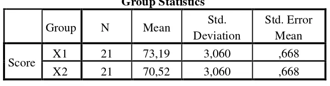
The result of the t-test using SPSS 18 program was used to support the manual calculation of the t-test. It could be seen as follows: Table 4.11 the Standard Deviation and the Standard Error of
X1 and X2 using SPSS 18 Group Statistics
Group N Mean Std.
Deviation
Std. Error Mean
Score X1 21 73,19 3,060 ,668
X2 21 70,52 3,060 ,668
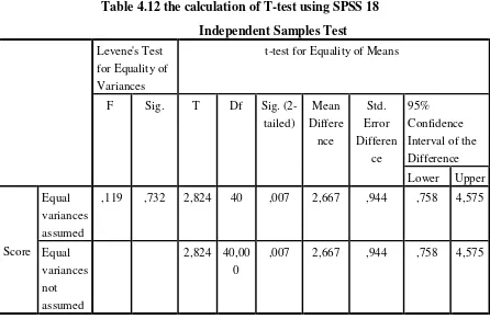
Table 4.12 the calculation of T-test using SPSS 18 Independent Samples Test Levene's Test
for Equality of Variances
t-test for Equality of Means
F Sig. T Df Sig.
(2-tailed) Mean Differe nce Std. Error Differen ce 95% Confidence Interval of the Difference
Lower Upper
Score
Equal variances assumed
,119 ,732 2,824 40 ,007 2,667 ,944 ,758 4,575
Equal variances not assumed
2,824 40,00 0
,007 2,667 ,944 ,758 4,575
The table showed the result of t-test calculation using SPSS 18 program. Since the result of post-test between experiment and control group had difference score levene’s test for equality of variance, the value of sig was greater than 0,05. So, both of group were homogeny. It meant the t-test calculation used at the equal variance assumed. It found that the value of sig (two-tailed) was 0,007 and the result of tobserved was
2,824. The result of mean difference between experimental and control class was 2,667 and the standard error difference between experimental and control class was 0,944.
3. Interpretation
sig (two-tailed) was lower than 0,05 or 0,007 < 0,05, so Ha was accepted
and H0 was rejected. The result of t-test was interpreted on the result of
degree freedom to get the ttable. The result of the degree of freedom (df)
was 40, it found from total number of the students in both group minus 2. The following table was the result of tobserved and ttable from df at 5% level.
Table 4.13 the Result ttest using SPSS 18
Variable Tobserved Ttable Df/db
5% 1%
X1-X2 2,824 2,02 2,71 40
The result of the ttest used SPSS 18 program. It was found the t
observed was greater than the t table at 5% significance level or 2,824 > 2,02. It means that Ha is accepted and H0 is rejected. The value of mean
of the experiment class (print out group descriptive) was 73,19 higher than the value of mean of the control class 70,52. So, score of experiment was greater than score of control class.
It could be interpreted based on the result of calculation that Ha
there is significant effect of questioning strategy in prewriting technique toward the students’ ability in writing narrative text at the tenth grade of SMA Muhammadiyah 1 Palangka Raya and H0 stating that there is no
C. Discussion
The result of the data analysis showes that the Questioning Strategy you gave very significance effect on the students’ writing skill for the tenth-grade students at SMA Muhammadiyah1 Palangka Raya. The students who were taught using Questioning Strategy got higher score than students who were taught without using Questioning Strategy. It was proved by the mean score of the students who were taught using Questioning Strategy was 73,19 and the students who were taught without using Questioning Strategy was 70,52. Based on the result of hypothesis test calculation, it was found that the value of Tobserved
was greater than the value of Ttable at 5% significance level or 2,84< 2,02. It
meant Ha was accepted and Ho was rejected.
Furthermore, the result of t test calculation using SPSS 18 found that the Questioning Strategy gives significance effect on the students’ Enflish score. It proved by the value df Tobserved was greater than Ttable at 5% significance level
or 2,824<2,02. The result of t-test by using SPSS and manual calculation showed that there was effect of Questioning Strategy on writing ability, it meant Questioning Strategy effective to use in the class.
Based on the results finding of the study, it is shown that Questioning Strategy gave contribution in the students’ writing skill during the instructional process. Questioning Strategy implemented in this study consists of some steps. Those are; The first meeting, explaining questioning strategy. The second meeting, the author gave an example of how to used questioning strategy to enable students to easily understand the intent of the strategy questioning. Last, the author with students working on an assignment sheet or exercise together, before I ask the students do the work.
There are some possible reasons why Questioning Strategy is effective in teaching writing at the tenth-grade students of SMA Muhammadiyah1 Palangka Raya. The first reason is when the writer taught English using Questioning Strategy gave the students’ interest and curiosity concerning a topic. The second reason is when the writer taught English using Questioning Strategy gave their focus attention on a particular issue or concept. The third reason was when the writer taught English using Questioning Strategy gave their development an active approach to learning. The last reason is when the writer taught English using Questioning Strategy communicate to the group that involvement in the lesson was expected, and that overt participation by all members of the group was valued, made students could comprehend the material easier.