Dynamic Modeling and Noncollocated Control of a Flexible Planar Cable-Driven Manipulator

Dynamic Modeling and Noncollocated Control

of a Flexible Planar Cable-Driven Manipulator

Ryan James Caverly

, Student Member, IEEE

, and James Richard Forbes

, Member, IEEE

Abstract—This paper investigates the dynamic modeling and passivity-based control of a planar cable-actuated system. This system is modeled using a lumped-mass method that explicitly considers the change in cable stiffness and winch inertia that oc-curs when the cables are wound around their respective winches. In order to simplify the modeling process, each cable is modeled in-dividually and then constrained to the other cables. Exploiting the fact that the payload is much more massive than the cables allows the definition of a modified output called theµ-tip rate. Coupling theµ-tip rate with a modified input realizes the definition of a pas-sive input–output map. The two degrees of freedom of the system are controlled by four winches. This overactuation is simplified by employing a set of load-sharing parameters that effectively re-duce four inputs to two. The performance and robustness of the controllers are evaluated in the simulation.

Index Terms—Cable-actuated systems, dynamics, motion con-trol, parallel robots, passivity-based control.

I. INTRODUCTION

T

HE use of cable-actuated systems is widespread; elevators, towing systems, cranes, aerostats, and cable robots are ex-amples of systems actuated by cables. Cable-actuated systems typically feature stationary actuating winches, which reduces the moving mass of the system compared with standard serial (rigid-link) manipulators whose actuators are embedded in the manipulator, allowing for higher payload accelerations. Cable-actuated systems also allow for relatively large workspaces and high maximum payload to weight ratios. Unfortunately, these advantages can be overshadowed by the fact that the cables used in these systems are relatively flexible and only provide an actuating force in tension, not in compression. These short-comings are often addressed by reducing the acceleration of the desired trajectory, so that cable vibrations are not excited, or using shorter cables [1]. Although this may solve the issue of cable vibration, the performance capability of cable-actuated systems is not fully exploited.

Cable-actuated systems differ from rigid manipulators by the flexibility present in the cables. In cable robot applications, this flexibility is often ignored and the cables are assumed to be straight and massless [1]–[5]. For systems with relatively short

Manuscript received January 14, 2014; revised May 16, 2014; accepted Au-gust 8, 2014. Date of publication September 4, 2014; date of current version December 3, 2014. This paper was recommended for publication by Associate Editor P. R. Giordano and Editor T. Murphey upon evaluation of the reviewers’ comments.

The authors are with the Department of Aerospace Engineering, Univer-sity of Michigan, Ann Arbor, MI 48109 USA (e-mail: caverly@umich.edu; forbesrj@umich.edu).

Color versions of one or more of the figures in this paper are available online at http://ieeexplore.ieee.org.

Digital Object Identifier 10.1109/TRO.2014.2347573

cables, this may be a valid assumption, which simplifies the dynamic model of the system, as well as any controller synthesis. Unfortunately, in large-scale cable-actuated systems, such as cable-tethered aerostats [6], this flexibility cannot be ignored. The dynamic modeling of cable-actuated systems considering cable flexibility has been developed in [7]–[10], using variations of a lumped-mass method. This modeling method lumps the mass of the continuous cable into discrete locations and models the cable flexibility and natural damping by placing springs and dampers between the lumped masses.

The flexibility associated with cables leads to the issue of noncollocation. The goal of cable-actuated systems is to control the position and velocity of a payload located at the opposite end of many flexible cables actuated by winches. Due to this noncollocation, a passive map cannot be established from the in-put torque of the winches to the outin-put velocity of the payload, and hence, passivity-based control techniques are not readily applicable. When controlling flexible robotic manipulators, the use of a modified input and a modified output was shown to provide a passive input–output map in [10]–[18]. In particular, in [14]–[18], theµ-tip rate, which scales the effect of the elastic coordinates when calculating the payload velocity, is defined. Theµ-tip rate was implemented on a single-degree-of-freedom (DOF) cable-actuated system in [10], proving that multiple pas-sive mappings can be established.

This paper extends the study presented in [10] by deriving the nonlinear dynamic model of a planar cable-actuated system and implementing passivity-based control on the planar system. This is accomplished by first fully developing the lumped-mass model of a single cable and constraining two of these cables together to create a two-cable system. Two of these two-cable systems are then constrained together to capture the dynamics of the complete planar system, which consists of four cables and one payload moving in the plane. The mass and stiffness param-eters of the cable change as the cable is wound in or let out. The rigid and elastic dynamics of the complete system are then ap-proximately decoupled by making the assumption of a massive payload [14]. This, along with the definition of theµ-tip rate, allows the establishment of various passive input–output maps. Passivity-based control is then implemented in the simulation, which illustrates the system’s performance. The novel contri-bution of this study is the development of the dynamic model using a Lagrangian-based lumped-mass method, the establish-ment of multiple passive mappings, and the proof of closed-loop stability of a planar cable-actuated system. The dynamic model of the planar cable-actuated system is presented with a large amount of detail in an effort to avoid any ambiguity in the derivation.

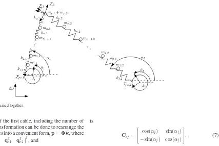
Fig. 1. (a) Schematic of a planar cable-actuated system with four cables and (b) lumped-mass model of a single cable.

II. PRELIMINARIES

A. Passive Systems

The mappingu→yassociated with the operatorG:L2e → L2e, wherey=Gu, is input strictly passive (ISP) if∃β and 0< δ <∞, such that [19]

T

0

yT(t)u(t)dt≥δu22T +β, ∀u∈L2e, T∈R+.

When δ= 0, the mapping is passive. The weak form of the Passivity Theorem states that a passive system connected in a negative feedback loop with an ISP system isL2stable [19].

B. Lagrangian Dynamics

The equations of motion of a rigid body can be found by solving Lagrange’s equation

d dt

_∂L

∂q˙

T −

_∂L

∂q

T

+

_∂R

∂q˙

T

=f+ΞTλ ₍₁₎

whereL=T−V is the Lagrangian,R is the Rayleigh dissi-pation function,q are the generalized coordinates, f are the generalized forces, Ξ is the Jacobian matrix associated with the system’s constraints, andλ_{are the Lagrange multipliers. A} transpose is applied to each term on the left-hand side of (1) to keep the equation consistent with the definition of a Jacobian [20].

III. SYSTEMDYNAMICS

Consider the planar cable-actuated system shown in Fig. 1(a). It is characterized by a payload of mass4mp, four cables, and

four actuating winches. At least three cables are required to provide two DOFs, because of the unidirectional capability of cables. In this paper, four cables will be used, realizing a larger workspace and making for a more intuitive derivation of the system’s dynamics.

In this section, the lumped-mass dynamic model of each ca-ble is derived individually and, then, constrained together. The lumped-mass method used derives from [7]–[10], [21], and [22]. As in [22], the dynamics of the winches are considered, which takes into account the additional inertia added to the winches because of the wrapping of the cable. In systems with very large cables, this additional winch inertia can be significant. The assumptions made in the following derivation of the dy-namic model include that the payload moves in the plane, the tensions in the cables are large enough that gravitational forces on the cable lumped masses can be neglected, and the mass of the payload is much greater than the mass of the cables, which allows for an approximate decoupling of the dynamics in Section III-D. Further assumptions could be made to simplify the dynamic model, but it was decided to maintain a certain amount of fidelity in the model. For instance, many dynamic models [2], [7] do not include winch dynamics, which simpli-fies the model. In practice, a winch is needed to wind the cable, and as such, a realistic and practical dynamic model should include this effect. In addition, the passive maps presented in this paper rely on the fact that the energy of the undamped and unforced system is constant, which would not be true if mass were added and removed representing cable lengthening and shortening. For this reason, the modeling of winch dynamics and cable wrap is of great use.

A. Modeling a Single-Cable System

A schematic of a single winch-driven cable modeled withn lumped masses attached to a payload is shown in Fig. 1(b). Let

Fi,Fw ,1, andF1 denote the inertial frame, the frame attached

to the first winch, and the frame attached to the first cable, respectively. TheFw ,1frame is located at the center of the first

winch, and theF1 frame is located at the payload.

The kinetic energy, T1, potential energy, V1, and Rayleigh

dissipation function, R1, of the single-cable system are

T1 = 1₂q˙T1M1q˙1, V1 = 1₂qT1K1q1, and R1 =₂1q˙T1D1q˙1,

re-spectively, where q1 = [θ1 qTe1 α1]T are the

general-ized coordinates of the first cable, θ1 is the rigid

coor-dinate representing the rotation of the winch drum, qe1 =

[x1,1 x2,1 . . . xn ,1 xp,1]T are the relative flexible

co-ordinates of the cable,α1is the angle of rotation between frame

Fi and F1, M1 =MT1 =Mp,1+Mw ,1+ni= 1Mi,1 >

0is the mass matrix,K1 =KT1 =diag{0, k1,1, k2,1, . . . , kn ,1,

kp,1,0} ≥0 is the stiffness matrix, D1 =DT1 =diag{0,

c1,1, c2,1, . . . , cn ,1, cp,1,0} ≥0is the damping matrix, and

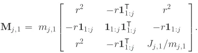
Mp,1 = mp,1

⎡

⎢ ⎢ ⎣

r2 _−r1T

1:n+ 1 r2

−r11:n+ 1 11:n+ 11T1:n+ 1 −r11:n+ 1

r2 _−r1T

1:n+ 1 Jp,1/mp,1

⎤

⎥ ⎥ ⎦

Mw ,1 =

J1 0

0 0

Mj,1 = mj,1 1 0]T_{is a column vector composed of ones starting at indexi}

and ending at indexj, with every other entry zero.

The mass of each lumped mass is calculated as m1,1 =

σA(L1/n−rθ1)andmi,1 =σAL1/n, i=2,3, . . . , n, where

A is the cross-sectional area of the cable, L1 is the nominal

length of the cable,σ is the density of the cable, andr is the radius of the winch. The first lumped mass changes its value as the cable is wrapped around the winch drum, decreasing the total mass of the cable. The stiffness of each cable seg-ment is calculated as k1,1 =EA/(L1/(n+ 1)−rθ1),ki,1 =

EA(n+ 1)/L1, i=2,3, . . . , n, and kp,1=EA(n+ 1)/L1,

whereEis the modulus of elasticity of the cable. The longitu-dinal stiffness of each cable is clearly a function of the cable’s length, which is why the stiffness of the first cable segment changes as the cable is wrapped around the winch drum. The second moment of mass of the winch about the winch’s axis of rotation isJ1 =Jw ,1+σAr3θ1, whereJw ,1 is the nominal

second moment of mass of the winch, andσAr3_θ

1 is an

ad-ditional second moment of mass term resulting from the cable winding around the winch. The second moment of mass of each lumped mass about the i

→3axis isJj,1 =mj,1(r

perpendicular to the plane of motion. Similarly, the second moment of mass of the payload mass about the i

→3 axis is

Jp,1 =mp,1(r2+ (L1+j_{k= 1}xk ,1+xp,1−θ1r)2).

Using a Lagrangian formulation, the equations of motion of the single-cable system are

These terms account for the nonlinear effects because of the changing mass and stiffness of the first cable segment, where∂/˜ ∂q˜ 1(1₂q˙T1M1q˙1) = ˜∂/∂q˜ 1(1₂q˙T1Mp,1q˙1) +

˜

∂/∂˜q1(1₂q˙1TMw ,1q˙1) +nj= 1∂/˜ ∂˜q1(1₂q˙T1Mj,1q˙1)is the

par-tial derivative of the kinetic energy with respect to q1, while

keeping the termsq˙T

1 andq˙1 constant, and∂/˜ ∂˜q1(1₂qT1K1q1)

is the partial derivative of the potential energy with respect to q1, while keeping the termsqT1 andq1 constant. The nonlinear

terms are given by

above are significantly more complicated than the ones presented in [10] because of the additional DOF.

B. Modeling a Two-Cable System

The null-space method [23] will be employed to constrain two single cables together to form a two-cable system. If cables could operate in tension and compression, two cables would be sufficient to fully actuate the system in two DOFs. Due to the unidirectionality of cables, the two-cable system, shown in Fig. 2, does not provide two DOFs. The dynamic model of the two-cable system will be developed as a stepping stone toward the complete system.

Before constraining two cables together, the equations of mo-tion of the two cables must be expressed in a convenient form. The generalized coordinates of the two-cable system are writ-ten asp=

θ1 qTe1 α1 θ2 qTe2 α2T. The unconstrained

equations of motion of the complete system are

Mpp¨+Dpp˙ +Kpp=Bpτ +fnon,p (3)

Fig. 2. Two cables constrained together.

different from those of the first cable, including the number of lumped masses. A transformation can be done to rearrange the generalized coordinates into a convenient form,p˙ =Φκ˙, where κ= [θ1 θ2 α1 α2 qTe1 qTe2]

T

, and

Φ=

⎡

⎢ ⎢ ⎢ ⎢ ⎢ ⎢ ⎣

1 0 0 0 0 0

0 0 0 0 1 0

0 0 1 0 0 0 0 1 0 0 0 0

0 0 0 0 0 1

0 0 0 1 0 0

⎤

⎥ ⎥ ⎥ ⎥ ⎥ ⎥ ⎦

.

This allows the rigid coordinates to be assembled together and the elastic coordinates to be assembled together. Applyingp˙ = Φκ˙ and premultiplying (3) byΦTgives

Mκκ¨+Dκκ˙ +Kκκ=Bκτ+fnon,κ (4)

where Mκ =ΦTMpΦ, Dκ =ΦTDpΦ, Kκ =ΦTKpΦ, Bκ =ΦTBp, andfnon,κ=ΦTfnon,p. The payload velocity can

be described by either the generalized coordinates of the first cable system or the second cable system

˙

ρ= Jθ1θ˙1+Je1q˙e1+Jα1α˙1 (5)

= Jθ2θ˙2+Je2q˙e2+Jα2α˙2 (6)

where Jθ1 =Ci1[−r 0 ]T and Jθ2 =Ci2[−r 0 ]T are the

rigid Jacobians of the first and second cable systems, respec-tively; Je1 =Ci1[11:n+ 1 0]T and Je2 =Ci2[11:n+ 1 0]T

are the elastic Jacobians of the first- and second-cable systems, respectively; and Jα1 =Ci1[−r L1+n_{k= 1}xk ,1+xp,1−

θ1r]T and Jα2 =Ci2[−r L2+nk= 1xk ,2+xp,2−θ2r]T

are the Jacobians associated with the angleαfor the first and second cable systems, respectively. The matricesCi1 andCi2

are rotation matrices that describe the rotation fromF1 toFi

and the rotation fromF2 toFi, respectively, whereFj defines

reference framej. The rotation matrix fromFj toFi,Cij(αj),

is

Cij =

cos(αj) sin(αj)

−sin(αj) cos(αj)

. (7)

The two cables can be constrained together by forcing the pay-load velocity described by both to be identical. Equating (5) and (6) and isolating forα˙1andα˙2 gives

˙ α1

˙ α2

= ˆJ−_α1(Jθ2θ˙2+Je2q˙e2 −Jθ1θ˙1−Je1q˙e1) =Qq˙12

(8) where Jˆα =Jα1 −Jα2, and Q= ˆJ−α1[−Jθ1Jθ2 −Je1

Je2]. Equation (8) can be used to relate the unconstrained

coordinates to the constrained coordinates, κ˙ =Γq˙12, where

q12 =θ1 θ2 qTe1 qTe2

T , and

Γ=

⎡

⎢ ⎣

1 0

Q

0 1 ⎤

⎥

⎦. (9)

Subtracting (6) from (5) gives the constraint equationΨκ˙ =0, where Ψ=

Jθ1 −Jθ2 Jα1 −Jα2 Je1 −Je2.

Premul-tiplying (4) byΓTand applying the constraints gives

ΓTMκΓ¨q12+ΓTDκΓq˙12+ΓTKκκ=ΓTBκτ

+ΓTfnon,κ−ΓTMκΓ˙κ˙ +ΓTΨTλ(10)

whereλ_{are the Lagrange multipliers associated with the} con-straints. This can be restated as

M12q¨12+D12q˙12+K12q12 =B12τ+fnon,12 (11)

where M12 =ΓTMκΓ, D12 =ΓTDκΓ, K12q12 =ΓTKκκ, B12=ΓTBκ, and fnon,12 =ΓT(fnon,κ−MκΓ˙κ˙).

Substitut-ing κ˙ =Γq˙12 into Ψκ˙ =0 gives the result ΓTΨTλ=0 by

The payload velocity can be fully described by

˙

ρ=Jθ12θ˙12+Je12q˙e12 (12)

whereθ˙12 = [θ1 θ2]T,q˙e12 = [ ˙qTe1 q˙Te2]

T

, and

Jθ12(θ12,qe12) = [Jθ1 0] + [Jα1 0]ˆJ−α1[−Jθ1 Jθ2]

Je12(θ12,qe12) = [Je1 0] + [Jα1 0]ˆJ−α1[−Je1 Je2].

Note that the Jacobians of the single-DOF two-cable system [10] are constant, and in particular, the rigid Jacobians are scalar val-ues. In this paper, the Jacobians are clearly functions of θ12

andqe12, and the rigid Jacobian is a matrix. This adds an

ad-ditional degree of complexity to the dynamic model and the control formulation in Section IV. In practice, the rigid and elastic Jacobians of the two-cable system are approximated as Jθ12(θ12,qe12)≡Jθ12(θ12,0) and Je12(θ12,qe12)≡

Je12(θ12,0)[15].

See the Appendix for an explicit derivation of the equations of motion for a two-cable system with a single lumped mass in each cable.

C. Modeling the Complete System

A similar process to that described in the previous section is used to derive the equations of motion of the complete four-cable system. Before constraining two of the two-four-cable sys-tems together to obtain the complete system, the equations of motion of both two-cable systems will be expressed to-gether. The generalized coordinates of the complete system areq= [θT12 qTe12 θT34 qTe34]

T

. After assembly, the uncon-strained equations of motion of the complete system are

Mq¨+Dq˙ +Kq= ˆBτ+fnon (13)

where M=diag{M12,M34}, D=diag{D12,D34}, K=

diag{K12,K34}, fnon = [fnonT ,12 fnonT ,34]

T

, Bˆ =diag{B12,

B34}, andτ = [τT12 τT34]

T

. Note that the subscript34denotes the properties of a second two-cable system. The equations of motion of the second two-cable system are identical to the first, with the values of the second system substituted in. A transfor-mation can be done to rearrange the generalized coordinates,

˙

q=Υη˙, whereη= [θT12 θT34 qTe12 qTe34]

T

, and

Υ=

⎡

⎢ ⎢ ⎣

1 0 0 0

0 0 1 0

0 1 0 0

0 0 0 1

⎤

⎥ ⎥ ⎦

.

Applyingq˙ =Υη˙ and premultiplying (13) byΥTgives ¯

M¨η+ ¯Dη˙ + ¯Kη= ¯Bτ+ ¯fnon (14)

whereM¯ =ΥTMΥ,D¯ =ΥTDΥ,K¯ =ΥTKΥ,B¯ =ΥTBˆ, and¯fnon =ΥTfnon. The parameters of the transformed

equa-tions of motion found in (14) can be partitioned as

¯

M=

Mθ θ Mθ e

Meθ Mee

¯

D= diag{0,Dee}, K¯ =diag{0,Kee}.

In order to constrain the first two-cable system to the second two-cable system, the payload velocity of both systems must be the same. To accomplish this, the null-space method will be employed [23] as was done previously for the two-cable system. The constraint can be written asΞη˙ =0where Ξ=

Jθ12 −Jθ34 Je12 −Je34. The dependent generalized

ratesη˙ can be related to the independent generalized ratesz˙by ˙

η=Rz˙where

R=

Rθ r Rθ e

Rer Ree

, z=

⎡

⎢ ⎣

θ12

qe12

qe34

⎤

⎥ ⎦.

The components ofRare

Rθ r =

1 ˆ Rθ r

, Rθ e =

0 ˆ Rθ e

, Rer =0,Ree=1

where Rˆθ r =J−θ341 Jθ12, Rˆθ e =Rˆθ e,1 Rˆθ e,2

, Rˆθ e,1 =

J−_θ341Je12, and Rˆθ e,2 =−J−θ341Je34. After premultiplying by

RT_{, this transforms (14) to}

RTMR¨¯ z+RTDR˙¯ z+RTK¯η=RTB¯τ+RT¯fnon

−RTM¯R˙˙z+RTΞTλ ₍₁₅₎ whereλ_{are the Lagrange multipliers associated with the} con-straint. The termRTΞTλ_{=0, which can be shown by} substi-tutingη˙ =Rz˙ intoΞη˙ =0. The equations of motion are now given as

Mz zz¨+Dz zz˙ +Kz zz=Bz zτ+fnon,z z (16)

where Mz z =RTMR¯ , Dz z =RTDR¯ , Kz zz=RTK¯η, Bz z =RTB¯, andfnon,z z =RT¯fnon−RTM¯R˙z˙. The reduced

mass, damping, and stiffness matrices are now in the form

Mz z =

Mz z ,r r Mz z ,r e

MT

z z ,r e Mz z ,ee

Dz z = diag{0,Dee},Kz z =diag{0,Kee}

where Mz z ,r r = RTθ rMθ θRθ r, Mz z ,r e= RTθ r[Mθ θRθ e+ Mθ e], andMz z ,ee =Mee.

The payload velocity is

˙

ρ=UT_θθ˙+UT_eq˙e (17)

where θ˙ = [ ˙θT₁₂ θ˙T₃₄]T_{, q˙}

e= [ ˙qTe12 q˙Te34]T, UTθ = [C1Jθ12

C2Jθ34], andUTe = [C1Je12 C2Je34], provided that0< C1 <

1andC2 = 1−C1. The constantsC1 andC2are load-sharing

parameters that will be discussed further in Sections III-D and IV-A.

It can be shown analytically that the energy of the com-plete system without an input torque or damping is constant for all time. The total energy of the system isH = 1

2z˙TMz zz˙ + 1

2zTKz zz. The temporal derivative of the total energy is

˙

H = ˙zT(Mz z¨z+Kz zz) + 1 2z

T_K˙ z zz+

1 2z˙

T_M˙ z zz˙

= ˙zT(fnon,z z−Dz zz˙+Bz zτ) + 1 2z

T_K˙_{z zz+}1 2z˙

T_M˙ _{z zz˙}

Without an input torque or damping, the time derivative of the total energy of the system is clearly zero.

D. Simplification Using the Massive Payload Assumption

It will be convenient in Section IV to approximately decou-ple the rigid coordinate dynamics from the elastic coordinate dynamics. To accomplish this, it will be assumed that the mass of the payload is much greater than that of the cables. As shown in [14], this assumption allows the kinetic energy of the system to be approximated by T≃Tρ+Te, where Tρ is the kinetic

energy of only the payload moving, andTe is the kinetic

en-ergy of the flexible coordinates vibrating when the payload is at rest. When the payload is moving, the kinetic energy associated with the motion of the payload will be much greater than the kinetic energy associated with the motion of the elastic coordi-nates. This allows the total kinetic energy of the system when the payload is in motion to be approximated by only the kinetic energy of the payload. When the payload is at rest, only the kinetic energy associated with the elastic coordinates is consid-ered. The total energy of the system is then approximated by the summation of bothTρ andTe.

To find the kinetic energy of the payload in motion, the ap-proximation q˙e= ¨qe ≃0is used. Substituting this into (16)

gives the payload equation of motion

Mz z ,r rθ¨12 =Jθ12τˆc+fnon,z z θ (19)

and premultiplying byJ−_θ121 gives

Mρρρ¨−fnon,ρ= ˆτc

where Mρρ=J−θ121Mz z ,r rJθ−121 , and fnon,ρ=J−θ121 fnon,z z θ+ MρρJ˙θ12θ˙12. The nonlinear term can be expressed asfnon,ρ = Cρ(ρ,ρ˙) ˙ρ+Gρ(ρ), where Cρ(ρ,ρ˙) contains the nonlinear

terms relating to the varying mass and is constructed so that 2Cρ−M˙ ρρ is skew symmetric, andGρ(ρ)contains the

non-linear terms relating to the varying stiffness. This gives the new equation of motion

Mρρ(ρ)¨ρ−Cρ(ρ,ρ˙) ˙ρ−Gρ(ρ) = ˆτc. (21)

The kinetic energy of the system at rest is found by set-tingρ˙ = ¨ρ=0. This impliesJθ12θ˙12+Je12q˙e12 =0, which

when rearranged gives θ˙12 =−Jθ−121Je12q˙e12. This can be

modified to include all elastic coordinates by defining an augmented elastic Jacobian Jˆe12=Je12 0, which now

gives θ˙12 =−J−_θ121Jˆe12q˙e. Taking the time derivative of θ˙12

gives θ¨12 =−Jθ−121 Jˆe12q¨e−( ˙J

−1

θ12Jˆe12+Jθ−121J˙ˆe12) ˙qe.

Sub-stituting this into (16) produces the equations of motion for

the elastic coordinates

ness term in (23) is found by taking the stiffness term in (22) and substituting into the form of Kz z, giving Kz zz=

0 (Keeqe)TT. After premultiplying byBTe, this simply

be-comes Keeqe, which is equivalent to Kˆeeqe. Note that the

mass and stiffness matrices are functions of the elastic co-ordinates. The nonlinear term can be expressed as fnon,e = Ce(qe,q˙e) ˙qe+Ge(qe), where

is a matrix containing the nonlinear terms related to the varying mass parameters, and

is a column vector containing the nonlinear terms relating to the variable stiffness of the system. The matrix Ce is constructed

in such a way that(2Ce−M˙ˆee)is skew symmetric. It will be

convenient to writeGe(qe)in an alternate form

Ge(qe) =

(26) is never actually computed and is only used to demon-strate the passivity of the system in Section IV-A. When us-ing (25) to calculate Ge(qe), there is no singularity in θ˙1,

in (26). Premultiplying (26) byq˙T_e gives the following:

˙

qT_eGe(qe) =−1 2q

T

eK˙ˆeeqe. (27)

coordinates can be written as

ˆ

Mee(qe)¨qe+ ˆDeeq˙e+ ˆKee(qe)qe

=−Ueτˆc+Ce(qe,q˙e) ˙qe+Ge(qe). (28)

The kinetic and potential energies of the elastic coordinates are Te= 1₂q˙TeMˆeeq˙eandVe =1₂qTeKˆeeqe. Their time derivatives,

to be used later, are

˙

Te= ˙qTeMˆeeq¨e+ 1 2q˙

T

eM˙ˆeeq˙e (29)

˙

Ve= ˙qTeKˆeeqe+ 1 2q

T

eK˙ˆeeqe. (30)

IV. CONTROLFORMULATION

As stated by the Passivity Theorem, the L2 stability of a

passive system connected to an ISP system within a negative feedback loop is assured. As such, identifying one or more pas-sive input–output maps is of significant interest. In this section, it will be shown that several passive mappings can be estab-lished for the planar cable-actuated system, which will be used in conjunction with ISP controllers to guarantee theL2stability

of the closed-loop system.

The mapping from input torque to payload velocity in a planar cable-actuated system is not necessarily passive because of the noncollocation of the system. A similar issue has been studied in flexible manipulators, leading to the use of a modified output tip rate, which has been shown to yield a passive map [11]–[18]. In particular, the reflected tip position is used in [11] and [12], an arbitrary point located inboard of the tip is used [13], and a modifiedµ-tip payload rate is used in [14]–[18].

A. µ-Tip Rate

Consider theµ-tip rate,ρ˙µ, defined as

˙

ρµ = Jθ12θ˙12+µJe12q˙e12 (31)

= µρ˙ + (1−µ)Jθ12θ˙12 (32)

= ˙ρ−(1−µ)Je12q˙e12 (33)

where 0≤µ <1 is a real number. To derive (32), add and subtractµJθ12θ˙12 from (31); to derive (33), add and subtract

Je12q˙e12 from (31). Equivalently, all terms relating to the “12”

system could be replaced by terms relating to the “34” system in the above definition. Theµ-tip rate can be interpreted as the velocity of the payload, with a weightµthat scales the influence of the time rate of change of the elastic coordinates. For specific values ofµ, physically meaningful quantities are produced. The true velocity of the payload is captured whenµ= 1, the veloc-ity of the payload as if the system were not flexible is captured when µ= 0, and the reflected velocity of the payload is cap-tured whenµ=−1. Theµ-tip rate can also be calculated using the payload velocity equation of (17):ρ˙_µ =UT_θθ˙ +µUT

eq˙e= (1−µ)UT

θθ˙ +µρ˙ = ˙ρ−(1−µ)UTeq˙e. Note that the µ-tip

rate can be found using only the rigid and elastic components of the first two-cable system, only the rigid and elastic compo-nents of the second two-cable system, or a linear combination

of both. The influence of the first and second two-cable sys-tems is determined by the load-sharing parametersC1andC2,

which are embedded in Uθ andUe, where0< C1 <1, and

C2 = 1−C1.

Theorem 1:Consider the cable-actuated system described by the equations of motion of (16). The mapτˆc→ρ˙µ is passive.

Proof.Consider the nonnegative function [14]

Hµ = H−µ(Te+Ve)

= Tρ+ (1−µ)(Te+Ve), 0≤µ <1.

Taking the time derivative ofHµ and using (18) and (27)–(30)

results in

˙

Hµ = ˙H−µ( ˙Te+ ˙Ve)

= −z˙TDz zz˙+ ˙zTBz zτ−µ

˙ qT_eKˆeeqe

+1 2q

T

eK˙ˆeeqe+ ˙qTeMˆee¨qe+ 1 2q˙

T eM˙ˆeeq˙e

= −z˙TDz zz˙+ ˙θTUθτˆc−1 2µq

T

eK˙ˆeeqe−1 2µq˙

T eM˙ˆeeq˙e

−µq˙T_e(−Dˆeeq˙e+Ceq˙e+Ge−Ueτˆc)

= ˙θTUθτˆc+µq˙TeUeτˆc−z˙TDz zz˙+µq˙TeDˆeeq˙e = ˙ρTµτˆc−z˙TDz zz˙ +µq˙TeDˆeeq˙e. (34)

Integrating (34) and knowing thatz˙T_D

z zz˙ = ˙qTeDˆeeq˙egives

T

0

˙

ρTµτˆcdt=Hµ(T)−Hµ(0) + (1−µ)

T

0

˙

zTDz zzdt.˙

(35) For0≤µ <1, (35) simplifies to

T

0

˙

ρTµτˆcdt≥ −Hµ(0)

which proves that the map fromτˆctoρ˙µis passive .

A PD control law of the form [14]τˆc=−Kpρµ+Kdρ˙µ

can now be used to stabilize the system in anL2sense.

B. µ-Tip Rate Tracking

In order to track a desired trajectory, consider the PD control law found in [14]:τˆ=−(Kpρ˜µ +Kdρ˙˜µ), whereρ˜µ =ρµ −

ρµ,d is the tracking error of theµ-tip position, andρ˙˜µ = ˙ρµ − ˙

ρµ,dis the tracking error of theµ-tip rate. The termρµ =µρ+ (1−µ)F12(θ12)is theµ-tip position, whereρis the position

of the payload andF12is the rigid forward kinematic map. The

terms ρµ,d and ρ˙µ,d correspond to the prescribed desiredµ

-tip payload position andµ-tip payload rate, respectively. Very often these terms are approximated asρ_µ,d ≃ρ_d andρ˙_µ,d ≃

˙

desired kinematics into (21) and (28)

Mρρ(ρ)¨ρd−Cρ(ρ,ρ˙) ˙ρd −Gρ(ρ) = ˆτd (36) ˆ

Mee(qe)¨qe,d+ ˆDeeq˙e,d+ ˆKee(qe)qe,d =−Ueτˆd +Ce(qe,q˙e) ˙qe,d+Ge,d(qe,qe,d,q˙e,q˙e,d) (37)

whereτˆd is the desired feedforward torque, and Ge,d(qe,qe,d,q˙e,q˙e,d)

this point onwards in the interest of brevity. The desired payload dynamics are then added to the PD control law as a feedforward component

ˆ

τc= (Mρρ(ρ)¨ρd−Cρ(ρ,ρ˙) ˙ρd−Gρ(ρ))−(Kpρ˜µ+Kdρ˙˜µ).

(39) Similar to (26), (38) does not need to be calculated online for the purposes of the feedforward control. Equation (39) clearly shows only the desired payload dynamics from (36) are used. The form ofGe,din (38) is only introduced to assist later in the

passivity analysis of the system.

It will be useful to calculate the error dynamics of the payload and the elastic coordinates, for use in the passivity analysis. This is accomplished by subtracting (36) from (21) and (37) from (28)

Mρρ(ρ)¨˜ρ−Cρ(ρ,ρ˙) ˙˜ρ= ˆτc−τˆd (40)

Additionally, it is worth noting that

˙˜

qT_eG˜e=−1 2q˜

T

eK˙ˆee˜qe. (43) Theorem 2:Consider the cable-actuated system described by the equations of motion of (16). The map(ˆτc−τˆd)→ρ˙˜µ is

passive.

Proof:Consider the nonnegative function [14]

Sµ =

Now consider an alternative form of tracking error known as the filtered error,sµ = ˙˜ρµ+Λρ˜µ, whereΛ=ΛT >0[20]. In

addition, the virtual reference trajectory and its corresponding error are defined as ρ˙r= ˙ρd −Λ˜ρµ andρ˙˜r = ˙ρ−ρ˙r = ˙˜ρ+ Λ˜ρµ[15]. Combining the definition of the virtual reference

tra-jectory and the definition of theµ-tip rate allows for an alternate representation of the filtered error:sµ = ˙˜ρr−(1−µ)UTeq˙˜e.

Now, consider the derivative control law [15]:τˆ =−Kdsµ.

Once again, the control law can be augmented with a feedfor-ward component. The desired system dynamics are found by selectively substituting in the desired kinematics into (21) and (28)

subscript d’s replaced byr’s. The virtual reference trajectory payload dynamics of (45) can be added to the derivative control law to obtain

ˆ

τc=Mρρ(ρ)¨ρr−Cρ(ρ,ρ˙) ˙ρr−Gρ(ρ)−Kdsµ. (47)

It will be useful to calculate the virtual reference trajectory error dynamics to assist in the passivity analysis of the system. The error dynamics are found by subtracting (45) from (21) and (46) from (28)

ˆ

Mee(qe)¨˜qe+ ˆDeeq˙˜e+ ˆKee(qe)˜qe

=−Ue(ˆτc−τˆr) +Ce(qe,q˙e) ˙˜qe+ ˜Ge (49)

whereq˜e =qe−qe,r,G˜eis defined by (42), and (43) remains

unchanged.

Theorem 3:Consider the cable-actuated system described by the equations of motion of (16). The map(ˆτc−τˆr)→sµ is

passive.

Proof:Consider the nonnegative function [15]

V =1 2ρ˙˜

T

rMρρρ˙˜r+ 1

2(1−µ)( ˙˜q T

eMˆeeq˙˜e+ ˜qTeKˆee˜qe) (50)

where 0≤µ <1. Taking the time derivative of V and using (43), (48), and (49) leads to

˙

V= sT_µ(ˆτc−τˆr)−(1−µ) ˙˜qTeDˆeeq˙˜e.

Integrating this relationship gives

T

0

sT_µ(ˆτc−τˆr)dt=V(T)− V(0) + (1−µ)

T

0

˙˜

qT_eDˆeeq˙˜edt

(51) For0≤µ <1, this yields

T

0

sT_µ(ˆτc−τˆr)dt≥ −V(0)

which establishes passivity from(ˆτc−τˆr)tosµ .

The results of Theorems 1–3 show that the planar cable-actuated system has three distinct passive input–output map-pings. Employing the Passivity Theorem, the closed-loop sys-tem isL2 stable as long as an ISP system is connected to the

passive system in a negative feedback loop [19]. In this section, PD and D controllers have been proposed, but in practice any ISP controller could be used to guarantee L2 stability of the

closed-loop system.

It is of interest to note that while the result of Theorem 3 cou-pled with the control law of (47) (or any ISP controller) and the Passivity Theorem guarantees that{ρ˜µ,ρ˙˜µ} ∈L2, the result of

Theorem 2 coupled with the control law of (39) (or any ISP con-troller) and the Passivity Theorem only guarantees thatρ˙˜µ ∈L2.

There is no guarantee that the tracking error will will go to zero in the case of Theorem 2. A similar attribute can be shown us-ing Theorem 1. This clearly illustrates the benefit of usus-ing the filtered error term, as it guarantees theL2 stability of both the

tracking error and the derivative of the tracking error, which is explicitly shown in the following argument. Consider the cable-actuated system described by the equations of motion of (16), with the control law of (47) and (50) as a Lyapunov function can-didateV, whereV˙ =−sT_µKdsµ −(1−µ) ˙˜qTeDˆeeq˙˜e≤0. From

Theorem 3 and the Passivity Theorem [19], it can be concluded thatsµ ∈L2. Using the definition of the filtered error guarantees

that{ρ˙˜µ,ρ˜µ} ∈L2, which in turn meansρ˜µ →0ast→ ∞. In

the interest of brevity, the proof ofρ˙˜µ →0ast→ ∞is omitted,

but a similar proof can be found in [18]. Since it has only been shown that˜ρµ →0andρ˙˜µ →0ast→ ∞and not˜ρ→0and

˙˜

ρ→0ast→ ∞, it is recommended to choose a value of µ close to1, which results inρ˜ ≃ρ˜µandρ˙˜≃ρ˙˜µ.

Although the use of theµ-tip rate as an output has many ad-vantages, there are some drawbacks and limitations to its use. For example, in order to know the values ofρµandρ˙µ,

measure-ments ofρ,ρ˙,θ12orθ34, andθ˙12orθ˙34are required, as in (32).

As a comparison, a PD control law based on the true payload position and velocity would only require a measurement ofρ andρ˙(which in practice could be accomplished using some sort of vision or camera system). As a result, in order to implement µ-tip, PD control angular encoders and tachometers would be required on at least two of the four winches. In addition, the stability results in this section rely on the assumption that the payload is massive, which in practice may not always be true. Through simulation, a minimum suitable ratio of the payload mass to the mass of the cables was found to be four or five. In cases where this assumption is not valid, a smaller value ofµ can be used. For increased performance, the choice ofµshould be made so that it is as close to1as possible, while maintain-ing stability of the closed-loop system. For added robustness to changes in the payload mass, the value ofµcan be reduced slightly.

V. NUMERICALEXAMPLE

The control laws of (39) and (47) are implemented in a dynamic simulation of the complete planar cable-actuated system. In simulation, the cable winches are lo-cated at(−0.5(m),−0.75(m)),(−0.25(m),1 (m)),(0.5(m),

−0.5(m)), and(0.4(m),0.8(m)), while the payload is initially positioned atρ0 = [−0.1 0.1]T(m). The cables have a

mod-ulus of elasticity ofE=500(MPa), a cross-sectional area of A=17.95(mm2), and a density ofσ=2200(kg/m3)and are modeled using four lumped masses. A small amount of cable damping was added with Dee=0.11. The cables are given

pretension values of 50(N), 20(N), 5.24(N), and 35.91(N)in order to maintain a positive tension in the cables at all time and to ensure that the system remains in equilibrium. The pay-load has a mass of 4mp =2(kg)and each winch has a second

moment of mass ofJ1 =1.39×10−5(kg·m2). The control

pa-rameters used wereµ=0.8, Kp =diag{6000,6000}(N/m), Kd =diag{150,150}(N/(m/s)),Λ=1(1/s),C1 =0.5, and

C2 =0.5. The desired trajectory is a spiraling circle that begins

at the initial position(−0.1,0.1), spirals out to a circle of radius 7(cm), tracks the circle for two rotations, and then spirals back in to the initial payload location. This trajectory is shown in Fig. 3(a) and is described by

ρd(t) =

⎧ ⎪ ⎪ ⎪ ⎪ ⎪ ⎪ ⎪ ⎪ ⎪ ⎪ ⎪ ⎪ ⎨

⎪ ⎪ ⎪ ⎪ ⎪ ⎪ ⎪ ⎪ ⎪ ⎪ ⎪ ⎪ ⎩

t t1

Rcosωt Rsinωt

+ρ0, 0≤t≤t1

Rcosω(t−t1)

Rsinω(t−t1)

+ρ0, t1 ≤t≤t2

t3−t

t3−t2

Rcosω(t−t2)

Rsinω(t−t2)

+ρ0, t2 ≤t≤t3

ρ0, t≥t3

whereρ0is the initial and final positions of the payload,Ris the

Fig. 3. (a) Desired trajectory and response of (b)ρyversusρxfor the circular portion of the trajectory and (c)ρ˜yversusρ˜xfor the entire trajectory.

andt1,t2, andt3are trajectory switching times. The switching

times are chosen to be multiples of the period of the circular tra-jectory, i.e.,ti =2πk/ω, i= 1,2,3,andk=1,2, . . .. The

sim-ulation uses values ofR=7(cm),ω=4π(rad/s),t1 =2.5(s),

t2 =3.5(s), and t3 =6(s). The desired trajectory is used in

(39) and (47) to calculate the feedforward control terms. In simulation, the nonlinear feedforward term, i.e.,Cρ(ρ,ρ˙) ˙ρdor Cρ(ρ,ρ˙) ˙ρr, was ignored, and the feedforward mass parameter

was perturbed to 90% of its actual value, in order to simplify the simulation and to demonstrate robustness to modeling errors. The response ofρy versusρxthroughout the circular portion of

the trajectory is given in Fig. 3(b), while the tracking errorρ˜y

versusρ˜x throughout the entire trajectory is given in Fig. 3(c).

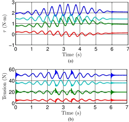
The input torquesτ1,τ2,τ3,τ4 and the cable tensionsT1,T2,

T3, andT4are presented in Fig. 4.

The results show that the payload follows the desired tra-jectory, even when faced with a significant feedforward model perturbation. The tracking errors shown in Fig. 3(c) are similar for both control laws and are less than a couple of millimeters. The root-mean-square (RMS) tracking error of the PD µ-tip controller is 1.91 (mm), and the RMS tracking error of the derivative control filtered error is 2.02 (mm). It is interesting to note in Fig. 4(a) the torque applied to the first winchτ1becomes

negative toward the middle of the trajectory, but Fig. 4(b) clearly shows that the tension remains positive in all cables. A similar phenomenon is observed using the filtered error in Fig. 5. This occurs when the torque applied by the other winches is suffi-cient for the torque applied to winch 1 to be negative, while maintaining positive cable tension.

VI. CONCLUDINGREMARKS

The dynamic model of a planar cable-actuated system has been derived using a lumped-mass method, which includes the

Fig. 4. Simulation results using theµ-tip PD controller of (a)τ1 [blue, ap-proximately centered about 2 (N·m)],τ2[green, about 0.8 (N·m)],τ3[red, about 0.2 (N·m)], andτ4[cyan, about 1.45 (N·m)] versus time. (b)T1[blue, about 50 (N)],T2 [green, about 20 (N)],T3 [red, about 5 (N)], andT4 [cyan, about 36 (N)] versus time.

Fig. 5. Simulation results using theµ-tip PD controller of (a)τ1 [blue, ap-proximately centered about 2 (N·m)],τ2[green, about 0.8 (N·m)],τ3[red, about 0.2 (N·m)], andτ4[cyan, about 1.45 (N·m)] versus time. (b)T1[blue, about 50 (N)],T2 [green, about 20 (N)],T3 [red, about 5 (N)], andT4 [cyan, about 36 (N)] versus time.

effects of longitudinal cable vibration and the modeling of winch dynamics. The modeling process begins with the modeling of a single cable and constraining the system in steps using the null-space method to derive the model of the complete system. The novel contribution of the dynamic model presented in this paper is the Lagrangian derivation of a lumped-mass cable model in two dimensions, and the use of the null-space method to derive the dynamics of a planar cable-actuated system.

theL2 stability of the closed-loop system, contributing to the

novelty of this study. The use of the filtered error as a control variable ensures the asymptotic convergence to zero of the pay-load’sµ-tip position and rate, but the use of theµ-tip rate error as a control variable only ensures theL2stability of the payload’s

µ-tip rate. Simulation results demonstrate that the controllers allow for the true payload position and velocity to track a high-acceleration trajectory while in the presence of significant model perturbations.

APPENDIX

In this Appendix, the dynamic model of a two-cable system is presented in detail. For simplicity,n= 1lumped masses are used in this derivation. It will be assumed that the first cable has a lengthL1, a modulus of elasticityE, a cross-sectional areaA,

a densityσ, a payload massmp,1, and is wound around a winch

with a second moment of mass ofJw ,1. The stiffness matrix

of the first cable isK1=diag{0, k1,1, kp,1,0}, wherekp,1 =

2EA/L1 is constant andk1,1 =EA/(L1/2−rθ1)varies with

the rotation of the winch. The damping matrix is D1 =

diag{0, c1,1, cp,1,0}, wherec1,1 andcp,1 can be found

experi-mentally or set to an arbitrarily small value. The mass matrix is

M1 =

The equations of motion of the first cable are given by (2), wherebˆ1 =1 0 0 0Tand the nonlinear matrices are

The equations of motion of the second cable are identical, with the subscript 1 replaced by 2. The two-cable system is

modeled by concatenating the dynamics of each individual cable and using the null-space method to constrain them together. The equations of motion of the unconstrained two-cable system are found in (4), whereMκis described by (52), shown at the

bot-tom of the previous page,Kκ=diag{0,0,0,0, k1,1, kp,1, k1,2,

kp,2},Dκ =diag{0,0,0,0, c1,1, cp,1, c1,2, cp,2},fnon,κ is

des-cribed by (53), also shown at the bottom of the previous page, andBκ =11:1 12:2. The constrained two-cable

sys-tem is defined by (13), where Γ is defined in (9), Q= ˆ

J−_α1[−Jθ1 Jθ2 −Je1Je2],ˆJα =Jα1 Jα2

Jα j = Cij

−r

Lj +x1,j +xp,j−θjr

, j= 1,2

Jθ j = Cij

−r

0

,Jej =Cij

1 1 0 0

, j= 1,2

andCijis defined in (7). In order to model a complete four-cable

system, two of the derived two-cable systems are constrained together following the procedure in Section III-C.

ACKNOWLEDGMENT

The authors would like to thank the anonymous reviewers that provided feedback in this paper. Their comments and sug-gestions have greatly improved the quality of this paper.

REFERENCES

[1] J. J. Gorman, K. W. Jablokow, and D. J. Cameron, “The cable array robot: Theory and experiment,” inProc. IEEE Int. Conf. Robot. Autom., 2001, pp. 2804–2810.

[2] S. Oh and S. K. Agrawal, “Cable suspended planar robots with redundant cables: Controllers with positive tensions,”IEEE Trans. Robot., vol. 21, no. 3, pp. 457–465, Jun. 2005.

[3] S. Oh and S. K. Agrawal, “Generation of feasible set points and control of a cable robot,”IEEE Trans. Robot., vol. 22, no. 3, pp. 551–558, Jun. 2006.

[4] P. H. Borgstrom, N. P. Borgstrom, M. J. Stealey, B. Jordan, G. S. Sukhatme, M. A. Batalin, and W. J. Kaiser, “Design and implementation of NIMS3D, a 3-D cabled robot for actuated sensing applications,”IEEE Trans. Robot., vol. 25, no. 2, pp. 325–339, Apr. 2009.

[5] D. Lau, D. Oetomo, and S. K. Halgamuge, “Generalized modeling of mul-tilink driven manipulators with arbitrary routing using the cable-routing matrix,” IEEE Trans. Robot., vol. 29, no. 5, pp. 1102–1113, Oct. 2013.

[6] M. Nahon, G. Gilardi, and C. Lambert, “Dynamics/control of a radio telescope receiver supported by a tethered aerostat,”J. Guid. Control Dyn., vol. 25, no. 6, pp. 1107–1115, 2002.

[7] F. R. Driscoll, R. G. Lueck, and M. Nahon, “Development and validation of a lumped-mass dynamics model of a deep-sea ROV system,”Appl. Ocean Res., vol. 22, pp. 169–182, 2000.

[8] T. Walton and H. Polacheck, “Calculation of transient motion of sub-merged cables,”Math. Comput., vol. 14, pp. 27–46, 1960.

[9] O. Nagatomi, M. Nakamura, and W. Koterayama, “Dynamic simulation and field experiment of submarine cable during laying and recovery,” in

Proc. 12th Int. Offshore Polar Eng. Conf., 2002, pp. 255–262.

[10] R. J. Caverly, J. R. Forbes, and D. Mohammadshahi, “Dynamic modelling and passivity-based control of a single degree of freedom cable-actuated system,”IEEE Trans. Control Syst. Technol., 2014, to be published. [11] D. Wang and M. Vidyasagar, “Passive control of a single flexible link,” in

Proc. IEEE Int. Conf. Robot. Autom., 1990, pp. 1432–1437.

[12] H. R. Pota and M. Vidyasagar, “Passivity of flexible beam transfer func-tions with modified outputs,” inProc. IEEE Int. Conf. Robot. Autom., 1991, pp. 2826–2831.

[13] A. De Luca, P. Lucibello, and G. Ulivi, “Inversion techniques for trajectory control of flexible robot arms,”J. Robot. Syst., vol. 6, no. 4, pp. 325–344, 1989.

[14] C. J. Damaren, “Approximate inverse dynamics and passive feedback for flexible manipulators with large payloads,”IEEE Trans. Robot. Autom., vol. 12, no. 1, pp. 131–138, Feb. 1996.

[15] C. J. Damaren, “On the dynamics and control of flexible multibody sys-tems with closed loops,”Int. J. Robot. Res., vol. 19, no. 3, pp. 238–253, 2000.

[16] C. J. Damaren, “Modal properties and control system design for two-link flexible manipulators,”Int. J. Robot. Res., vol. 17, no. 6, pp. 667–678, 1998.

[17] C. J. Damaren, “Passivity analysis for flexible multilink space manipula-tors,”J. Guid. Control Dyn., vol. 18, no. 2, pp. 272–279, 1995. [18] C. J. Damaren, “Adaptive control of flexible manipulators carrying large

uncertain payloads,”J. Robot. Syst., vol. 13, no. 4, pp. 219–228, 1996. [19] C. A. Desoer and M. Vidyasagar,Feedback Systems: Input-Output

Prop-erties. New York, NY, USA: Academic, 1975.

[20] J. J. E. Slotine and W. Li,Applied Nonlinear Control. Englewood Cliffs, NJ, USA: Prentice-Hall, 1991.

[21] Y. Zhang, S. K. Agrawal, and P. Hagedorn, “Longitudinal vibration mod-eling and control of a flexible transporter system with arbitrarily varying cable lengths,”J. Vib. Control, vol. 11, pp. 431–456, 2005.

[22] Y. Zhang and S. K. Agrawal, “Lyapunov controller design for transverse vibration of a cable-linked transporter system,”Multibody Syst. Dyn., vol. 15, pp. 287–304, 2006.

[23] A. Laulusa and O. A. Bauchau, “Review of classical approaches for con-straint enforcement in multibody systems,”J. Comput. Nonlinear Dyn., vol. 3, pp. 1–8, Jan. 2008.

Ryan James Caverly (S’13) received the B.Eng. (Hons.) degree in mechanical engineering from McGill University, Montreal, QC, Canada, in 2013. He is currently working toward the Ph.D. degree in aerospace engineering with the University of Michi-gan, Ann Arbor, MI, USA.

His research interests include dynamics and con-trol systems with a focus on robotic and aerospace applications.

James Richard Forbes(M’11) received the B.A.Sc. degree in mechanical engineering (Hons., Coop) from the University of Waterloo, Waterloo, ON, Canada, in 2006 and the M.A.Sc. and Ph.D. degrees in aerospace science and engineering from the Uni-versity of Toronto Institute for Aerospace Studies, Toronto, ON, in 2008 and 2011, respectively.