Catching Objects in Flight
Seungsu Kim, Ashwini Shukla, and Aude Billard
Abstract—We address the difficult problem of catching in-flight objects with uneven shapes. This requires the solution of three complex problems: accurate prediction of the trajectory of fast-moving objects, predicting the feasible catching configuration, and planning the arm motion, and all within milliseconds. We follow a programming-by-demonstration approach in order to learn, from throwing examples, models of the object dynamics and arm move-ment. We propose a new methodology to find a feasible catching configuration in a probabilistic manner. We use the dynamical systems approach to encode motion from several demonstrations. This enables a rapid and reactive adaptation of the arm motion in the presence of sensor uncertainty. We validate the approach in simulation with the iCub humanoid robot and in real-world exper-iments with the KUKA LWR 4+(7-degree-of-freedom arm robot) to catch a hammer, a tennis racket, an empty bottle, a partially filled bottle, and a cardboard box.
Index Terms—Catching, Gaussian mixture model, machine learning, robot control, support vector machines.
I. INTRODUCTION
W
E consider the problem of catching fast-flying objects on nonballistic flight trajectories: in flights that last less than a second, with objects that have arbitrary shapes and mass, and when the catching point is not located at the center of mass (COM). The latter condition requires the robot to adopt a particular orientation of the arm to catch the object at a specific point (e.g., catching the lower part of the handle of a hammer). Catching such an object in-flight is extremely challenging and requires the solution to three complex problems.1) accurate prediction of the trajectory of the objects: the fact that an arbitrary shaped or nonrigid object yields a highly nonlinear translational and rotational motion of the object; 2) predicting the optimal catching configuration (intercept point): As the robot must catch the object with a particu-lar hand orientation, this limits tremendously the possible catching configurations;
3) fast planning of precise trajectories for the robot’s arm to intercept and catch the object on time, given that the object is in-flight for less than a second.
Manuscript received January 31, 2014; revised March 17, 2014; accepted March 22, 2014. Date of publication May 5, 2014; date of current version September 30, 2014. This paper was recommended for publication by Asso-ciate Editor E. Marchand and Editor D. Fox upon evaluation of the reviewers’ comments. This work was supported by the EU ProjectsAMARSI (FP7-ICT-248311) andFirstMM(FP7-248258).
The authors are with the Swiss Federal Institute of Technology Lausanne, 1015 Lausanne, Switzerland (e-mail: [email protected]; ashwini.shukla@ epfl.ch; [email protected]).
This paper has supplementary downloadable material available at http://ieeexplore.ieee.org, provided by the authors.
Color versions of one or more of the figures in this paper are available online at http://ieeexplore.ieee.org.
Digital Object Identifier 10.1109/TRO.2014.2316022
Fig. 1. Schematic overview of the system.
Accurate prediction of the flight trajectory of the object relies on accurate sensing, which cannot always be ensured in robotics. This requires a frequent reestimation of the target’s location as both robot and object move. To compensate for such inaccu-rate sensing, we need to predict robustly the whole trajectory of fast-moving objects against sensor noise and external pertur-bations. At the same time, we need to constantly and rapidly repredict a feasible catching configuration and regenerate the desired trajectory of the robot’s arm. A schematic overview of our framework is shown in Fig. 1.
A. Robotic Catching
A body of work has been devoted to the autonomous control of fast movements such as catching [13], [18], [25], [28], [30]–[32], [44], hitting flying objects [24], [37], and juggling [6], [33], [35]. We here briefly review these works with a focus on how they 1) predict trajectories of moving objects, 2) determine the catching posture, and 3) generate desired trajectories for the robot’s arm and hand.
1) Object Trajectory Prediction: To catch effectively a mov-ing object, we must predict its trajectory ahead of time. This then serves to determine the catching point along this trajectory. Most approaches assume a known model of the dynamics of motion. For instance, Hong and Slotine [18] and Riley and Atkeson [32] model the trajectory of a flying ball as a parabola and estimate the parameters of the model recursively through least squares optimization. Freseet al.[13] use a ballistic model incorporated with air drag for the ball trajectories; they use it in conjunction with an extended Kalman filter (EKF) [3] for online reestimation of the trajectory.
Such approaches are accurate at estimating the trajectories, but they rely on an analytical motion model for the object. In addition, most of the study is tuned for spherical objects by estimating only the position of the object’s COM. However, to
catch a complex object such as a hammer or a tennis racket, we need to estimate the complete pose of the object to determine the precise location of the grasping posture. This grasping posture is usually not located on the COM of the object.1 Rigid body dynamics [5] can be applied to estimate the complete pose of the object but still requires the properties of the object to be measured (such as its mass, position of the COM, and moment of inertia).
In our previous work [22], we learned from demonstrations the dynamics of more complex objects whose shapes are arbi-trary, nonrigid, or their points of interest are not at the COM. We encode the demonstrations using a dynamical system (DS) that provides an efficient way to model the dynamics of a moving object, solely by observing examples of the object’s motion in space. Note that this does not require any prior information on the physical properties of the object, such as its mass, position of COM, and moment of inertia. In order to deal with noise and unseen perturbations, we combine the output of the regression model of the machine-learning techniques with EKF. Once the system is learned from the demonstrations, it is used to predict the object acceleration and angular acceleration at each step in time given an observed current position, velocity, orientation, and angular velocity of the object. We estimate the whole tra-jectory of the object by integrating these values further in time. It is noted that the estimates are in the 6-D space (position of the point of interest and an orientation of a frame rigidly attached to the object). In this paper, we further develop the previous work by combining it with an algorithm to accurately predict the grasping posture of the hand. Next, we review the state of the art to determine the catching configuration.
2) Catching Pose Prediction: One way to determine the de-sired catching posture is to determine the intersection between the robot’s reachable space (usually its boundary is represented as a series of spheres or planes) and the object’s trajectory. If there is more than one solution, one chooses the intersection point that is closest to either the robot’s base [18] or to the initial position of the end-effector [13]. Although this method works well to determine the location of the catching point, it does not determine the orientation of the object because these works only consider ball-shaped objects. Furthermore, these ap-proaches give a coarse approximation of the robot’s reachable space in Cartesian space by limiting the radius and height of a robot [18] or using an infinite polyhedron [13].
3) Planning Catching Motion: The final catching configu-ration is constantly updated at a very fast rate to counter unseen dynamic effects. From a control viewpoint, this requires the robot motion planner to be very rapid (of the order of 10 ms) in replanning the desired trajectory as the position of the catching point keeps changing (as an effect of reestimating the trajectory of the object). Moreover, for efficient catching, in addition to the end-effector motion, the dynamics of the fingers need to be properly tuned to avoid the object bouncing off the palm or fingers.
To represent the desired trajectory for the end-effector in catching tasks, many researchers [18], [30], [37], [44] use
poly-1In our experiments, the grasping points are represented by a constant
trans-formation from the user-defined measurement frame of the object.
nomials that satisfy boundary values. For instance, Namiki and Ishikawa [30] minimize the sum of the torques and angular ve-locities to satisfy constraints on the initial and final position, velocity, and acceleration of the end-effector. Note here that, although all of these approaches were successfully applied to object catching, hitting, or juggling, they were explicitly time dependent; hence, any temporal perturbation after the onset of the motion was not properly handled.
Spline-based trajectory generation [1], [19] and minimum-jerk [27] methods have also been popular means to encode time-indexed trajectories with a finite set of terminal constraints, e.g., positions, velocities, and accelerations at start and end points. However, the number of control points and degrees of the spline need to be tuned depending on the nonlinearity of the motions. Moreover, as the constraints are only terminal, it is difficult to establish the feasibility of the state space (position-orientation tuples) visited because of interpolation. One way to alleviate this problem is to directly model trajectories in joint space. This would require a fast and global inverse kinematics (IK) solver. It is difficult to obtain an IK solver without heuristics for general kinematic chains. Furthermore, it is hard to learn a global IK solver from human demonstrations because of the redundancy and singularities of the human and robot work spaces.
Another approach for generating end-effector trajectories uses human demonstrations to learn generalized descriptions of a skill. To catch vertically falling objects, Rileyet al.[32] use point-to-point motion primitives that are learned using pro-grammable pattern generators [34] based on human movements. Their approach is capable of modifying the trajectory online for a new target. Our work follows this line of research and fur-ther develops controllers to guide hand–arm motion, which is learned from human demonstration.
In our recent work [14], [20], we take the approaches of using time-invariant DSs as a method for encoding robot motion. We showed that this could be applied to various tasks that require rapid and precise recomputation of the end-effector motion, such as obstacle avoidance [21]. The drawback of using time-invariant controllers is that one does not control explicitly for time. When catching an object in flight, controlling for time is crucial. In [23], we offered a solution to control for the task duration in time-invariant DS controller, through fast-forward integration and scaling. Even though many approaches might be valid for the robotic catching task, we follow our previous approach here to enable the robot to intercept the flying object at a particular time and particular posture by boosting the learned dynamics. One of the advantages of this approach is that we expect that the trajectory generated by the learned model is fea-sible, as the approach uses feasible demonstrations to train the model. Furthermore, for the frequent changes of predicted catch-ing posture, our method provides a way of adaptcatch-ing the robot motion to these changes by expecting the feasibility [14], [20]. Another aspect of object catching that is inadequately or not at all addressed by the aforementioned works is the motion of the fingers. To complete the catch, the dynamics of the finger motion need to be appropriately tuned and coupled to the arm motion.
between the object and the end-effector has decreased below a certain threshold [18], [28], [30], [32]. This approach requires the precise tuning of several parameters including the threshold, the finger trajectory, and velocity. Baumlet al. [4] present an optimization-based approach that minimizes the acceleration of robot’s joints during the catching. Although this method is very effective, it requires significant computing power in the form of 32-core parallel programming to compute the optimized solution at run time. In our previous work on ball catching [23], we simply perform a linear interpolation between the rest position and grasping configuration of the fingers, depending on the distance of the ball from the palm.
In [38], we show that modeling arm and hand motion through coupled dynamical systems (CDS) is advantageous over the classic approaches reviewed previously. The explicit coupling between arm and hand dynamics ensures that the finger closure will be naturally triggered at the right time, even when the hand motion is delayed or accelerated to adapt to changes in the prediction of the catching point. This offers a robust and fast control of the complete hand–arm system without resorting to extensive parameter tuning.
B. Reachable Space Modeling
Representing the space of the robot’s feasible hand postures is essential for both catching the object and for planning the arm motion. Before initiating the arm movement for catching, we need to calculate if any graspable part of the object lies inside the reachable space.
Early investigations of this issue focus on determining and generating a geometrical model of the reachable space of the robot. Polynomial discriminants [43] and classic geometric ap-proaches [29], [26] are used to characterize the boundaries of the robot’s reachable space. However, these methods cover only a few special kinematic chains and are not applicable to all manipulators.
Another body of approaches approximates the reachable space of a robot as density functions [9], [40]. These prove to be useful for dealing with large datasets of reachable end-effector positions. However, these methods are evaluated only for discretely actuated manipulators. Detryet al.[11] introduce a method to model a graspable space by using a density func-tion approach. They model the 6-D graspable space by using kernel density function. The model is learned by letting a robot to explore successful grasping postures. Our study is similar to that of Detry et al.[11] in that we also model the graspable space. Additionally, we model the reachable space and propose a means by which we can combine the two probabilistic repre-sentations. To ensure finding the best grasping posture in real time, combining the two (reachable space and graspable space) models is essential in our application.
More recent approaches target the creation of full databases of the reachable positions obtained by sampling the Cartesian space Guilamoet al.[17] use a database of mapping between the joint angles of a robot and the discrete voxel representation of the reachable space. Guan and Yokoi [16] also propose a database approach to represent the reachable space for a
full-body humanoid robot. Three-dimensional reachable space is discretely divided into cells, and while the robot ensures proper balancing, it tests each cell to check the reachability. All the successful configurations are then stored in the database. In another work, the same authors [15] propose a mathematical method to model the boundary of the reachable space, while the robot ensures kinematic constraints and proper balancing. However, these methods yield a discrete approximation of the reachable space without a precise description of the boundary. Moreover, these are expressed as only 3-D positions in Cartesian space.
A few works consider the orientation to model the reachable space of a robot. Zachariaset al.[41], [42] propose a compact representation of the Cartesian reachable space. They uniformly divide the complete reachable space into 3-D cells. Then, they build a capability map that represents how many orientations are reachable at each position cell. However, this map is discrete and only gives a score that reflects the ease of reaching to that position. Similarly, DianKovet al.[12] store all the valid 6-D end-effector positions by randomly sampling the 6-D poses and solving IK for each of these.
The reachable space depends on the number of degrees of freedom (DOF) of a robot, joint limits, link lengths, self-collision, etc. Hence, the 6-D reachable space, which is spanned by the feasible positions and orientations of a robot, is highly nonlinear and varies drastically from robot to robot. Here, we propose a probabilistic model of the 6-D reachable space of the robot hand (all feasible positions and orientations).
C. Our Approaches and Contributions
In this paper, we propose a framework that enables a robot to catch flying objects. We combine three strands of our previous works on 1) learning how to predict accurately the trajectory of fast-moving objects [22], 2) learning hand–finger coordinated motion [38], and 3) controlling the timing of motion when con-trolled with DSs [23].
Additionally, we propose a new approach for modeling the reachable space of the robot arm and for modeling the graspable space of an object, in order to determine the optimal catching configuration. We also exploit the probabilistic nature of this model to query conditional information (e.g., given a position, we can query the best orientation). Finally, this paper proposes a novel approach for learning how to determine the mid-flight catching configuration (intercept point).
Fig. 2. Block diagram for robotic catching.
use of new control laws based on DSs for both the estimation of the flying trajectory of the object and for controlling the robot motion.
The remainder of this paper is divided as follows. In Section II, we present the technical details of the methods. In Section III, we validate the method in simulation by using the iCub simulator, and in a real robot by using the LWR 4+. Section IV concludes with a summary of remaining issues that will be addressed in future work.
II. METHODS
We start by giving an overview of our robotic catching system. As illustrated in the schematic of Fig. 2, the system is divided into two iterating threads. The first thread continuously pre-dicts the object trajectory (to be introduced in Section II-A) and iteratively updates the best-catching configuration and catching time (see Section II-B) with each new measurement of the flying object. The updated catching configuration is set as the target for the robot-arm controller (see Section II-C). The second thread, i.e., the arm controller, continuously adapts the end-effector posture to the changes in the predicted best-catching configuration and best-catching time. The arm controller computes the trajectory of the hand in Cartesian space. In our implementation, this trajectory is then converted into joint an-gles by solving the IK.
We evaluate the system first in simulation by using the iCub simulator [39]. Only the upper body of the iCub robot is con-trolled in this experiment, i.e., we control the robot’s 7-DOF right arm, its 3-DOF waist, and its 9-DOF hand. The simulator uses the ODE physics engine to simulate gravity, friction, and the interaction forces across the body structure of the robot.
Second, we validate the system in a real robotic catching experiment by using the LWR 4+ and the 16-DOF Allegro hand [2] as the end-effector. The repeatability of this LWR 4+ is 0.05 mm, the Cartesian reachable space volume in 3-D is
1.7 m3, and the maximum joint velocity is 112.5–180◦/s. The robot is controlled in joint positions at 500 Hz.
In the experiments with the iCub simulator, we use a hammer and a tennis racket. For the experiments with the real LWR 4+, we used one empty bottle and one partially filled bottle, a tennis racket, and a cardboard box.
A. Learning the Dynamics of a Moving Object
We begin by briefly reviewing the method we developed to estimate the dynamics of motion of the object. A complete description of the method with a detailed comparison across different techniques for the estimation is available in [22].
In its most generic form, the dynamics of a free-flying object follows a second-order autonomous DS:
¨
ξ=fξ,ξ˙ (1)
where ξ∈RD denotes the state of the object (position and orientation vector of the point of interest attached to the ob-ject). We use quaternions to represent orientations, thus to avoid the problem of gimbal lock and numerical drift compared with Euler angles, and to allow for a more compact representa-tion than rotarepresenta-tional matrices.ξ˙∈RD andξ¨∈RD denote the first and second derivatives ofξ, respectively. N training tra-jectories withT data points are used to model the dynamics {{ξt,n,ξ˙t,n,ξ¨t,n}t= 1...T}n= 1...N.
We use support vector regression (SVR) [8] to model the unknown functionf(.). SVR [8] performs nonlinear regression from a multidimensional input ζ= [ξ; ˙ξ]∈R2×D to a unidi-mensional output. As our output is multidiunidi-mensional, here, we trainDSVR models, which are denoteddf
SVR, d= 1, . . . , D.
After training, we obtain a regression estimate given by ¨ (N×T)is used in the regression. They are called the support vectors and have associated coefficientαm = 0,|αm|< MC .C is a regularized constant that determines a tradeoff between the empirical risk and the regularization. In this paper, the opti-mal value ofCis determined through a grid search. The kernel functionK:RD ×RD →Ris a nonlinear metric of distance across data points. It is a key to the so-called kernel machines such as SVR and enables the features to be extracted across data points that would not be visible through Euclidian metrics, such as norm 2. The choice of kernel is, therefore, of paramount importance. In this study, we use the radial basis function (RBF) kernel,K(ζ, ζm) = exp(−γζ−ζm2)with radiusγ∈Rand determine the optimal values for the open parameters of these kernels through grid search.
To enable real-time tracking, the estimated model of the ob-jects dynamics is coupled with an EKF [3] for robustness against noisy sensing.
accurately the trajectory. However, these techniques usually re-quire modeling all the forces acting on the object and measuring properties of the object, such as its mass, position of COM, mo-ment of inertia, shape, and size. Measuring these values for arbitrary objects (such as a bottle, racket, or a cardboard box) is not a trivial problem. Furthermore, these properties might not even be constant and may change during flight (as it is the case with a partially filled bottle). The machine-learning approach we follow in this paper avoids gathering sucha priori informa-tion on the object and estimates directly the nonlinear dynamics of the object’s flight from observing several examples of such trajectories [22].
B. Predicting the Catching Configuration
We now turn to the problem of determining where to catch the object. As mentioned in Section I, the problem is particularly difficult when we aim at catching the object with a particular grasping configuration. In this case, we must proceed in three steps. 1) First, we must determine how to grasp the object. For this, we show several demonstrations of various grasps on the considered object, and we learn a distribution of possible hand positions and orientations. 2) Second, we must determine the reachable space of the robot that is the possible positions and orientations the robot’s hand can achieve. 3) Finally, we must determine a point along the object trajectory for which we can find a feasible posture of the robot’s hand [using the solution to problem (2)], which will yield a possible grasp [using the solution to problem (1)]. Next, we describe how we achieve each of these three steps.
We define η= [ηp os;ηori] as the catching configuration,
whereηp os ∈R3 denotes the end-effector position, andηori∈ R6 denotes the orientation that is composed of the first two column vectors of the corresponding rotation matrix representation.
The way we represent orientation (ηori) requires more
di-mensions than the Euler angle or quaternion representation. Ex-pressing orientation by using the rotation matrix, however, has several benefits. First, we can easily rotate the trained Gaussian model in real time by simply multiplying the original model with the rotation matrix, as will be described in Section II-B1. This is highly advantageous for catching tasks that require rapid computation. Furthermore, the rotation matrix representation is unambiguous and singularity free. It can also represent the sim-ilarity between orientations more accurately than Euler angle or quaternion representation. For instance, the Euclidean distance between the quaternionsqand−qis large; however, the actual orientation is the same. This is important as the closeness be-tween postures is exploited in our probabilistic model to query for regions encapsulating close and feasible postures.
1) Graspable-Space Model: To acquire a series of possi-ble grasping positions and orientations for a given robot hand, we perform grasping demonstrations by passively driving the robot’s hand joint close on the object. We put markers on both the object and the robot hand. Using our motion capture sys-tem, we record a series of grasping postures by changing the
positions and orientations of the object and the robot hand. The grasping postures are stored in the object coordinate system.
We model the density distribution of these positions and orientations using the Gaussian mixture model (GMM) [7]. The trained graspable-space model, objMgrasp composed of K Gaussians, is represented asobj{πk, µk,Σk}k= 1:K.obj de-notes the coordinate frame in which the data and the Gaussians are represented.πk,µk, andΣk are the parameters ofkth Gaus-sian and correspond to the prior, mean, and covariance matrix, respectively. These parameters are calculated using expectation maximization [10]. The probability density of a given grasping configurationη ∈R9for the graspable-space model is given by
P(η|Mgrasp) =
K
k= 1
πkN(η|µk,Σk). (4)
A given configuration η is said to be feasible (i.e., it will yield a successful grasp) when P(η|Mgrasp)exceeds a
gras-pable likelihood thresholdρgrasp. The threshold is determined
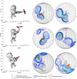
such that the likelihoods of 99% of grasping demonstrations are higher than the threshold. The number of GaussiansKis deter-mined using the Bayesian information criterion (BIC) [36]. Two sets of grasping demonstrations and their graspable probability contour are shown in Figs. 3, 4, 18, and 19.
The likelihood is a measure of the density of feasible grasps in the immediate vicinity. It represents a measure of fitness of a region for grasping. High density (likelihood) in a region results from the fact that this region was more frequently explored by humans; hence, it has a high probability of being a successful grasping location, whereas less- dense regions (likelihood less than a threshold) are bad regions to grasp, as they are rarely seen in the demonstrations. The graspability in these regions is known with much less certainty.
As the graspable-space model of the object is expressed in the object reference frame and the object moves, we provide a simple way of changing the reference frame of the model to the robot’s reference frame by using the following transformation:
rob ot and orientation matrix of the object reference frame (measure-ment frame) with respect to the robot’s base reference frame; Ω (t) = diag (R(t), R(t), R(t))is a9×9 matrix whose diag-onal entries areR(t);zeros(6,1)represents6×1zero vector. For convenience, we will skip the superscriptrobot. Note that in all our experiments, the robot is fixed at the hip, i.e., the robot’s base reference frame does not move.
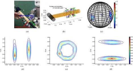
Fig. 3. Modeling the graspable space of a hammer for the iCub hand using a GMM with ten Gaussians. The likelihood contour for end-effector position (d)–(f) andx- andy-directional vectors of orientation (c) with fixed position [0.0; 0.0;−0.035]. (a) Teaching. (b) Grasping configurations for a hammer. (c)ηp o s=(0.0,
0.0, 0.035). (d)ηp o s(3)=0.0. (e)ηp o s(2)=0.0. (f)ηp o s(1)=0.0.
Fig. 4. Modeling the graspable space of a bottle for the Allegro hand using a GMM with 15 Gaussians. The likelihood contour for end-effector position (d)–(f) andx- andy-directional vectors of orientation (d) with fixed position [0.0; 0.0;−0.12]. (a) Allegro hand. (b) Teaching. (c) Grasping samples. (d)ηp o s=(0.0, 0.0,
0.12). (e)ηp o s(3)=0.0. (f)ηp o s(2)=0.0. (g)ηp o s(1)=0.0.
possible motion of the robot’s movement by testing systemati-cally all displacements of its joints. In the case of the iCub, we sample uniformly (ten slices for each joint) its displacement of 7-DOF arm and 3-DOF waist within its respective joint limits.
This yielded a total of 1010 feasible postures in end-effector
postures.
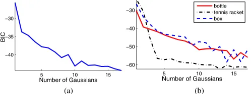
Fig. 5. BIC curves to model the graspable-space models. We determine the number of Gaussians as10for the graspable-space model of a hummer (a) and 15, 13, 14, for the graspable-space model of a bottel, a tennis racket, and a cardboard box, respectively (b). (a) A hammer for iCub hand. (b) For Allegro hand.
distribution of these positions and orientations using GMMs Mreach,{πl, µl,Σl}l= 1:L. Similarly to what was performed for thegraspable-space model, we compute the likelihood of any given pose being reachable.
The optimal numbers of Gaussians for the reachable-space model of the iCub and LWR 4+are determined using BIC [36]. Their BIC curves are shown in Fig. 8. Based on this analysis, the number of Gaussians we determined is23for the reachable-space model of the iCub, and22for the LWR 4+. To verify the accuracy of the reachable-space models, we randomly sample 1 million joint configurations within the joint limits for each robot and evaluate them. Only0.12% (for iCub) and0.13% (for LWR 4+) of samples fell outside the estimated reachable space. In this specific catching experiment with LWR, we discard the reachable samples that are in a condition ofz <0.1m. This en-sures that the robot avoids collision with the table whose surface is the planez= 0. To build a self-collision-free reachable-space model, we conservatively limit the joint ranges. Furthermore, we also discard the reachable samples in which the palm direction is facing toward the ground. Using this way, we discard the undesirable postures without using any heuristics at runtime.
By embedding the set of reachable postures in a probabil-ity densprobabil-ity function, we directly check if a target end-effector posture is reachable, which saves computational time during execution.
3) Predicting Catching Configuration: The graspable-space and reachable-space models explained previously are statisti-cally independent. Hence, we can calculate their joint probabil-ity distribution by simply multiplying the distributions. The joint modelM(t)joint,{π(t)j, µ(t)j,Σ(t)j}j= 1:J, hasJ=K×L number of Gaussians. Each of theJGaussians are expressed as
Σ(t)j =Σ(t)k−1+ Σl−1
In order to find the optimal catching configuration η(t) at a predicted object pose (at a time slice of the pre-dicted trajectory), we use the joint model M(t)joint of
graspable-space and reachable-space models. We compute arg maxη(t)P(η(t)|M(t)joint), through gradient ascent on the
joint model. The Jacobian of this objective function is given by
∂Pη(t)|M(t)joint
We initialize the gradient ascent with the centerµ(t)j of the Gaussian that is closest to the current hand pose (Euclidean distance in 6-D), and we solve this optimization problem. The output of the optimization is a hand pose that has the highest likelihood at the time slice. We compute this for each time slice until the predicted end of flight. The optimal catching configuration and catching time is the configuration and time slice with the highest likelihood. Each time we receive a new measurement of the object’s current pose, we again predict the trajectory and repeat the procedure described previously.
The lengths of the resultant two directional vectors inη(t)ori are not exactly 1. At each step of the gradient ascent method, we normalize the vectors and orthogonalize them so that the resulting rotation matrix is orthonormal. Theoretically, this is a modeling inaccuracy, but because of the reprojection step onto the set of valid rotation matrices, we get a suboptimal but feasible solution.
To reduce the risk that the hand enters in collision with the object, we make sure that the direction of the palm in the catch-ing configuration is opposite from the direction of the object velocity.2This is achieved by requiring the dot product between the direction of the robot’s palm and the negative velocity of the object to be greater than a threshold as the below constraint:
dotη˙(t)p os, η(t)palm< d (12) whereη(t)palmis a palm direction vector [for LWR with Allegro Hand, the palm direction is −η(t)ori,x, see Fig. 4(a)].d is a
direction difference threshold constant. In our experiment, d
was set as0.5, which allows for60.0◦direction difference. This
heuristic constraint greatly decreases the chance of a collision between the robot hand (on the back or side) and the object.
The predicted end-effector pose is mapped into the attractor of the DS-based controller that drives the hand toward the target, and the predicted catching time is set as the desired reaching time in the timing controller [23], as we will explain in the next section.
2Because of the rapid nature of this task, it is not possible to detect and
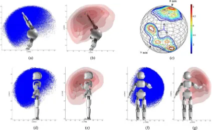
Fig. 6. Modeling of the reachable space for the right arm of the iCub. (a), (d), and (f) Reachable 3-D Cartesian points that are demonstrated from the uniform distribution in joint space. (b), (e), and (g) Probability contour of the reachable-space model that is trained through the Gaussian Mixture Model with 23 Gaussians. (c) Orientation contour when the iCub’s end-effector position [see Fig. 3(a)] is [−0.2, 0.2, 0.45]. (a) Samplesx–y. (b) Modelx–y. (c) Orientation. (d) Samplesx–z. (e) Modelx–z. (f) Samplesy–z. (g) Modely–z.
Fig. 7. Modeling of the reachable space for the LWR 4+. (a), (e), and (g) Reachable 3-D Cartesian points that are demonstrated from the uniform distribution in joint space. (b), (f), and (h) Probability contour of the reachable-space model that is trained through the Gaussian mixture model with 22 Gaussians. (c) and (d) Orientation contour when LWR 4+’s end-effector position [Allegro hand; see Fig. 4(a)] is[−0.13,−0.26,0.79]. (a) Samplesx–y. (b) Modelx–y. (c) Orientation (X-axis). (d) Orientation (Y-axis). (e) Samplesx–z. (f) Modelx–z. (g) Samplesy–z. (h) Modely–z.
C. Hand–Arm Coordinated Motion
We model the trajectories for the end-effector positionξh ∈
R3and orientationξo ∈R3 by using a DS-based model that is learned using thestable estimator of dynamical system(SEDS) technique [20]. The orientation is parameterized using the scaled axis-angle representation asξo ∈R3≡ {ξo1;ξ2o;ξo3}, where the
directionξo represents the axis of rotation, andξorepresents the angle of rotation.
implementation, we achieve the coupling by using the metric ofdistance-to-target. Such a spatial coupling between hand and fingers ensures timely closure of the fingers while following the learned dynamics as closely as possible, even in the presence of arbitrary perturbations.
Here, we briefly summarize the CDS model and the task execution algorithm. For more details, see [38].
1) Model Learning: Letξh ∈R3denote the Cartesian posi-tion of the hand andξf ∈Rdf the joint angles of the fingers.df denotes the total number of DOFs of the fingers. The hand and the fingers follow a separate autonomous DS with associated attractors. For convenience, we place the attractors at the origin of the frames of reference of both the hand motion and the finger motion and, hence, we haveξ∗h = 0andξ∗f = 0. In other words, the hand motion is expressed in a reference frame attached to the object to be grasped, and the zero of the joint angles of the fingers is placed at the joint configuration adopted by the fingers when the object is in the grasp.
The following three joint distributions, learned as separate GMMs, combine to form the CDS model:
1) P(ξh,ξ˙h|θh): encoding the dynamics of the hand trans-port, called themastersubsystem;
2) P(Ψ(ξh),ξf|θinf): encoding the joint probability
distri-bution of the inferred state of the fingers and the current hand position, called theinferencesubsystem;
3) P(ξf,ξ˙f|θf): encoding the dynamics of the finger mo-tion, called theslavesubsystem
Here,Ψ :R3 →Rdenotes thecoupling functionsatisfying
lim
ξh→0
Ψ(ξh) = 0. (13)
θh, θf, and θinf denote the parameter vectors of the GMMs
encoding the master, slave, and the inference models, respec-tively. The distributions in 1) and 3) above are learned by using the SEDS technique [20] that ensures that the learned DS has a single, globally and asymptotically stable attractor. This, in turn, ensures that the overall coupled system will terminate at the desired targets for both the hand pose and the joint angles of the fingers. The probability distribution in 2) does not represent a dynamic3; hence, it is learned using a variant of SEDS where we maximize the likelihood of the model under the constraint
lim
x→0E[ξf|x] =0. (14)
Note that the masterDS runs independently and the slave adapts accordingly to maintain the desired coupling. This im-plies that the dynamics of the reaching motion for the end-effector can be altered without having undesirable effects on the coupling behavior. As explained next, in order to intercept the flying object at the desired instant, we use the timed DS con-troller of [23] for the reaching motion. No change in the other member models of CDS is needed to be compatible with the new reaching dynamics.
2) Trajectory Generation Using Coupled Dynamical Sys-tems: While executing a catching motion, the model essentially
3Here, the dimension of input and output variables is not equal. SEDS can
only be applied to learn the dynamics, where the inputs are positions and outputs are velocities and, thus, have the same dimensionality.
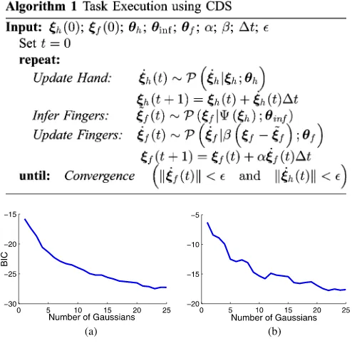
Fig. 8. BIC curves to find the optimal number of a reachable-space model. We determine the number of Gaussians as 23 for the graspable-space model of (a) iCub and 22 for the reachable-space model of (b) LWR 4+. (a) iCub. (b) KUKA LWR 4+.
works in three phases:Update hand pose→Infer finger joints →Increment finger joints. The end-effector pose is generated independently at every time step by using themasterDS. This dynamics is, however, continuously corrected in magnitude with a scalar boost factor so that the robot reaches the catching con-figuration at the desired instant. The change in the boost factor is then set proportional to the difference between the desired reaching time and the reaching time of the currentmasterDS, which is achieved by integrating the DS forward in time (see [23] for detailed description). Subsequently, the current end-effector position is used to modulate the dynamics of the finger motion through the coupling mechanism explained previously. Such a scheme is desired because it ensures that any perturbation is reflected appropriately in both subsystems.
The process starts by generating a velocity command for the hand transport subsystem and increments its state by one time step.Ψ(ξh)transforms the current hand state that is fed to the inference model that calculates the desired state of the joint an-gles of the fingers by conditioning the learned joint distribution. The velocity to drive the finger joints from their current state to the inferred (desired) state is generated byGaussian mixture regressionconditioned on the error between the two. The fingers reach a new state, and the cycle is repeated until convergence. Algorithm 1 explains the complete process in pseudocode, and Fig. 9 shows the closure of the fingers when the robot catches flying objects at different speed.
III. EMPIRICALVALIDATION
Fig. 9. Snapshots of the finger motions when the robot catches objects coming with different speeds. Note that the starting times for finger motion varies with the incoming object speed, i.e., approximately 33 ms (top) versus 50 ms (bottom).
experiments, the state of the fingers was represented byξf ∈R. We use a 1-D finger motion model as this was sufficient for modeling the power grasps used in this study.
A. Implementation in iCub Simulator
Because of hardware limitations in speed and accuracy on the real iCub humanoid robot, we use the iCub simulator [39]. We simulate two objects: a hammer and a tennis racket. In the simulator, each object is thrown 20 times; we randomly change the initial position with the following range,[−2.5±0.5 0.15±0.3 0.8±0.3](m). We also vary the translational veloc-ity between[5.0±2.0 0.0±0.3 3±0.5](m/s), and the angu-lar velocity between[0.0±10 0.0±10 0.0±10](rad/s).
We record the trajectory at 100 Hz. The obtained trajecto-ries are used to train the dynamic model using the SVR tech-nique with the RBF kernel (see Section II-A). We predict the feasible catching configuration and the catching time by us-ing the trained dynamics of the hammer, the graspable-space model (see Section II-B1), and the reachable-space model (see Section II-B2) of the iCub. Various catching configurations of the iCub robot and their orientation contours at the catching position are shown in Fig. 10. The real-time simulation results for the in-flight catching of a hammer and racket are shown in Fig. 11. As real-world uncertainties (such as air drag or measure-ment noise) are not presented in the simulator, the predictions converge very quickly to the true value and are very accurate. To determine the success rate, we perform 50 throws with random initial position, velocity, and angular velocity in the same range with the training throws. The success rate for catching the two objects in simulation is 100%. Note that we excluded the failed throws (three out of the 50 throws) that are not passed into the reachable space of the iCub.
B. Catching Experiment With Real Robot
To validate our method on a real platform, we choose the LWR 4+mounted with the Allegro Hand.4
4Real iCub robot is not fast enough to allow for objects to be caught at the
targeted speed. In the simulator, we boosted the gains to ensure rapid motion.
Fig. 10. iCub could generate different catching configurations. Final catching configuration (left),x-directional contour (middle), andy-directional contour (right) at the catching point.
In the experiments presented here, we use four objects: an empty bottle, a partially filled bottle, a tennis racket, and a cardboard box. In the experiment with a partially filled bottle, we pour 100 g of water inside the empty bottle that weights 33g. To capture both the position and orientation of the object in-flight, we attached three markers to each of the objects. These were captured using theOptitrackmotion capture system from natural point. The position and orientations were captured at 240 Hz.
To train the dynamic models of the moving objects, each ob-ject is thrown 20 times with a varying initial translational and rotational velocity. The trajectories of the measurement frame virtually attached on the object were recorded. Each recorded trajectory is filtered through a Butterworth filter at25Hz. We calculate the velocity and acceleration by using cubic spline in-terpolation. The minimum and maximum values of initial posi-tion, velocity, and angular velocity of the trajectories are shown in Table I in the Appendix. We use SVR-RBF, which are the technique presented in Section II (see [22] for details), to train the dynamics of the objects.
The models of the dynamics of each object are trained sep-arately offline; the trained models are stored in text files so as to use the models in a real-time application. Once a dynamics model is trained, we can predict the position and orientation tra-jectories by measuring the states for a few capturing cycles. The position and orientation accuracy for predictions encompassing 0.5 to 0.0 s is shown in Fig. 12.
Fig. 11. iCub simulation result. The full video is available at http://lasa.epfl.ch/videos/downloads/robotcatchingsim.mp4.
Fig. 12. Prediction error across the four objects in real flight. For each of the objects, ten trajectories are tested. By integrating the estimated acceleration and angular acceleration for the dynamic model, the model predicts future positions and orientations. We varied the amount of data used for prediction from 0.5 to 0.0 s of trajectory time, counting backward from the catching configuration. (a) A bottle. (b) A partially filled bottle. (c) A tennis racket. (d) A cardboard box.
comparison, we place the object coordinate system on the ap-proximated COM. We set as mass for the rigid-body model the weight of the partially filled bottle. We approximate the moment of inertia of the bottle with that of a cylinder. Air drag is ignored. Fig. 13 shows the trajectory of the partially filled bottle. Us-ing the superimposed real trajectory, we show the prediction of the rigid-body model and of nonlinear estimate of the dynam-ics using SVR-RBF. The SVR-RBF predicts the trajectory very accurately. The predictions of the rigid-body dynamics model, in contrast, is very poor, particularly so for the orientation. The discontinuities in the orientation of Fig. 13 come from the
sin-gularity of using Euler angles to represent the orientation (note that the real orientation trajectory of the both models are con-tinuous).
To learn the graspable-space model, we show demonstrations of possible catching hand configurations to the robot. During the demonstrations (around 15 s, 15 (s)×240 (Hz)=3600 catching configuration samples), the positions and orientations of the robot hand and the object are captured using the motion capture system, as shown in Fig. 4(b). Among the recorded catching configurations, 300 samples are randomly selected. The selected samples are trained using GMM. The trained model for grasping a bottle using the Allegro hand is shown in Fig. 4. We also model the reachable space of LWR 4+by using the method introduced in Section II-B2. Using these three models (object dynamics, graspable-space model of the object, and the reachable-space model of the robot), we predict the best catching configuration and the catching time.
Fig. 13. Trajectory of a partially filled bottle and its prediction by using trained SVR-RBF dynamics model and rigid-body dynamics model. (a) Position. (b) Orientation.
Fig. 14. (a) Kinesthetic demonstrations of catching an object. (c) We track the hand and object using the marker-based OptiTrack system. The finger joint angles are recorded synchronously for learning the hand–finger coupling. (d) Human catching the object while the hand position, object position, and finger joint angles are recorded simultaneously.
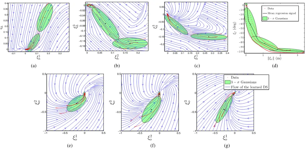
Fig. 15. (a)–(d) Member models of the CDS used to control the Barrett Hand and KUKA LWR arm in coordination to execute the catching motions. (e)–(g) Orientation dynamics estimated using the SEDS technique.
solely using the latter procedure [see Fig. 14(d)], as this would require a remapping of the human data to the nonanthropomor-phic LWR arm. Fig. 15 shows the learned member models of the CDS formulation, i.e., the end-effector position represented byξh ∈R3 ≡ {ξh1;ξh2;ξh3}, the state of the fingers represented byξf ∈R, and the DS encoding the orientation trajectories in the scaled axis-angle representationξo ∈R3 ≡ {ξo1;ξo2;ξo3}.
Fig. 16. Example of trajectory generated by the robot in response to the predicted and real trajectory of the object when catching an empty bottle. The end-effector of the robot continuously adapts to the target and reaches the target on time. In practice, we stop predicting the best catching posture when the predicted time of contact is less than 0.09 s. When the object is very close to the robot, its view from the cameras located in the back of the robot is partially obstructed, yielding a less-accurate estimate of its position. For this reason, we stop predicting the best catching posture when the predicted time at contact is inferior to 0.09 s, which corresponds to a position for the object in the near vicinity of the robot.
updated at every control cycle. The robot continuously adapts the arm and finger motion as the prediction of the final catching configuration improves over time. The output of the position and orientation of the DS is converted into the 7-DOF joint state us-ing the damped least squares IK. We simply choose conservative joint limits for the IK which, in turn, ensure no self-collision. The resultant joint angle is filtered by a critically damped fil-ter to avoid high torques, and the robot is then controlled in joint positions at a rate of 500 Hz. The snapshots of the real robot experiments are shown in Fig. 17. An example of robot end-effector trajectory according to object measurements and predictions of catching posture is shown in Fig. 16.
To compute the rate of success, we throw the empty bottle, the partially filled bottle, the racket, and the cardboard box 20 times each. The prediction of the flying trajectory can start only once the object is visible, i.e., once it enters the region tracked by the motion capture system. This corresponds to an area about 3.5 m from the robot. The average flying time across all trials for the four objects is4.97±0.46(mean±standard deviation) s. Out of 80 trials, we exclude nine trials that never enter the reachable space of the robot. The robot successfully caught the object 52 times out of 71 total trials, yielding a 73.2% success rate.
Failures come in three categories. The first cause of the fail-ures is due to the IK solution for the best catching configuration. If the resulting joint configuration is far away from the initial configuration, the robot cannot reach the target on time, even with its maximum attainable velocity. The CDS and our timing controller generate the Cartesian space end-effector trajectory to bring the end-effector to the target on the desired time, even for the unrespectable prediction change or the dynamically in-feasible target. However, as our CDS in Cartesian space does not take into account the limits of robot in joint space (e.g., joint velocity or torque), it is possible that the robot cannot reach the target at the desired time. This consists of 12 of the 19 failed attempts. Another cause of the failures is when a fin-ger hits the object, which in turn causes the object to bounce away. This happens rarely, and we observe this in four out of 19 failures. The other failures (three out of 19) are caused by vio-lations of the joint torque limits (the robot automatically stops its motion when one of the measured joint torques exceeds the limit).
To compare the success rate of LWR 4+with a human, we performed a catching experiment with a human with the same constraints as the above robotic catching experiment. Ten un-trained subjects (seven males and three females, all of whom are right-handed and between 25 and 32 years old) are asked to stand next to the robot and to catch the object with their right arm, using nothing else than their hand (e.g., all successful catches where the subject catches the object using his chest or upper arm as support are considered to be failed attempts). Step-ping motions are not allowed either. We throw the empty bottle ten times each, totaling 100 throws. The humans successfully caught the object in 38 out of 100 trials, yielding an overall success rate of 10% for the poorest subject to 70% for the best subjects.
IV. DISCUSSION ANDCONCLUSION
Fig. 17. Thrower throws four objects, i.e., a bottle (top), a partially filled bottle (second row), a racket (third row), and a cardboard box (bottom), at around 3.5-m from the robot. The robot catches the bottles in flight. The full video is available at http://lasa.epfl.ch/videos/downloads/kukacatching.mp4.
Fig. 18. Modeling the graspable space of a racket for the Allegro hand using a GMM with 13 Gaussians. The likelihood contour for the end-effector position (e)–(g) andx- andy-directional vectors of orientation (d) with fixed position [0.0; 0.0; 0.035]. (a) A racket, (b) a teaching demonstration, (c) demonstration samples, (d)ηp o s=(0.0, 0.0, 0.035), (e)ηp o s(3)=0.0, (f)ηp o s(2)=0.0, and (g)ηp o s(1)=0.0.
To validate and show the general nature of our method, we perform two different experiments on both the iCub robot (in simulation) and the LWR 4+mounted with an Allegro hand (in real world), very different in terms of the configuration space. We use four objects with very complex dynamics (e.g., a par-tially filled bottle), which leads to a variety of catching config-urations that are difficult to predict and calculate. The average success rate for catching an object in iCub simulation is around
100%, and for the real experiment of LWR 4+, it is approxi-mately 73%. The real robot experiment results are considerably higher than the catching success rate for humans (38%).
Fig. 19. Modeling the graspable space of a bottle for the Allegro hand using a GMM with 14 Gaussians. The likelihood contour for end-effector position (e)–(g); andx- andy-directional vector of orientation (d) with fixed position [−0.125; 0.0; 0.0]. (a) A box, (b) a teaching demonstration, (c) demonstration samples, (d)ηp o s=(0.0, 0.0, 0.12), (e)ηp o s(3)=0.0, (f)ηp o s(2)=0.0, and (g)ηp o s(1)=0.0.
differently compared with the demonstrations, the predicted tra-jectory might be inaccurate. This effect is more pronounced for objects with high nonlinearity in the motion, e.g., a partially filled bottle.
Prediction errors such as the above can possibly lead to an incorrect prediction of the catching configuration. This, in turn, can lead to a catching failure because the robot will start moving in the wrong direction until a better prediction is available. How-ever, as new measurements of the object posture are collected and the future trajectory is reestimated, the catching configura-tion predicconfigura-tion error is reduced gradually.
We use human demonstrations to model the graspable space around an object. Teaching a robot where to grasp via hu-man demonstrations is simple and intuitive. It does not require any prior knowledge about the exact shape, material, and weight of the objects to be grasped. However, only the demon-strated parts of an object can be modeled as possible catching points.
We use probabilistic techniques to model the reachable and graspable spaces. As introduced in Section I, several ways ex-ist to model the reachable space, e.g., numerical modeling, databases, or density-based modeling. To our knowledge, how-ever, there are no generalized methods for building a continuous model of the 6-D reachable and graspable space and that can be queried in real time. Using a probabilistic encoding to model the graspable and reachable spaces has several benefits. It provides us with a notion of the likelihood from which we can determine the most likely catching point. It can easily be rotated and trans-lated so as to perform the computation online in the moving object’s frame of reference.
To ensure timely and rapid computation time, whenever pos-sible, we find closed-form expressions for each computational step. We show that the overall computation is extremely rapid, thus enabling us to compute the best catching configuration in around 0.2 ms (on 2.7-GHz quad-core PC) and to catch objects when the overall flying time does not exceed 0.7 s.
The choice of modeling reachable and graspable space with positive examples is inspired by the one-class classification scheme where there are only data from the positive class, and there is an attempt to fit a boundary around it as tightly as possi-ble. Although this procedure can generate some false negatives (feasible regions decided as infeasible by the model), it is highly unlikely to generate false positives (infeasible regions decided as feasible). The frequency of such errors can be further de-creased by making the threshold (currently 99%) even lower. We find that, in practice, setting the threshold to 99% does not yield to sample infeasible regions.
As we model the reachable space through a joint-probability distribution, we can compute conditional probability on all vari-ables. For example, when a robot needs to grasp a static object at a specific position, the feasible orientations can be computed simply by conditioning the orientation on the position. We can also compute the likelihood of each of the marginal distribu-tions to determine separately the likelihood of the position and orientation. We can, for instance, determine the reachability of a given 3-D position while ignoring orientation. This can be useful when only the position is relevant, such as when catching a ball.
TABLE I
INITIALSVALUES OF THETHROWINGDEMONSTRATIONS
that need improvement. For starters, we consider only catching motions that stop at the target. This results in the object bouncing off after hitting the robot’s hand. This is undesirable, especially as the object can produce a strong impact force on the hand, which can lead to damage. Addressing the shortcomings with compliant catching will be our next challenge.
As mentioned in the main text of the paper, we do not explic-itly compute collisions, before catching, between the object and the hand and arm. Although we prevent this from happening through simple heuristics (opposite orientation of the palm to the object velocity vector), this is not sufficient and leads to a few cases of failures in the experiments. We conservatively limit the joint ranges to avoid self-collision when modeling the reach-able space and in solving IK. This reduces the usreach-able reachreach-able space of a robot. Recently, a real-time optimization method was applied to a robotic catching task to avoid self-collisions and environment-collisions, to avoid joint limits (position and ve-locity), and to find smooth joint angle trajectories. However, it requires a large amount of computational power (Baumlet al.[4] use external 32-core high-performance computer in a ball catch-ing experiment). Indeed, computcatch-ing obstacle avoidance in real time for catching complex objects is a very challenging task, and we do not yet have a solution to this problem. These is-sues are open isis-sues in robotics, and we consider them as future work.
The graspable model is used solely to learn power grasps. Precision grasps might be interesting for catching very small objects. It would be possible to extend the GMM approach to embed a representation of the grasping points on each finger, as a triplet, by expanding the space of control.
Finally, and perhaps most importantly, we model solely the dynamics of the task and do not model the robot’s dynamics. As a result, some of the trajectories generated by our CDS model lead to generate velocities that the robot could not follow. This is the third cause of failure to catch the objects in the real experiment. A potential direction to address this issue would be to generate dynamically feasible trajectories from optimal control (in place of using human demonstrations) to populate the CDS model with examples of motion that satisfy the dynamics of the robot. These problems remain for potential resolution in future work.
APPENDIX
See Table I, which shows the initial values of the throwing demonstrations.
REFERENCES
[1] J. Aleotti and S. Caselli, “Robust trajectory learning and approximation for robot programming by demonstration,”Robot. Auton. Syst., vol. 54, no. 5, pp. 409–413, 2006.
[2] J. Bae, S. Park, J. Park, M. Baeg, D. Kim, and S. Oh, “Development of a low cost anthropomorphic robot hand with high capability,” inProc. IEEE/RSJ Int. Conf. Intell. Robot. Syst., 2012, pp. 4776–4782.
[3] A. L. Barker, D. E. Brown, and W. N. Martin, “Bayesian estimation and the Kalman filter,”Comput. Math. Appl., vol. 30, no. 10, pp. 55–77, 1995. [4] B. Bauml, T. Wimbock, and G. Hirzinger, “Kinematically optimal catching a flying ball with a hand-arm-system,” inProc. IEEE/RSJ Int. Conf. Intell. Robot. Syst., 2010, pp. 2592–2599.
[5] K. S. Bhat, S. M. Seitz, J. Popovic, and P. K. Khosla, “Computing the physical parameters of rigid-body motion from video,” inProc. 7th Eur. Conf. Comput. Vision, 2002, pp. 551–565.
[6] M. Buehler, D. E. Koditschek, and P. J. Kindlmann, “Planning and control of robotic juggling and catching tasks,”Int. J. Robot. Res., vol. 13, no. 12, pp. 101–118, Apr. 1994.
[7] S. Calinon, F. Guenter, and A. Billard, “On learning, representing and generalizing a task in a humanoid robot,”IEEE Trans. Syst., Man, Cybern. B, Cybern., vol. 37, no. 2, pp. 286–298, Apr. 2007.
[8] C.-C. Chang and C.-J. Lin, “LIBSVM: A library for support vector ma-chines,”ACM Trans. Intell. Syst. Technol., vol. 2, pp. 27:1–27:27, 2011. [9] G. Chirikjian and I. Ebert-Uphoff, “Numerical convolution on the
Eu-clidean group with applications to workspace generation,”IEEE Trans. Robot. Autom., vol. 14, no. 1, pp. 123–136, Feb. 1998.
[10] A. P. Dempster, N. M. Laird, and D. B. Rubin, “Maximum likelihood from incomplete data via the EM algorithm,”J. Roy. Statist. Soc. Series B (Methodol.), vol. 39, no. 1, pp. 1–38, 1977.
[11] R. Detry, D. Kraft, O. Kroemer, L. Bodenhagen, J. Peters, N. Kruger, and J. Piater, “Learning grasp affordance densities,”J. Behav. Robot., vol. 2, no. 1, pp. 1–17, 2011.
[12] R. Diankov, N. Ratliff, D. Ferguson, S. Srinivasa, and J. Kuffner, “Bispace planning: Concurrent multi-space exploration,”Robot.: Sci. Syst., pp. 159-166, 2008.
[13] U. Frese, B. Bauml, S. Haidacher, G. Schreiber, I. Schaefer, M. Hahnle, and G. Hirzinger, “Off-the-shelf vision for a robotic ball catcher,” inProc. IEEE/RSJ Int. Conf. Intell. Robot. Syst., 2001, vol. 3, pp. 1623–1629. [14] E. Gribovskaya, S.-M. Khansari-Zadeh, and A. Billard, “Learning
non-linear multivariate dynamics of motion in robotic manipulators,”Int. J. Robot. Res., 2010.
[15] Y. Guan and K. Yokoi, “Reachable boundary of a humanoid robot with two feet fixed on the ground,” inProc. IEEE Int. Conf. Robot. Autom., 2006, pp. 1518–1523.
[16] Y. Guan and K. Yokoi, “Reachable space generation of a humanoid robot using the Monte Carlo method,” inProc. IEEE/RSJ Int. Conf. Intell. Robot. Syst., 2006, pp. 1984–1989.
[17] L. Guilamo, J. Kuffner, K. Nishiwaki, and S. Kagami, “Efficient prior-itized inverse kinematic solutions for redundant manipulators,” inProc. IEEE/RSJ Int. Conf. Intell. Robot. Syst., 2005, pp. 3921–3926.
[18] W. Hong and J.-J. E. Slotine, “Experiments in hand-eye coordination using active vision,” inProc. 4th Int. Symp. Exp. Robot. IV., London, UK: Springer-Verlag, 1997, pp. 130–139.
[19] J. Hwang, R. C. Arkin, and D. Kwon, “Mobile robots at your fingertip: Bezier curve on-line trajectory generation for supervisory control,” in
Proc. IEEE/RSJ Int. Conf. Intell. Robot. Syst., 2003, vol. 2, pp. 1444– 1449.
[21] S.-M. Khansari-Zadeh and A. Billard, “A dynamical system approach to realtime obstacle avoidance,”Auton. Robots, vol. 32, pp. 433–454, 2012. [22] S. Kim and A. Billard, “Estimating the non-linear dynamics of free-flying
objects,”Robot. Auton. Syst., vol. 60, no. 9, pp. 1108–1122, 2012. [23] S. Kim, E. Gribovskaya, and A. Billard, “Learning motion dynamics to
catch a moving object,” inProc. 10th IEEE-RAS Int. Conf. Humanoid Robots, 2010.
[24] J. Kober, K. Mulling, O. Kromer, C. H. Lampert, B. Scholkopf, and J. Peters, “Movement templates for learning of hitting and batting,” in
Proc. IEEE Int. Conf. Robot. Autom., 2010, pp. 853–858.
[25] J. Kober, M. Glisson, and M. Mistry, “Playing catch and juggling with a humanoid robot,” inProc. IEEE-RAS Int. Conf. Humanoid Robots, Osaka, Japan, 2012, pp. 875–881.
[26] S.-J. Kwon and Y. Youm, “General algorithm for automatic generation of the workspace for n-link redundant manipulators,” inProc. Int. Conf. Adv. Robot., 1991, vol. 1, pp. 1722–1725.
[27] K. J. Kyriakopoulos and G. N. Saridis, “Minimum jerk path generation,” inProc. IEEE Int. Conf. Robot. Autom., 1988, pp. 364–369.
[28] R. Lampariello, D. Nguyen-Tuong, C. Castellini, G. Hirzinger, and J. Peters, “Trajectory planning for optimal robot catching in real-time,” in
Proc. Int. Conf. Robot. Autom., 2011, pp. 3719–3726.
[29] J.-P. Merlet, C. M. Gosselin, and N. Mouly, “Workspaces of planar parallel manipulators,”Mech. Mach. Theory, vol. 33, no. 1–2, pp. 7–20, 1998. [30] A. Namiki and M. Ishikawa, “Robotic catching using a direct mapping
from visual information to motor command,” inProc. IEEE Int. Conf. Robot. Autom., 2003, vol. 2, pp. 2400–2405.
[31] G. Park, K. Kim, C. Kim, M. Jeong, B. You, and S. Ra, “Human-like catch-ing motion of humanoid uscatch-ing evolutionary algorithm(ea)-based imitation learning,” inProc. IEEE Int. Sympo. Robot Human Interact. Commun., 2009, pp. 809–815.
[32] M. Riley and C. G. Atkeson, “Robot catching: Towards engaging human-humanoid interaction,”Auton. Robots, vol. 12, no. 1, pp. 119–128, 2002. [33] A. Rizzi and D. Koditschek, “Further progress in robot juggling: Solv-able mirror laws,” inProc. IEEE Int. Conf. Robot. Autom., 1994, vol. 4, pp. 2935–2940.
[34] S. Schaal and D. Sternad, “Programmable pattern generators,” inProc. Int. Conf. Comput. Intell. Neurosci., 1998, pp. 48–51.
[35] S. Schaal, D. Sternad, and C. G. Atkeson, “One-handed juggling: A dy-namical approach to a rhythmic movement task,”J. Motor Behav., vol. 28, pp. 165–183, 1996.
[36] G. Schwarz, “Estimating the dimension of a model,”Ann. Statist., vol. 6, no. 2, pp. 461–464, 1978.
[37] T. Senoo, A. Namiki, and M. Ishikawa, “Ball control in high-speed batting motion using hybrid trajectory generator,” inProc. IEEE Int. Conf. Robot. Autom., 2006, pp. 1762–1767.
[38] A. Shukla and A. Billard, “Coupled dynamical system based armhand grasping model for learning fast adaptation strategies,”Robot. Auton. Syst., vol. 60, no. 3, pp. 424–440, 2012.
[39] V. Tikhanoff, A. Cangelosi, P. Fitzpatrick, G. Metta, L. Natale, and F. Nori, “An open-source simulator for cognitive robotics research: The prototype of the iCub humanoid robot simulator,” inProc. 8th Workshop Perfor-mance Metrics Intell. Syst., 2008, pp. 57–61.
[40] Y. Wang and G. Chirikjian, “A diffusion-based algorithm for workspace generation of highly articulated manipulators,” inProc. IEEE Int. Conf. Robot. Autom., 2002, pp. 1525–1530.
[41] F. Zacharias, C. Borst, and G. Hirzinger, “Capturing robot workspace structure: Representing robot capabilities,,” inProc. IEEE/RSJ Int. Conf. Intell. Robot. Syst., 2007, pp. 3229–3236.
[42] F. Zacharias, C. Borst, and G. Hirzinger, “Object-specific grasp maps for use in planning manipulation actions,” inAdvances in Robotics Research. Berlin, Germany: Springer, 2009, pp. 203–213.
[43] H. Zhang, “Efficient evaluation of the feasibility of robot displacement trajectories,”IEEE Trans. Syst., Man, Cybern., vol. 23, no. 1, pp. 324– 330, Jan./Feb. 1993.
[44] M. Zhang and M. Buehler, “Sensor-based online trajectory generation for smoothly grasping moving objects,” inProc. IEEE Int. Symp. Intell. Control, 1994, pp. 16–18.
Seungsu Kimreceived the B.Sc. and M.Sc. degrees in mechanical engineering from Hanyang University, Seoul, Korea, in 2005 and 2007, respectively, and the Ph.D. degree in robotics from the Swiss Federal Insti-tute of Technology in Lausanne (EPFL), Lausanne, Switzerland, in 2014.
He is currently a Postdoctoral Fellow with the Learning Algorithms and Systems Laboratory, EPFL. He was a Researcher with the Center for Cognitive Robotics Research, Korea Institute of Science and Technology, Daejeon, Korea, from 2005 to 2009. His research interests include machine-learning techniques for robot manipulation.
Ashwini Shuklareceived the Bachelor’s and Mas-ter’s degrees in mechanical engineering from the In-dian Institute of Technology, Kanpur, India, in 2009. He is currently working toward the Ph.D. degree with the Learning Algorithms and Systems Laboratory, Swiss Federal Institute of Technology in Lausanne, Lausanne, Switzerland.
His research interests include programming by demonstration and machine-learning techniques for robot control and planning.
Aude Billardreceived the M.Sc. degree in physics from the Swiss Federal Institute of Technology in Lausanne (EPFL), Lausanne, Switzerland, in 1995, and the M.Sc. degree in knowledge-based systems and the Ph.D. degree in artificial intelligence from the University of Edinburgh, Edinburgh, U.K., in 1996 and 1998, respectively.
She is currently a Professor of micro and mechan-ical Engineering and the Head of the Learning Algo-rithms and Systems Laboratory, School of Engineer-ing, EPFL. Her research interests include machine-learning tools to support robot machine-learning through human guidance. This also extends to research on complementary topics, including machine vision and its use in human–robot interaction and computational neuroscience to develop models of motor learning in humans.