*Corresponding author. Tel.:#1-604-822-8484; fax:#1-604-822-8477. E-mail address:[email protected] (W. Antweiler).
Nested random e!ects estimation in
unbalanced panel data
Werner Antweiler*
Faculty of Commerce, The University of British Columbia, 2053 Main Mall, Vancouver, BC Canada V6T 1Z2
Received 27 October 1997; received in revised form 26 July 2000; accepted 2 October 2000
Abstract
Panel data in many econometric applications exhibit a nested (hierarchical) structure.
For example, data on"rms may be grouped by industry, or data on air pollution may be
grouped by observation station within a city, city within a country, and by country. In these cases, one can control for unobserved group and sub-group e!ects using a nested-error component model. A double-nested unbalanced panel is examined and a corresponding maximum likelihood estimator is derived. A generalization to even higher-order nesting is feasible. A practical example and a Monte-Carlo simulation compare the new estimator against the non-nested ML estimator. The style of presenta-tion is intended to aid applied econometricians in implementing the new ML
estimator. ( 2001 Elsevier Science S.A. All rights reserved.
JEL classixcation: C13; C23
Keywords: Panel data; Nested e!ects; Error component model; Econometrics
1. Introduction and motivation
Data often exhibit a nested (or hierarchical) structure. For example,"rms may be grouped by industry. This is a single-nested structure. Data on air pollution
1For single-nested panels one alternative is the estimation of&mixed e!ects'where a"xed-e!ects approach is used for the top-level group (e.g. countries) and a random-e!ects approach is used for the low-level group (e.g. cities). This method may be appropriate in cases where the top level covers an entire population (such as all industries in an economy or all countries in the world); in other cases, however, this method may be inappropriate.
may be grouped by observation station within a city and city within a country. This is a double-nested structure. Although there can be any number of nestings, most applications will be of the single-or double-nested type. This paper ex-plores the double-nested error component model, but estimators for higher-order nestings can be obtained using the methodology presented here. This paper is aimed at the econometric practitioner. Therefore, care has been taken to use notation that will allow the practitioner to implement the methods described in this paper into suitable econometric software. In what follows, Section 2 provides a brief overview of the literature on nested panels and motivates the analysis by presenting the case of balanced panels. Section 3 addresses the more complex case of unbalanced panels and introduces a suitable maximum likeli-hood (ML) estimator. A concrete example is provided in Section 4 where this new ML estimator for double-nested panels is compared to the non-nested panel ML estimator. Section 5 concludes with a small Monte-Carlo study of the new ML estimator.
While the problem of hierarchical panels appears to be one of great practical importance, not much work has been published on this topic. Early work on balanced panels include Ghosh (1976), who developed an ANOVA-type es-timator for single-nested panels, and Fuller and Battese (1973), who investigated the error structure of double-nested data sets with cross-sectional data but no time dimension. This was later improved upon by Baltagi (1987). Pakes (1983) discusses regression analysis where populations are grouped. Searle (1987, Chapter 3) discusses nested data structures in a variance analysis context. It appears that Baltagi (1993)"rst proposed the term`nested e!ects,aadapting the term `nested-error structurea by Fuller and Battese (1973) to the context of panel data.
New and complementary work to this paper appears in Baltagi et al. (1999a, b) and Davis (1999).
One econometric problem in data sets with a nested structure relates to the possibility that individual e!ects may be associated with each level. For example, in a model with cities and countries there can be city-speci"c e!ects as well as country-speci"c e!ects. Using country-speci"c e!ects alone would ex-clude the possibility of city-speci"c e!ects, and vice versa.1
2See Moulton (1986, 1987, 1990).
well-known Moulton bias in standard errors.2There are two issues. First, the standard errors computed under the assumption that the error term is i.i.d. will be biased (downward if the error terms are positively correlated). Second, the assumption of independence is unlikely to be satis"ed when aggregate (macro) data are merged with micro data. For example, it is common in labour econ-omics to merge micro data on individual workers with macro data on industry, occupation, or geographic location. More concretely, estimation of a wage equation for individual workers could involve characteristics of the individual worker as well as aggregate (e.g., state or country) unemployment rates.
Consider a regression equation
y
ijkt"x@ijktb#uijkt, (1)
fori"1,2,¸; j"1,2,Mi;k"1,2,Nijandt"1,2,¹ijk. For example, the
dependent variabley
ijktcould denote the air pollution measured at stationkin
cityjof countryiin time periodt. This means that there are¸countries, and each country ihasM
i cities in whichNij observation stations are located. At
such a station, air pollution is observed during¹
ijk periods. Thexijkt denotes
a vector ofK explanatory variables, and the disturbance is given by
u
ijkt"ji#kij#lijk#eijkt, (2)
wherej
i&IID(0,p2j),kij&IID(0,p2k),lijk&IID(0,p2l), and eijkt&IID(0,p2e),
are independent of each other and among themselves. When considering the ML estimator, the assumption of normality will be added.
2. Nested balanced panels
The"rst reference of a nested error structure can be found in Ghosh (1976). This study considers a balanced panel with a single-nested (e.g., country and region) structure as well as individual time e!ects. Baltagi (1987), using meth-odology developed by Wansbeek and Kapteyn (1982), provides a more rigorous algebraic derivation of this type of estimator based on the spectral decomposi-tion of the variance}covariance matrixX.
Xiong (1995) elegantly derives a nested-e!ects estimator for single-nested balanced panels (without separate time e!ects). I generalize this estimator to the nested case to provide a reference point for the discussion of the double-nested unbalanced panel in Section 3. To begin with, letI
sbe an identity matrix
of dimensions, and letJ
sbe a square matrix of dimensionswith all elements 1,
and for convenience of algebraic manipulation, introduce P
3For scalarsf
iand an arbitrary scalarr, it holds thatXr"+ifriZi when the matricesZiare pairwise orthogonal to each other and sum to the identity matrix, and eachZ
iis symmetric and idempotent with its rank equal to its trace. See Nerlove (1971b).
Q
s,Is!Ps. Also note thatIrs"Ir ?Is andPrs"Pr ?Ps for any positive
integersr and s. Expressing (2) in matrix form and computing X"E(uu@), it follows that
X"p2
j(IL?JMNT)#p2k(ILM?JNT)#p2l(ILMN?JT)#p2eILMNT. (3)
First transforming the Jmatrices into Pmatrices, then recursively expanding the multi-group I matrices into the sum of P and Q matrices, collapsing contiguousPmatrices, and"nally collecting terms, yields
X"MN¹p2j(I
L?PMNT)#N¹p2k(ILM?PNT)#¹p2l(ILMN?PT)#p2eILMNT
"(MN¹p2
j#N¹p2k#¹pl2#p2e)(IL?PMNT)
#(N¹p2k#¹p2
l#p2e)(IL?QM?PNT)
#(¹p2l#p2
e)(ILM?QN?PT)#p2e(ILMN?QT)
"p2
e(ILMN?QT)#p21(ILM?QN?PT)#p22(IL?QM?PNT)
#p2
3(IL?PMNT), (4)
where in the last linep2e, p21, p22, andp23 were introduced as the characteristic roots of the spectral decomposition ofX. They are de"ned as follows:
p21,¹p2
l#p2e, (5)
p22,N¹p2
k#¹p2l#p2e, (6) p23,MN¹p2j#N¹p2k#¹p2
l#p2e. (7) As the terms with the Kronecker products are all orthogonal to each other and sum to I
LMNT, it follows that3 X~1@2"p~1
e (ILMN?QT)#p1~1(ILM?QN?PT)
#p~1
2 (IL?QM?PNT)#p~13 (IL?PMNT). (8)
Now expand all theQmatrices as the di!erence ofIandP, multiply both sides of the equation bype, and collect terms
peX~1@2"I
LMNT!
A
1!pe
p1
B
(ILMN?PT)!
A
pe p1!pe
p2
B
(ILM?PNT)!A
pe p2!
pe
4For a discussion, see Baltagi (1995, Chapter 9), and in particular, Wansbeek and Kapteyn (1989). 5Computational cost is hardly a consideration anymore.
6For the latter, see Maddala and Mount (1973). Also see Section 5 below.
To perform generalized least squares, the following transformed system ofy(and likewisex) is estimated via OLS:
yH
ijkt"yijkt!
A
1!pe
p1
B
y6ijkv!A
pe p1!
pe
p2
B
y6ijvv!A
pe p2!
pe p3
B
y6ivvv,(10)
wherey6ijkv, y6ijvv, andy6ivvvindicate group averages. The pattern exhibited in Eq. (10) is suggestive of solutions for higher-order nested panels. For feasible generalized least squares, estimates of the variances can be obtained from the three group-wise between estimators and the within estimator for the innermost group.
3. An ML estimator for unbalanced panels
Unbalanced panels cannot be handled easily in the framework developed in the previous section. The Kronecker product can only be used in the case of balanced panels. Thus, unbalanced panels introduce quite a bit of notational inconvenience into the algebra.4At the same time, it will become apparent that unbalanced panels cannot be easily moulded into a feasible generalized least squares (FGLS) transformation for OLS estimation. Provided that introducing the normality assumption on the error structure is unproblematic in the given application, maximum likelihood estimation provides a suitable alternative.5
Two other points make ML estimation appealing: the variances are estimated directly, and ML generally performs well for unbalanced panels.6
In deriving a practical estimator for nested panels, the key challenge is"nding an expression forX~1that is computationally feasible. The expression I derive below turns out to be just that, and by exploiting the recursive nature of the panel's hierarchic structure it suggests an immediate generalization to arbitrary orders of nesting.
I begin by introducing some notation and de"ning certain types of matrices that are used in the derivation of an inverse and determinant ofX. An unbal-anced panel is made up of¸top level groups, each containingM
i second-level
groups. The second-level groups contain the innermostN
ijsubgroups, which in
turn contain¹
ijk observations. The number of observations in the higher-level
groups are thus ¹
observations isH,+Li/1¹
i. The number of top-level groups is¸, the number of
second-level groups isF,+Li/1M
i, and the number of bottom-level groups is
G,+Li/1+Mi
j/1Nij.
For balanced panels it was possible to neatly stack theJmatrices of all&1's using I?J products. For unbalanced panels I rede"ne the J matrices to be blockdiagonal of size H]H, corresponding in structure to the groups or subgroups they represent. They can be constructed explicitly by using`group membershipamatrices consisting of ones and zeros that uniquely assign each of theHobservations to one of theG(orFor¸) groups. LetRlbe such anH]G matrix corresponding to the innermost group level. Then the blockdiagonal H]H matrix Jl can be expressed as the outer product of its membership matrices:J
l"RlR@l. Further note that the inner productR@lRlproduces a diag-onal matrix¹I
lof sizeG]Gthat contains the number of observations for each group. Similarly,¹I
k"R@kRk. In what follows the tilde accent will always denote such an`interioramatrix corresponding to the`exterioraH]Hmatrix of the same name. De"ne ¹
l as an H]H matrix of observations with elements ¹
l,ijkt"¹ijk, and then it is apparent thatRl¹Il"¹lRl. De"ne¹kanalogously as theH]Hmatrix corresponding to theF]Fmatrix¹I
k. The properties of the ¹ and J matrices can be exploited advantageously. Note that JlJl"Rl(R@lRl)R@l"Rl¹I
lR@l"¹lJl. Similarly,JkJk"¹kJk.
The mapping from groups to subgroups can also be captured through membership matrices. Let Rlk,R@
kRl¹I~1l be an F]G matrix mapping Fgroups toGsubgroups. De"neRkjcorrespondingly as an¸]Fmatrix. Also note the recursive nature of the mapping process:Rk"Rl(Rlk)@.
Similar to theP matrices that were de"ned for balanced panels, projection matrix P
l,Rl¹I~1l Rl@"¹~1l Jl is idempotent: PlPl"Rl¹I~1l R@lRl¹I~1l R@l" R
l(¹I~1l ¹Il)¹I~1l R@l"Pl. The second property of this projection matrix estab-lishes that such a matrix can be pre- or post-multiplied with aJorPmatrix of
equal nesting without changing it, for example, P
lJl"Rl¹I~1l R@lRlR@l" R
l¹I~1l ¹IlR@l"RlR@l"Jl. Using this second property I establish the third property which allows a projection matrix to be applied to a J or P of
higher-order nesting without changing it: PlJk"PlPkJk" (Rl¹I~1
l R@l)(Rk¹I~1k R@k)Jk"¹~1l (RlR@l)(RkR@k)¹~1k Jk"(¹~1l ¹l)(¹~1k ¹k)Jk"Jk. Now it is apparent thatJlJk"¹
lJk, and analogously, JkJl"Jk¹l. To see this, observe that by constructionJl"¹
lPl, and thatPlJk"Jk by property 3 of the projection matrix.
In the next step I introduce a further type of matrix. It will turn out that the diagonalSmatrices introduced here are made up of eigenvalues of yet another type of matrix (theZmatrices) introduced later. Let
Sl,I#o
l¹l, (11)
S
k,I#okUk, (12) S
7By comparison, the matrices with the tilde accent contain one unique value for each group, while the matrices without a tilde accent replicate the value from each group for all observations in that group.
8See also Baltagi (1995, Chapters 2.4 and 3.4) and Hsiao (1986, Chapter 3.3.3).
where U
k and Uj are diagonal matrices with elements Uk,ijkt"/ij and U
j,ijkt"/i. The elements of theSandUmatrices are de"ned recursively
hijk,1#ol¹
ijk, /ij, Nij + k/1
¹
ijk
hijk, hij,1#ok/ij, /i, Mi + j/1
/ ij
hij,
hi,1#oj/ i
whereol,p2
l/p2e,ok,p2j/p2e, andoj,p2j/p2e are variance ratios.
For the following proofs it is helpful to consider theG]G, F]F, and¸]¸
`interioracounterparts of theSandUmatrices; they are indicated again by a tilde accent on their top.7 Corresponding to (11)}(13) are SIl"I
G#ol¹Il;
SIk"I
F#okUIk; andSIj"IL#ojUIj. The UI matrices can then be derived as
follows:
UIk"RlkSI~1l ¹I
lRl@k"R@kRlSI~1l ¹Il~1R@lRk"R@kS~1l Rk, (14)
UIj"RkjSI~1k UIkRk@j"R@
jRk¹~1k (R@kS~1l Rk)SI~1k ¹~1k R@kRj
"R@jS~1k S~1l Rj. (15) In the above simpli"cations it should be noted thatRlSIl"SlRl, RkSIk"SkRk, andR
jSIj"SjRj. Also remember thatRk¹I~1k R@kis an idempotent matrix and thatP
kRk"Rk.Smatrices andJmatrices commute in one special case: ifScan be represented by an`interioramatrixSthat corresponds to the nesting level of J. This means that the commutativity holds only when for each block in the Jmatrix the corresponding elements in theSmatrix are all the same. Thus it is true that SkJk"JkSk, but note that SlJkOJkSl. Also, SkJl"JlSk. To see this, consider the case whereSkJk"SkRkR@k"RkSIkR@k"RkR@kSk"JkSk. As long as S of size H]H is reducible to SI of size F]F corresponding to R, commutativity is guaranteed.
Having dealt with these preliminaries, the variance}covariance matrix for an unbalanced panel can be written as
X"p2
e[I#olJl#okJk#ojJj]. (16)
The log-likelihood function L corresponding to the error structure given in
(2) is8
L"!1
9Note that the following is a highly specialized version of rule 19.18 in Sydsvter et al. (1999, p. 125).
There are thus two challenges: computing the determinantDXDand the inverse
X~1. The following technique can be used to tackle these two challenges. Introduce
Zl,I#o
lJl, (18)
Z
k,I#Z~1l okJk"I#S~1l okJk, (19) Zj,I#Z~1k Z~1l ojJj"I#S~1k S~1l ojJj, (20) so that instead of writing (16) as a sum it can be written as the product
X"Z
lZkZj, which is veri"ed by substituting (18)}(20) into this expression and expanding. Notice the introduction of theSmatrices in (19)}(20). They are direct counterparts to theZmatrices, but unlike these, theSmatrices are diagonal and made up of eigenvalues of the correspondingZmatrices. Proving the equality parts of (19)}(20) is the primary challenge. It is now apparent that
DXD"(p2
e)HDZlDDZkDDZjD, (21)
X~1"Z~1j Z~1k Z~1l /p2e, (22) and it needs to be shown that9
Z~1l "I!Z~1l olJl"I!S~1l olJl, (23) Z~1k "I!Z~1k Z~1l okJ
k"I!S~1k S~1l okJk, (24) Z~1j "I!Z~1j Z~1k Z~1l ojJj"I!S~1j S~1k S~1l ojJj. (25) It is easily veri"ed that the left and middle expressions in (23)}(25) are identical. By construction Z~1l Z
l"I, Z~1k Zk"I, and Z~1j Zj"I. In the "rst case, rearranging expressions yieldsZ~1l (I#olJ
l)"I, where the part in parenthesis is of courseZl. The other two cases work analogously. The remaining task is to show the equality of the middle and right parts of (23)}(25). I will only show the most di$cult case (25); the two simpler cases are embedded within. Proving (25) is equivalent to demonstrating that
J
j"ZlZkZjSj~1S~1k S~1l Jj, "[I#o
lJl#okJk#ojJj]S~1j S~1k S~1l Jj, "S~1j [S~1k (S~1l (J
j#olJlJj)#okJkS~1l Jj)#ojJjS~1k S~1l Jj], (26) "S~1j [S~1k (S~1l (Jj#o
"S~1j [S~1k (S~1l (I#ol¹
l)#okUk)#ojUj]Jj, "S~1j [S~1k (I#o
kUk)#ojUj]Jj, "S~1j [I#o
jUj]Jj, "Jj.
Arriving at step (26) simply makes use of the commutativity of the S and Jmatrices. The crucial step from (26) to (27) makes use of three equalities. First, it was shown earlier that JlJl"¹
lJl. Second, using the simpli"cation from (14), it is true that JkS~1l Jj"Rk(R@kS~1l Rk)¹I~1
k R@kJj"RkUIk¹I~1k R@kJj"
UkPkJj"UkJj. And third,JjS~1k S~1l Jj"UjJj is trivially true from (15). The above proof is also helpful in the following step. Using the same tech-nique it can be shown thatJjZ~1k Z~1l "JjS~1k S~1l andJkZ~1l "JkS~1l . I use these equalities below in proceeding from steps (28) to (29) when I expand and simplifyp2eX~1:
Z~1j Z~1k Z~1l "Z~1k Z~1l !S~1j S~1k S~1l J
jZ~1k Z~1l ,
"Z~1l !S~1k S~1l okJkZ~1l !S~1j S~1k S~1l JjZ~1k Z~1l , "I!S~1l olJl!S~1k S~1l okJkZ~1l !S~1j S~1k S~1l JjZ~1k Z~1l ,
(28)
"I!S~1l olJl!S~1k S~1l okJkS~1l !S~1j S~1k S~1l JjS~1k S~1l . (29)
In passing I note the di$culty of"nding a simple projection matrixCsatisfying
C@C"X~1 that would produce an observation-by-observation GLS-to-OLS
transformation. The Jk andJj matrices are bordered on both sides by some non-commutableSmatrices. Thus, an observation-by-observation transforma-tion cannot be obtained from (29) except in the non-nested case where ok"o
j"0.
In the next step I derive the determinant ofX. The following lemma applies to the sum of the identity matrix and the product of an arbitrary diagonal matrix Dand a block-diagonalJmatrix stacked withk"1,2,Nblocks of 1's with size ¹
k]¹k.
DI#oDJD"<N
k/1
A
1#oT+k t/1
d
kt
B
. (30)This lemma can be applied immediately to (18). In the case of (19) and (20), it is true thatZ~1l J
k"S~1l JkandZ~1k Z~1l Jj"S~1k S~1l Jj. ThenDXDcan be written as follows:
DXD"(p2e)H<L
i/1
h
i Mi <
j/1
h
ij Nij <
k/1
h
10While an analytic gradient is not strictly necessary for computational purposes (as many software packages provide numeric approximations), they signi"cantly speed up computations. Even with an analytic gradient, however, the Hessian matrixW is typically obtained through numeric approximation methods.Wis used to obtain standard errorss
bfor the estimates of the
Bregressors. The diagonal elements of the inverse of the Hessian, corrected for the degrees of freedom, are approximately following at-distribution withH!G!Bdegrees of freedom. More formally, this can be expressed ass
b"Jabs([W~1H/(H!G!B)]bb)&t(H!G!B).
In the case of a balanced panel,DXD simpli"es to
DXD"(p2e)H(1#ol¹)LM(N~1)(1#ol¹#o
kN¹)L(M~1) (1#ol¹#o
kN¹#ojMN¹)L. (32) Having dealt with these lengthy preliminaries, the log-likelihood function (17) can now be fully expanded by taking the log of (31), using (29) inu@X~1u, and rearranging. In order to simplify the resulting expression, I abbreviate the residual sum of squares as<
ijk,+Tt/1ijk u2ijkt, and further de"ne recursively
;
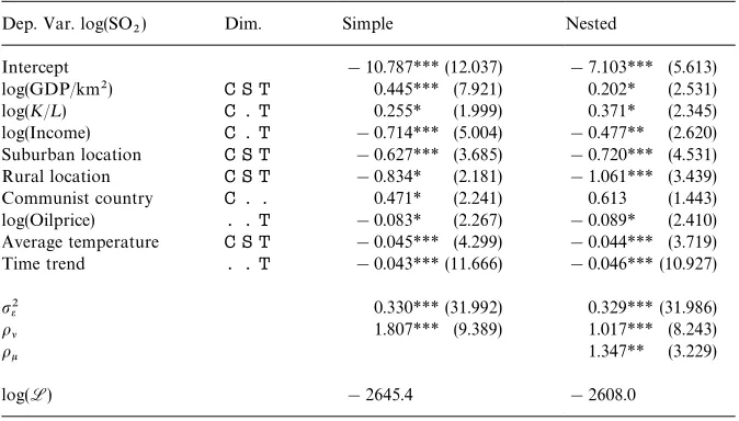
Table 1
Example regression: Simple vs. Nested! Dep. Var. log(SO
2) Dim. Simple Nested
Intercept !10.787***(12.037) !7.103*** (5.613)
log(GDP/km2) C S T 0.445*** (7.921) 0.202* (2.531)
log(K/¸) C . T 0.255* (1.999) 0.371* (2.345)
log(Income) C . T !0.714*** (5.004) !0.477** (2.620)
Suburban location C S T !0.627*** (3.685) !0.720*** (4.531)
Rural location C S T !0.834* (2.181) !1.061*** (3.439)
Communist country C . . 0.471* (2.241) 0.613 (1.443)
log(Oilprice) . . T !0.083* (2.267) !0.089* (2.410)
Average temperature C S T !0.045*** (4.299) !0.044*** (3.719)
Time trend . . T !0.043***(11.666) !0.046***(10.927)
p2e 0.330***(31.992) 0.329***(31.986)
ol 1.807*** (9.389) 1.017*** (8.243)
ok 1.347** (3.229)
log(L) !2645.4 !2608.0
!¹ratios are given in parenthesis. The second column indicates over which dimensions the variable varies:&C'indicates country,&S'indicates observation station, and&T'indicates time.
*Signi"cance at 95% con"dence level.
**Signi"cance at 99% con"dence level.
***Signi"cance at 99.9% con"dence level. 4. Empirical example
To illustrate the practical value of the method introduced in Section 3, Table 1 compares the estimates from a conventional non-nested random e!ects ML estimation with those from a nested-e!ects ML estimation.
The example is a constant-elasticity closed-economy version of the regression model in Antweiler et al. (1998). The original model passed a number of standard robustness and speci"cation checks. The dependent variable in this model is the log of atmospheric sulfuric dioxide concentration at observation stations around the world. A total of 2621 observations are obtained from 293 observation stations located in 44 countries, spanning a time period (not necessarily continuous) from 1971 to 1996. In this highly unbalanced panel, about a third of the observations are from stations in the United States. The second column in Table 1 indicates the dimensions of the independent variables. The indicators&C',&S', and&T' symbolize the dimensionscountry, observation
log of a country's capital abundance, and the log of its lagged 3-year moving income per capita. These regressors correspond (in that order) to the scale, composition, and technique e!ect that determine pollution concentration. Additional regressors are station-speci"c factors such as average temperature and the geographic proximity to urban centres (suburban and rural location dummies). A communist-country dummy, a time series for the real price of crude oil, and a time trend conclude the set of regressors for this model.
The results of this comparison shed some light on the problems with nested and highly unbalanced panels. First, the magnitudes of the estimates of the key regressors are noticeably di!erent across the two models. The scale elasticity is only one-half the value from the non-nested panel estimation, while the import-ance of the composition e!ect has increased, and the income e!ect has de-creased. While these results still (and strongly) support the conclusions in Antweiler et al. (1998), they cast doubt on the reliability of the point estimates. Second, the decomposition of the error term permits a clearer view on the aggregation level where the disturbances are introduced. In the simple model, the station and country variations are lumped together. When they are disag-gregated it appears that more variation is at the country level than at the station level. Third, insofar as the simple model can be viewed as being nested within the more general nested-panel model, a likelihood ratio test between the two models with a test statistic of 74.8 is highly signi"cant and favours the nested-panel model.
5. Monte-Carlo simulation
Comparing variance components estimators for unbalanced panel data re-quires comparison under a variety of panel patterns and true values of the variance components. An early Monte-Carlo study by Maddala and Mount (1973) evaluated the performance of di!erent estimators for panel data. A recent and very thorough study by Baltagi and Chang (1994) comes to the conclusion that the ML estimator performs better than ANOVA-type estimators in severely unbalanced panels and when variance component ratios are large. The Baltagi and Chang study also introduces important concepts for the design of a Monte-Carlo study for such unbalanced panels which I will follow in this section. Here I investigate the performance of the new ML estimator for a double-nested panel and compare its performance with the conventional non-nested random-e!ects ML estimator.
11The data generation process (DGP) is an adaptation from Nerlove (1971a); see also Baltagi et al. (1999b). Here,x
1,ijkt"0.2t#0.9x1,ijk,t~1wijt,x2,ijt"0.3t#0.8x2,ij,t~1#wij, andx3,it"0.3t #0.8x
3,ij,t~1#wi, where thewijk,wijandwiare uniformly distributed on the interval [!z,#z] with z equal to 0.5, 5, and 1, respectively. The initial observations are de"ned as
x
1,ijk0"4#2wij0,x2,ij0"40#20wij0, andx3,i0"8#5wi0. The truebis [10,3,0.2,!1.5]. Start-ing values for the ML routine are OLS estimates for the non-nested ML, and estimates from the non-nested ML were used in turn as starting values for the nested ML.
A generalization of this concept to nested panels is as follows:
ul,G/+Li/1+Mj/1i +Nk/1ij (1/¹ijk)
H/G , uk,
F/+Li/1+Mi
j/1(1/Nij)
G/F
uj,¸/+Li/1(1/Mi)
F/¸ .
I consider two degrees of unbalancedness: strong unbalancedness (;)
corre-sponds to a pattern of seven groups with M16, 11, 10, 7, 3, 1, 1N subgroups (implyingu"0.366), while weak unbalancedness (u) corresponds to a pattern of seven groups with a uniformM2,2,12Ndistribution of subgroups (implying an average ofu"0.827). In all cases, groups have an average of seven subgroups, which implies a sample size of H"74"2,401 observations. In varying the degree of unbalancedness over the three hierarchical levels in the panel, I con-sider the six patterns;uu,u;u,uu;,;;u, ;u;, andu;;.
The variance decomposition will be measured by the familiar ol, ok, and oj variance ratios, "xing p2e at 5. I consider 10 permutations of the variance ratios 0.1, 0.4, and 0.7 for each of the threeo's that satisfy 1!oj!o
k!ol'0. WithHandp2e "xed, the parameter space (ul,uk, uj, ol,ok,oj) encompasses 60 di!erent models. The Monte-Carlo simulation was conducted with 500 replications of each model, making use of the analytic gradient for the log-likelihood function documented in the appendix. The true model is assumed to be
y
ijkt"b0#b1x1,ijkt#b2x2,ijt#b3x3,it#ji#kij#lijk#eijt, (34)
withx
3varying only at the top (e.g., country) level,x2varying at the mid (e.g.,
province) level, andx
1available for all observations at the most detailed (e.g.,
city) level.11
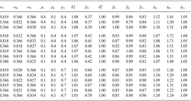
Results of the simulation are shown in Table 2. The"rst group (six columns) in the table identi"es the parameter space (suppressing the"xedHandp2e). The second group }consisting of the p(2e and o(
u columns} shows results for the
Table 2
Monte-Carlo simulation results
ul uk uj ol ok oj p(2e o(
u p(2e o(l o(k o(j sb1 sb2 sb3 0.819 0.819 0.366 0.1 0.1 0.1 1.01 0.28 1.00 0.88 0.89 0.69 1.10 1.25 1.11 0.819 0.366 0.827 0.1 0.1 0.1 1.01 0.29 1.00 0.90 0.85 0.73 1.10 1.27 1.16 0.366 0.821 0.823 0.1 0.1 0.1 1.01 0.28 1.00 0.89 0.88 0.70 1.10 1.22 1.10 0.819 0.366 0.366 0.1 0.1 0.1 1.01 0.25 1.00 0.95 0.86 0.62 1.11 1.30 1.11 0.366 0.822 0.366 0.1 0.1 0.1 1.01 0.28 1.00 0.83 0.89 0.69 1.09 1.22 1.09 0.366 0.366 0.826 0.1 0.1 0.1 1.01 0.30 1.00 0.86 0.90 0.70 1.10 1.25 1.10
0.820 0.819 0.366 0.4 0.1 0.1 1.08 0.15 1.00 0.99 0.78 0.60 1.13 1.36 1.08 0.819 0.366 0.822 0.4 0.1 0.1 1.08 0.16 1.00 1.00 0.74 0.69 1.12 1.40 1.09 0.366 0.820 0.826 0.4 0.1 0.1 1.08 0.16 1.00 0.99 0.83 0.64 1.10 1.30 1.07 0.819 0.366 0.366 0.4 0.1 0.1 1.08 0.15 1.00 0.99 0.79 0.56 1.13 1.39 1.12 0.366 0.821 0.366 0.4 0.1 0.1 1.08 0.17 1.00 1.00 0.76 0.63 1.10 1.29 1.07 0.366 0.366 0.825 0.4 0.1 0.1 1.08 0.17 1.00 0.99 0.79 0.62 1.12 1.31 1.09
0.820 0.822 0.366 0.7 0.1 0.1 1.22 0.12 1.00 0.99 0.79 0.55 1.06 1.43 1.04 0.819 0.366 0.824 0.7 0.1 0.1 1.22 0.12 1.00 0.99 0.74 0.58 1.07 1.43 1.03 0.366 0.820 0.827 0.7 0.1 0.1 1.22 0.12 1.00 0.99 0.83 0.57 1.03 1.29 1.00 0.819 0.366 0.366 0.7 0.1 0.1 1.22 0.12 1.00 1.00 0.75 0.58 1.07 1.44 1.05 0.366 0.820 0.366 0.7 0.1 0.1 1.22 0.14 1.00 1.00 0.88 0.50 1.04 1.29 1.02 0.366 0.366 0.825 0.7 0.1 0.1 1.22 0.13 1.00 1.00 0.77 0.62 1.04 1.29 1.01
0.819 0.819 0.366 0.1 0.4 0.1 1.07 0.33 1.00 0.91 0.97 0.51 1.09 1.78 1.11 0.819 0.366 0.832 0.1 0.4 0.1 1.06 0.30 1.00 0.91 0.97 0.54 1.09 1.72 1.07 0.366 0.818 0.827 0.1 0.4 0.1 1.07 0.27 1.00 0.87 0.98 0.55 1.07 1.50 1.06 0.819 0.366 0.366 0.1 0.4 0.1 1.07 0.27 1.00 0.91 0.97 0.50 1.08 1.74 1.08 0.366 0.819 0.366 0.1 0.4 0.1 1.07 0.33 1.00 0.85 0.98 0.60 1.07 1.51 1.05 0.366 0.366 0.827 0.1 0.4 0.1 1.06 0.32 1.00 0.89 0.98 0.63 1.07 1.48 1.05
0.818 0.817 0.366 0.4 0.4 0.1 1.13 0.21 1.00 0.99 0.97 0.52 1.10 1.66 1.06 0.818 0.366 0.825 0.4 0.4 0.1 1.13 0.20 1.00 1.00 0.96 0.65 1.10 1.65 1.03 0.366 0.819 0.822 0.4 0.4 0.1 1.13 0.18 1.00 0.99 0.97 0.61 1.08 1.47 1.05 0.820 0.366 0.366 0.4 0.4 0.1 1.13 0.19 1.00 0.99 0.96 0.57 1.09 1.72 1.05 0.366 0.821 0.366 0.4 0.4 0.1 1.13 0.22 1.00 1.00 0.97 0.59 1.08 1.47 1.05 0.366 0.366 0.824 0.4 0.4 0.1 1.13 0.21 1.00 1.00 0.95 0.59 1.10 1.47 1.06
0.819 0.819 0.366 0.1 0.7 0.1 1.19 0.36 1.00 0.87 0.97 0.71 0.98 1.69 0.94 0.819 0.366 0.825 0.1 0.7 0.1 1.17 0.30 1.00 0.87 0.97 0.69 1.00 1.67 0.97 0.366 0.819 0.833 0.1 0.7 0.1 1.19 0.26 1.00 0.89 0.97 0.63 0.97 1.43 0.95 0.819 0.366 0.366 0.1 0.7 0.1 1.19 0.29 1.00 0.94 0.98 0.61 0.97 1.69 0.95 0.366 0.818 0.366 0.1 0.7 0.1 1.19 0.34 1.00 0.86 0.98 0.65 0.96 1.43 0.95 0.366 0.366 0.823 0.1 0.7 0.1 1.17 0.31 1.00 0.92 0.97 0.62 0.98 1.41 0.96
0.819 0.821 0.366 0.1 0.1 0.4 1.01 0.58 1.00 0.89 0.88 0.87 1.10 1.25 1.09 0.819 0.366 0.828 0.1 0.1 0.4 1.01 0.57 1.00 0.82 0.88 0.86 1.10 1.28 1.08 0.366 0.818 0.827 0.1 0.1 0.4 1.01 0.60 1.00 0.92 0.87 0.89 1.10 1.22 1.09 0.819 0.366 0.366 0.1 0.1 0.4 1.01 0.57 1.00 0.91 0.85 0.85 1.10 1.28 1.08 0.366 0.819 0.366 0.1 0.1 0.4 1.01 0.60 1.00 0.87 0.86 0.89 1.09 1.22 1.09 0.366 0.366 0.824 0.1 0.1 0.4 1.01 0.57 1.00 0.88 0.90 0.85 1.10 1.24 1.09
Table 2 (continued)
ul uk uj ol ok oj p(2e o(
u p(2e o(l o(k o(j sb1 sb2 sb3 0.819 0.366 0.366 0.4 0.1 0.4 1.08 0.37 1.00 0.99 0.86 0.83 1.12 1.41 1.05 0.366 0.822 0.366 0.4 0.1 0.4 1.08 0.37 1.00 0.99 0.79 0.84 1.11 1.30 1.08 0.366 0.366 0.830 0.4 0.1 0.4 1.08 0.39 1.00 1.00 0.84 0.90 1.10 1.31 1.08
0.818 0.822 0.366 0.1 0.4 0.4 1.07 0.42 1.00 0.93 0.99 0.80 1.07 1.72 1.04 0.818 0.366 0.832 0.1 0.4 0.4 1.06 0.41 1.00 0.87 0.99 0.82 1.08 1.71 1.05 0.366 0.818 0.827 0.1 0.4 0.4 1.07 0.40 1.00 0.92 0.99 0.83 1.06 1.51 1.05 0.819 0.366 0.366 0.1 0.4 0.4 1.07 0.41 1.00 0.87 1.00 0.80 1.08 1.75 1.05 0.366 0.819 0.366 0.1 0.4 0.4 1.07 0.42 1.00 0.86 0.99 0.82 1.06 1.51 1.05 0.366 0.366 0.825 0.1 0.4 0.4 1.06 0.42 1.00 0.90 0.99 0.82 1.07 1.49 1.05
0.819 0.820 0.366 0.1 0.1 0.7 1.01 0.66 1.00 0.87 0.89 0.85 1.10 1.26 1.08 0.819 0.366 0.824 0.1 0.1 0.7 1.01 0.69 1.00 0.86 0.91 0.89 1.10 1.29 1.08 0.366 0.822 0.827 0.1 0.1 0.7 1.01 0.69 1.00 0.83 0.91 0.90 1.09 1.22 1.09 0.819 0.366 0.366 0.1 0.1 0.7 1.01 0.67 1.00 0.88 0.89 0.86 1.10 1.31 1.08 0.366 0.821 0.366 0.1 0.1 0.7 1.01 0.68 1.00 0.85 0.86 0.87 1.09 1.22 1.09 0.366 0.366 0.834 0.1 0.1 0.7 1.01 0.70 1.00 0.85 0.90 0.90 1.10 1.24 1.09
12There appears to be a downward bias in the estimates ofok, and more pronounced,oj. While this appears puzzling at"rst sight, closer inspection of the simulation results reveals that the estimates ofokandojare in some cases approaching zero, while in other cases, there are right on target. The average shown in the table re#ects the mixing of these cases. This peculiarity may be attributed to the high degree of non-linearity of the log-likelihood function (and its partial derivatives) which in turn may lead to numerical instability in the maximization routine.
variance; in the case ofo(
uthe ratio is relative tooj#ok#ol. The last group of
three columns shows the standard errors obtained for the parameter estimates b1, b2, andb3, where each is expressed as the ratio of the standard error from the nested-e!ects estimation relative to the standard error from the non-nested-e!ects estimation. For brevity, information on bias of the regressor estimates is not included as they were found to be negligible.
The Monte-Carlo simulation provides several interesting results. First, the use of the non-nested panel estimation for a nested panel does not deliver a clear picture of the variance decomposition. When estimating a nested model with the conventional non-nested random-e!ects ML estimator, p(2e is biased slightly upwards and ou"o
l#ok#oj is biased downwards. The bias seems to be more pronounced when the variance ratio ol is relatively large compared to ok andoj. The degree of unbalancedness only has a modest impact. Second, using the nested-e!ects estimator for a nested panel delivers much superior estimates of the variance terms.12 Third, the standard errors of parameter estimates obtained from the non-nested estimation appear to be biased. For the estimate of the standard error of b2 (corresponding to the variablex
2 which
theMoulton bias. This downward bias is persistent over the entire parameter space and is relevant for all three types of variables. The e!ect is noticeably pronounced in the case of b2 when eitherok orol are large, or when a large ok coincides with the corresponding panel level being highly unbalanced. In conclusion, the Monte-Carlo results suggest that inferences drawn from a non-nested estimation of a nested panel may be inaccurate because the standard errors are downward biased.
6. Conclusions
Hierarchically structured panel data are a common feature in many econo-metric studies. This paper has argued that a nested structure for the error term is a suitable way to deal with related pertinent econometric problems. In particu-lar, nested-e!ects models provide a method for addressing the problem of merging micro and macro data. This paper has focused on unbalanced panels, acknowledging their pervasiveness in applied work. The maximum-likelihood estimator introduced in this paper provides a convenient estimation method. The double-nested error structure discussed here also provides the basis for generalizations to higher-order nested error structures.
I have compared the performance of the double-nested ML estimator with the performance of the conventional non-nested ML estimator. The results from the corresponding Monte-Carlo simulation reveal a downward bias in the standard errors of the regressors when the conventional (non-nested) random-e!ects estimator is applied to a nested panel. This key"nding, along with illustrating the comparative performance of the estimator in a practical application, make a solid case for using the nested-e!ects ML estimator.
A caveat applies to the exclusion of separate time e!ects in this model. One way to deal with possible time e!ects is to introduce"xed time e!ects or a time trend variable. It appears that extending the present model to a `two-waya
model with random time e!ects is very challenging because the time e!ects and hierarchical individual e!ects overlap in a non-trivial manner.
The discussion of the nested-e!ects ML estimator in this paper is directed at applied econometricians. Researchers interested in using this estimator can obtain the software developed for this paper by sending an e-mail request to the author.
Acknowledgements
DiNardo and David Green for helpful comments. I am particularly grateful for the suggestions and comments from one very helpful anonymous referee. This project was supported, directly or indirectly, by grants from the Social Sciences and Humanities Research Council of Canada, UBC's Centre for International Business Studies, and UBC's Entrepreneurship and Venture Capital Research Centre.
Appendix. Derivation of+L
In what follows I derive the analytic gradient +L of the log-likelihood
function. The derivatives are highly non-linear. For notational convenience let
LL
wherebf is the estimate corresponding to thefth regressor in the model.
References
Ahrens, H., Pincus, R., 1981. On two measures of unbalancedness in a one-way model and their relation to e$ciency. Biometric Journal 23, 227}235.
Antweiler, W., Copeland, B., Taylor, M.S., 1998. Is free trade good for the environment? National Bureau of Economic Research Working Paper Seriesd6707. Forthcoming, American Economic Review.
Baltagi, B.H., 1987. On estimating from a more general time-series cum cross-section data structure. The American Economist 31, 69}71.
Baltagi, B.H., 1993. Nested e!ects (Problem 93.4.2). Econometric Theory 9, 687}688. Baltagi, B.H., 1995. Econometric Analysis of Panel Data. Wiley, Chichester, UK.
Baltagi, B.H., Chang, Y.-J., 1994. Incomplete panels: a comparative study of alternative estimators for the unbalanced one-way error component regression model. Journal of Econometrics 62 (2), 67}89.
Baltagi, B.H., Song, S.H., Jung, B.C., 1999a. Further evidence on the unbalanced two-way error component regression model. Discussion paper, Texas A&M University.
Baltagi, B.H., Song, S.H., Jung, B.C., 1999b. The unbalanced nested error component regression model. Discussion paper, Texas A&M University.
Davis, P., 1999. Estimating multi-way error components models with unbalanced data structures. Mimeo, MIT Sloan School.
Fuller, W.A., Battese, G.E., 1973. Transformations for estimation of linear models with nested error structures. Journal of the American Statistical Association 68 (343), 626}632.
Ghosh, S.G., 1976. Estimating from a more general time-series cum cross-section data structure. The American Economist 20, 15}21.
Hsiao, C., 1986. Analysis of Panel Data. Cambridge University Press, Cambridge, MA.
Maddala, G.S., Mount, T.D., 1973. A comparative study of alternative estimators for variance components models used in econometric applications. Journal of the American Statistical Association 68, 324}328.
Moulton, B.R., 1986. Random group e!ects and the precision of regression estimates. Journal of Econometrics 32, 385}397.
Moulton, B.R., 1987. Diagnostics for group e!ects in regression analysis. Journal of Business and Economic Statistics 5, 275}282.
Moulton, B.R., 1990. An illustration of a pitfall in estimating the e!ects of aggregate variables on micro units. Review of Economics and Statistics 72 (2), 334}338.
Nerlove, M., 1971b. A note on error components models. Econometrica 39, 383}396.
Pakes, A., 1983. On group e!ects and errors in variables in aggregation. Review of Economics and Statistics 65, 168}173.
Searle, S.R., 1987. Linear Models for Unbalanced Data. Wiley, New York.
Sydsvter, K., Str+m, A., Berck, P., 1999. Economists'Mathematical Manual, 3rd Edition. Springer, Berlin.
Wansbeek, T., Kapteyn, A., 1982. A class of decompositions of the variance}covariance matrix of a generalized error components model. Econometrica 50 (3), 713}724.
Wansbeek, T., Kapteyn, A., 1989. Estimation of the error-components model with incomplete panels. Journal of Econometrics 41, 341}361.