Cross-sectional aggregation of non-linear
models
Kees Jan van Garderen
!
, Kevin Lee
"
,
M. Hashem Pesaran
#,$,
*
!University of Bristol, UK
"University of Leicester, UK
#University of Cambridge, Faculty of Economics and Politics, Austin Robinson Building,
Sidgwick Avenue, Cambridge CB3 9DD, UK
$University of Southern California, USA
Abstract
This paper considers the problem of cross-sectional aggregation when the underlying micro behavioural relations are characterized by general non-linear speci"cations. It focuses on forecasting the aggregates, and shows how an optimal aggregate model can be derived by minimizing the mean squared prediction errors conditional on the aggregate information. The paper also derives model selection criteria for distinguishing between aggregate and disaggregate models when the primary object of the analysis is forecasting the aggregates, and establishes the consistency of the model selection criteria in large samples. In the case of standard non-linear micro relations with additive errors it also provides suitable small sample corrections. For more general non-linear speci"cations we consider bootstrap techniques to correct for small sample bias of the proposed model selection criteria. Some of the ideas in the paper are illustrated using log-linear micro relations, often employed in applied research. The paper also contains an empirical application where log-linear production functions are estimated for the UK economy disaggregated by eight industrial sectors and at the aggregate level over the period 1954}1995. ( 2000 Elsevier Science S.A. All rights reserved.
JEL classixcation: C43; C52; E23
*Corresponding author. Tel.:#44-1223-335-216; fax:#44-1223-335-471.
E-mail address:[email protected] (M.H. Pesaran)
Keywords: Aggregation; Prediction; Model selection; Non-linear models; Log-linear speci"cations; Production functions; Parametric bootstrap
1. Introduction
Recently there has been a renewal of interest in the aggregation problem, partly due to the increased availability of panel data sets which cover a large number of micro units (such as households,"rms, industries, or regions) over relatively long periods of time, and partly due to the signi"cant advances made in computations. Under the in#uence of the seminal contributions of Gorman (1953), Klein (1953, Chapter 8), Theil (1954), Grunfeld and Griliches (1960), and Ando (1971), the literature on aggregation has focussed on two separate but closely related issues; namely the&aggregation problem', and the&model selec-tion problem'. The former literature attempts to derive conditions under which macro models will re#ect and provide interpretable information on the underly-ing behaviour of the micro units (households and"rms).1The latter literature is concerned with the problem of choosing between the aggregate and the disag-gregate speci"cations when the object of interest is prediction of the aggregate (or macro) phenomena. Early work in this area has been more recently extended by Pesaran et al. (1989) (PPK) and Pesaran et al. (1994) (PPL) where selection criteria are proposed which are appropriate for choosing between linear aggre-gate and disaggreaggre-gate models based on prediction of the aggreaggre-gate variables in di!erent contexts.
This paper is concerned with some of the implications of aggregation when the underlying micro relations are non-linear. The aggregation problem is particularly complicated in the presence of non-linearities and does not lend itself to a satisfactory solution, except under very stringent conditions on the form of the non-linearity and/or the nature of the heterogeneity in the behav-ioural relations across the micro units. The model selection problem is also di$cult to deal with, especially when the micro relations involve dynamics as well as non-linearities. Consequently, the analysis of the model selection prob-lem has typically focussed on linear disaggregate models, despite the fact that many, and perhaps most, empirical applications involve important non-lineari-ties due to the log-linear form of the micro-relations often favoured by applied researchers.
The focus of this paper is primarily on the model selection problem and provides a theoretical basis for comparisons of predictions of the aggregate variables based on the aggregate and disaggregate models, taking proper ac-count of the di!erent information sets that are applicable to the two sets of predictions. We derive consistent model selection criteria, in the sense that their use results in the selection of the correct model asymptotically. This analysis has parallels with the&forecasting approach'to the aggregation problem proposed in Pesaran (1999), where the aggregate model is derived as conditional optimal forecasts of the aggregates based on a given disaggregate speci"cation. The focus of this approach is on predictions of the aggregate variables, and derives the optimal aggregate model by minimizing the mean squared prediction errors conditional on the &aggregate', or the publicly available information. The ap-proach is applicable irrespective of whether the disaggregated model is linear, non-linear or involves dynamics. This paper, however, abstracts from dynamics, but deals with general non-linear speci"cations. The proposed non-linear ag-gregation method will be illustrated in the context of log-linear micro relations, widely employed in empirical analysis. This application emphasizes the useful-ness of the approach, by setting out explicitly the functional form that should be estimated for a macro model when the underlying micro relationships are log-linear. It will be shown that even in the case of this simple model, in general, it is not possible to identify the parameters of the micro relations from those of the optimal aggregate function. Furthermore, in the case where the slope coe$cients are allowed to di!er across the micro relations the optimal aggregate speci"cation will generally involve squares and cross-products of the logarithms of the aggregate variables even though the underlying micro relations are assumed to be log-linear.
The use of model selection criteria in discriminating between aggregate and disaggregate models also provides insights into possible mis-speci"cation of the disaggregate model. The association between model selection criteria and mis-speci"cation tests in the context of linear disaggregate models has been dis-cussed in PPK and PPL. For a general treatment of model selection and mis-speci"cation analysis see, for example, White (1994).
Even though the proposed model selection criterion is asymptotically
industrial sectors in the UK economy using annual observations over the period 1954}1995.
The plan of the paper is as follows: Section 2 sets out the disaggregate model, introduces the necessary notations, provides a brief overview of the alternative approaches to the aggregation problem that have been con-sidered in the literature, and argues in favour of the &forecasting approach'. Section 3 discusses the form of the choice criteria to be used in comparing micro and macro models in terms of their ability to predict macro variables and describes how these criteria can be used in testing for model mis-speci"cation. Section 4 illustrates the approach of the paper by means a number of simple examples, primarily focussing on the problem of the optimal aggregation of log-linear micro relations typically employed in applied research. Section 5 pres-ents the empirical application. Finally, some concluding remarks are provided in Section 6.
2. Prediction and aggregation
2.1. Formulation of the problem
Suppose there areNmicro units (such as individuals,"rms, industries, sectors, regions) indexed by i whose decision variable, >
it, is observed over ¹ time
periods. Further, assume that these decision variables are set according to the following non-linear relations:
H
$: >it"n(Xit, hi, eit), i"1, 2,2,N; t"1, 2,2,¹, (2.1)
where n()) is a function, which could be continuous or discrete, Xit"
(X(1)
it , X(2)it ,2, X(itk))@, are k]1 vectors of explanatory variables, hi is a p]1
vector of unknown parameters speci"c to the micro unit, ande
itis a disturbance
term.2 Aggregate e!ects that are common across micro units can also be included inX
it.3In this paper, we con"ne our analysis to the case whereXit's
are strictly exogenous and assume that neither lagged values of>
itnor
contem-poraneous values of>
jt,jOi, are included among the explanatory variables,Xit.
Accordingly, we assume:
2Note that Eq. (2.1) allows for parameter heterogeneity across micro units as well as the heterogeneity of inputs, X
it, across i. In the special case where p()) is linear, only parameter
heterogeneity can result in aggregation problems.
Assumption 2.1. The error terms, e
it, have distribution functions containing
a"nite number of parameters denoted byu
i, and are distributed independently
ofX
iqandhi for all values ofi, tandq.
Throughout, the focus of the analysis will be on prediction of the aggregate variable,>
t"+Ni/1>it, whereNis"nite. The analysis is readily extended to the
case where the aggregate is de"ned more generally as averages or weighted averages across the decision variables of the micro units, so long as the weights are "xed and do not vary with ¹ or other parameters of the model. The disaggregate speci"cations given by (2.1) clearly provide a valid basis for prediction of the aggregates >
t. But it could be highly data intensive and
computationally very costly to work with, particularly when N is relatively large.4 In practice it could also be the case that the disaggregate model may be incorrectly speci"ed, or its explanatory variables may be subject to measurement errors, a problem which could become less serious as a result of cross-sectional aggregation (see, for example, Aigner and Gold"eld, 1974). It is therefore worth considering aggregate models that directly focus on,
>
t, the variable of interest. In what follows we shall consider alternative ways
that this can be done. However, in general an arbitrary aggregate model can be written as
H
': >t"g(Zt,d)#vt, t"1, 2,2,¹, (2.2)
where d is a p
g]1 vector of unknown parameters, E(vtDZt)"0,Zt is a
k
g]1 vector of explanatory variables, which will typically include the
ag-gregatesX
t"+Ni/1Xit, as well as the lagged values of >t and other aggregate
variables which may not have a micro counterpart in the disaggregated
speci-"cations. In the case where the functional form of the micro equations is the same across the micro units, the aggregate model is often speci"ed as the analogue of the micro equations withX
tsubstituted for the micro variables,
X
itThe aggregation problem is concerned with the relationship (if any) between.
the parameters of the micro equations in (2.1), and those of the macro equation in (2.2). Traditional approaches to this problem have focused on whether there exists an aggregate model, based on aggregate variables only, which can provide information with which to identify the parameters of the micro behavioral model de"ned by (2.1). Within this tradition, a &deterministic approach' is observed in the literature, in which the error termse
itare set equal to zero, and
the aggregation is then carried out conditional on given values ofX
itandhi. The
central issue in this approach has been to obtain conditions under which the
aggregation of the micro equations results in an aggregate model with para-meters that provide direct measures of the underlying micro parapara-meters,h
i.5
These conditions turn out to be extremely restrictive and are unlikely to hold in practice. More recently, a &stochastic approach' to aggregation has also been advanced by Kelejian (1980) and Stoker (1984, 1986) in which the heterogeneity across the micro relations is modelled as a joint probability distribution func-tion over (X
it, hi, eit) with a"nite number of parameters, and then the aggregate
model is derived as relationships between theunconditional "rst, and possibly higher-order, moments of>
itand Xit. Utilizing this approach, Stoker
demon-strates that, even if there is no parameter heterogeneity across the micro relations, the parameters of the marginal distribution of theX
itwill generally
enter the aggregate model when the underlying micro relations are non-linear. This in turn means that cross-sectional aggregation of non-linear relations is not generally invariant to changes in the composition of X
itover time. In these
circumstances, parameter estimates of the macro model will be a composite of the micro parameters and the distributional parameters of the explanatory variables of the model.6
Both the deterministic and the stochastic approaches to aggregation are aimed at the problem of how to recover behavioural micro parameters from the estimates of the macro model, and how to formulate a macro model so that such a recovery process is in fact feasible. Unfortunately, the aggregation problem, as traditionally formulated, is resolved only under very stringent conditions, rarely applicable in practice. Consequently, the traditional analysis of the aggregation problem generally is not very useful in data analysis. The stringency of the conditions under which micro and macro parameters can be related has also led many macro economist either to ignore the aggregation problem altogether, or to undermine its importance by appealing to the &representative agent' para-digm.7
5Gorman's (1953) work on linear Engel curves provides a good illustration of this approach, in which attention focuses on the form off()) withXit"Xt"Ztandhi"hfor alli. Muellbauer (1975)
discussion of&generalised linearity'illustrates the possibility that attention might also focus on the de"nition of the aggregate variable,Z
t, as well as on the form off()).
6The stochastic approach is also employed in the context of log-linear models by Lewbel (1989, 1992). Assuming that there is no parameter heterogeneity, Lewbel shows that a &mean scaling'
condition on the distribution ofX
itprovides the necessary and su$cient restrictions for identi"
ca-tion of the micro parameters from the estimates of the parameters of the analogue macro relaca-tion. Without such a condition, aggregation will still be a problem even in this relatively simple model.
2.2. A forecasting approach to the aggregation problem
An alternative approach, applied in Pesaran (1999) to the analysis of aggrega-tion in linear dynamic models, focuses on the predicaggrega-tion problem as the primary objective and derives the aggregate model as a conditional optimal forecast (in the minimum mean squared error sense) of >
t, taking the micro relations as
given.8Di!erent aggregate functions are obtained depending on the nature of the information set used in the forecasting exercise. Here we consider the application of the forecasting approach to the non-linear micro relations in (2.1) under di!erent information sets. In particular, we shall consider the following information sets:
U
it: the micro information set specitaining current and lagged values of"c to theX ith micro unit, con-it,
W
t: the aggregate information set common to all micro units,containing the current and lagged values of the aggregate
variables, including those ofX
t,
X
it"UitXWt: the information set available to theith micro unit,
X
t"6Ni/1Xit: the universal information set, containing current and laggedvalues ofX it, fori"1, 2,2,N.
Di!erent optimal predictors of the aggregate variable,>
t, can now be derived
with respect to di!erent information sets. For this purpose we need the following assumption:
Assumption 2.2. The variables (>
1t, >2t,2, >Nt) are measurable with respect to
the non-decreasing information setsW
t,XitandXt, and have"nite second-order
moments both conditionally and unconditionally.
This assumption in particular ensures that the conditional expectations E[n(X
it, hi, eit)DXit,hi], E[n(Xit,hi, eit)DXit] exist and are"nite for alliandt.
The optimal disaggregate predictor of>
t, denoted by>$t, can now be written
as
>$
t"E[>tDXt]" N
+
i/1
E[>
itDXt]. (2.3)
Since interactions across micro units have been ruled out by assumption, so that the decision variable of theith micro unit is not a!ected by the forcing variables
of thejth micro unit (jOi), under Assumptions 2.1 and 2.2 we have
Therefore, when disaggregate information is available the optimal forecast of the aggregate can be computed by "rst forecasting the decision variable of the individual micro units and then aggregating the resultant forecasts.
For future purposes, it is also worth noting that
>
it"f(Xit, hi,ui)#mit, (2.6)
where, by construction (and under Assumption 2.2), we have E(m
itDXit)"0.
Similarly, for the aggregate errors,m
t"+Ni/1mit, we have E(mtDXt)"0. Hence,
both the disaggregate and aggregate errors are martingale di!erence processes with zero means and "nite variances. But, in general, mit and mt could be heteroskedastic both conditionally and unconditionally.
Suppose now we wish to forecast the aggregate variable of interest,>
t, but
only with respect to the aggregate information set,W
t. This could be due to the
absence of reliable micro observations and/or high costs of data processing and computations. In this case since, in general, individual micro parameters, h
i,
cannot be estimated, we derive the aggregate forecasts under the following assumption:
Assumption 2.3. The micro parameters,t
i"(h@i,u@i)@are randomly distributed
means and a positive de"nite variance covariance matrix.
This is the standard random coe$cient model utilized extensively in the litera-ture on heterogeneous panel data models. Under Assumptions 2.1}2.3, the optimal aggregate forecast, which we denote by>!
t, exists and is given by
In general, the derivation of E[n(X
it, hi,eit)DWt]"E[f(Xit, ti)DWt] can be quite
Furthermore, E[n(X
it, hi,eit)DXt] will depend on all the parameters of the joint
probability distribution of (X
it, hi, eit) conditional on Xt, which could be time
varying. Generally, therefore, the use of>!
t as a forecast of>twill not be feasible
without disaggregate information on the time evolution of the cross-sectional distribution ofX
it. The derivation of a feasible model for>!t, based on a"nite
number of parameters, will typically require further assumptions on the nature of theX
itprocess. To this end, a number of di!erent assumptions have been used
in the literature. For example, writingj
it"(X(1)it /X(1)t ,X(2)it /X(2)t ,2, X(itk)/X(tk))@,
i"1, 2,2, N, the&Hicks'aggregation condition'takesjitas being"xed over time. Lewbel (1992) considers a weaker version of the Hicks' condition and allowsjitto be time varying but requires that they are distributed independently ofX
t; this is known as the&scale invariant condition'. We adopt a more general
version of this assumption:
Assumption 2.4. The time evolution of the cross-sectional distribution ofj
itis
stationary, andj
itis distributed independently of the scale variableXt, for all
iandt.
Given the above assumptions, an optimal aggregate model containing a"nite number of parameters can be obtained.
Proposition 2.1. Suppose the decisionvariables,>
it,at the level of the micro units
i"1, 2,2, N, are set according to relations (2.1). Then, under Assumptions
2.1}2.4, the optimal aggregate model can be written as
>
t"h(Xt,c)#ut, (2.9)
where
E(u
tDXt)"0,<ar(utDXt)(R.
The optimal aggregate forecast is given by
>!
t"h(Xt, c)" N
+
i/1
E[p(j
it"Xt, hi, eit)DWt], "+N
i/1
E[f(j
it"Xt,ti)DXt], (2.10)
wherejit"Xtrepresents element-by-element multiplications of thevectorsjitandXt,
andcis axnite-dimensionalvector of unknown parameters of the joint distribution
of(jit,hi, eit).
Clearly there exists some relationship between c, the parameters of the optimal aggregate predictor function,h(X
t, c), and the parameters of the
cross-sectional distribution of the underlying micro coe$cients. In particular,c de-pends onh, the mean values of the micro coe$cients h
i. But, in general this
relationship is complex and does not allow identi"cation of all the components ofh(oru) fromc.
2.3. Optimality properties of alternative forecasts
Intuitively one would expect that optimal predictions of>
t based on
disag-gregated information to be at least as good as predictions that are based only on the aggregate information. If the disaggregate predictions were worse, we could aggregate the information to obtain the same predictions as those based on the aggregate information alone. This result, in fact, follows immedi-ately from the properties of optimal forecasts under quadratic loss and noting thatW
tLXt.
Proposition 2.2. Consider the aggregate forecasts>$
t and>!t,based on the
disag-gregate and agdisag-gregate information sets,X
tandWt,and dexned by (2.4) and (2.10),
respectively. Then under Assumptions 2.1}2.4
E(>
t!>$t)2)E(>t!>!t)2. (2.11)
Therefore, if reliable disaggregate information is available, it should be utilized in forecasting, even if the primary objective is to forecast the aggregate variables. The only exception is when the prediction of>
tbased on the aggregate
informa-tion is identical to the predicinforma-tion based on the universal informainforma-tion set. We de"ne this property as theperfect aggregation condition:
Dexnition 2.1 (Perfect aggregation condition).
>$
t">!t for allt (2.12)
where >$
t and >!t are the aggregate forecasts based on the universal and the
aggregate information sets, respectively. See (2.4) and (2.10).
The perfect aggregation condition implies that some of the disaggregate in-formation is not necessary for forecasting the aggregates (so that aggregation is a valid data reduction).
the forecast based on the general aggregate model, >'
t"g(Zt,d), is the same
as the optimal aggregate forecast, >!
t. The above results can now be
sum-marized as:
Proposition 2.3. Under Assumptions 2.1}2.4,the aggregate predictors>$
t,>!t,and
>'
t dexned using (2.4), (2.10), and (2.2), respectively,satisfy the optimality
prop-erty:
E(>
t!>$t)2)E(>t!>t!)2)E(>t!>'t)2. (2.13)
The equality signs hold if and only if all the three aggregate forecasts are equal.
The usefulness of the forecasting approach is illustrated in Section 4, where two relatively simple examples of non-linear aggregation is considered. Sec-tion 5 applies the approach to log-linear speci"cations of output in the UK, disaggregated by eight industrial sectors over the period 1954}1994. First, however, we consider the problem of selecting between the alternative aggregate forecasts when the underlying parameters are unknown.
3. Prediction and model selection
The ranking of the aggregate forecasts >$
t, >!t, and >'t in Proposition 2.3
assumes that the disaggregate model is correctly speci"ed and that the values of hi,u
i,c, anddare known. In this section, we relax the latter assumption and
consider model selection criteria that take account of the sampling variations when the unknown parameters of the forecasting equations are replaced by suitable estimates. It is worth noting that, due to the particular relationship that exits between the disaggregate and the aggregate models under consideration, a straightforward application of standard model selection procedures such as Akaike's information or Schwarz's Bayesian criteria is not possible. First the log-likelihood function of the aggregates>
tunder the disaggregate model,H$,
depends on all the micro parametersw"(t@
1,t@2,2,t@N)@ and the maximum
likelihood estimation of w based on such a log-likelihood function will still require information on the disaggregated observations and may not be feasible whenNis relatively large. Even ifNis small enough so that such a maximum likelihood estimation can be implemented, the resultant estimates will not be e$cient as compared to the ML estimates based on the disaggregated relations. But if, in comparison of the aggregate and the disaggregate models, the ML estimates of t
i based on the disaggregated model are used, the usual penalty
log-likelihood function of the aggregate model is penalized. A more direct approach is required.
Here we begin by establishing certain asymptotic results for selecting between aggregate predictions based on disaggregate and aggregate models using the mean squared prediction errors as our criteria. In particular, we consider
S2$"1
These relations are obtained from (2.4), (2.10) and(2.2), respectively, after replac-ing the unknown parameters by their estimates, denoted here by a hat. The estimatestKi, i"1, 2,2,N, are obtained using the disaggregate observations, whilec( anddK are computed using the aggregate observations only.
In what follows, it will be assumed that the non-linear predictor functions
f(X
it, ti),h(Xt,c) andg(Zt, d) can be readily computed for given values of the
parameters and the regressors. In most applications of interest, it may not be possible to obtain closed-form expressions forf(X
it, ti)"E[p(Xit,hi,eit)DXit,hi]
and h(X
t, c)"+Ni/1E[p(jitXt,hi, eit)DWt]. Nevertheless, these conditional
ex-pectations can be computed by stochastic simulation as in Brown and Mariano (1984, 1989), for example. This does not fundamentally change the results that follow. The assumption that the various predictor functions can be readily computed is therefore not very restrictive.
Finally, we need the following assumptions regarding the aggregate errors, m
tde"ned by (2.6), and the rates of convergence of the parameter estimates and
certain cross-product matrices (closely related to the variance matrices of the various estimators):
Assumption 3.1. The aggregate disturbances,mt"+Ni
/1mit, wheremitis de"ned
by (2.6), satisfy the condition
Assumption 3.2. The parameter estimates of the disaggregated model, wK"
where the pseudo-true values cH"c(w0), dH"d(w0) are, respectively, de"ned underH
Similarly,9 Assumption 3.1 imposes certain regularity conditions on the implied aggre-gate disturbances,m
t. Noting thatdt"m2t !E(m2t DXt) is a martingale di!erence
process, then (3.2) is satis"ed if d
t,t"1, 2,2, have bounded second-order
moments and m
t,t"1, 2,2 have bounded conditional variances.10 Whenmt
(or its micro components,m
it) are conditionally heteroskedastic, further
restric-tions on the moments of X
it and eit will also be required for (3.2) to hold.
Assumption 3.2 states that the parameter estimates (for the disaggregate and aggregate models) converge to their true or pseudo-true values at rates which could di!er from the usualJ¹convergence, and speci"es the exact dependence of the pseudo-true values, cHand dH, onw0, the true parameter values under the disaggregate model. Assumption 3.3 in e!ect speci"es the rate at which the variances of the various estimators should tend to zero. Both assumptions are satis"ed withq"1 in the case of standard non-linear regression models typi-cally analysed in the econometrics literature. See, for example, Jennrich (1969), Malinvaud (1970), White and Domowitz (1984), Amemiya (1985), Andrews (1987), and Gallant and White (1988). For a recent comprehensive text book treatment see Davidson and MacKinnon (1993, Chapter 5).
3.1. Asymptotic justixcation
Given the above assumptions we are now able to state the following theorem which provides a justi"cation for the use of the selection criteria, at least in large samples.
9If the rates of convergence for di!erent components of the estimators are not the same, we can partition the estimators in groups with the same rate of convergence and partitionQ
T(w0),QT(cH)
andQ
T(dH), accordingly. 10Notice that E(d
tDXt)"0, and thereforedtis a martingale di!erence sequence. If it is further
assumed that E(d2t)(*(R, it then follows from the law of large numbers for martingale di!erence sequences due to Chow (see Theorem 3.77 in White (1984, p. 58), for example) that
Theorem 3.1. Under Assumptions 2.1}2.4, and Assumptions 3.1}3.3, and assuming
that the parametervectorsw,canddarexnite dimensional, we have
plim
Thexrst inequality is strict if and only if
plim
The second inequality is strict if and only if
plim
When (3.12) and (3.13) are satis"ed, the inequalities in (3.11) will be strict and can be stated as
Hence, when the disaggregated speci"cationH
$, described in (2.1), is correct, the
choice criteria based on mean squared prediction errors ranks the di!erent models correctly in large samples. In the case where the perfect aggregation condition holds, the optimal aggregate model yields the same predictions as the disaggregate model and the two speci"cations are equivalent as far as the prediction of the aggregates are concerned.11If only aggregate information is available, then the mean squared prediction errors is smallest for the optimal aggregate model. These results hold under relatively weak assumptions. For example, it is not required that the structural disturbances,e
it, be distributed
independently across micro units.
In"nite samples, however, models may be incorrectly ranked due to stochas-tic variation and possible small sample biases in the estimation of the unknown parameters. We shall now consider two alternative methods of adjusting the mean squared prediction error criteria for such small sample biases.
3.2. Small sample adjustments
One possible approach to correcting for the small sample bias of the selection criteria is to adjustS2$(wK),S2!(c() andS2'(dK) by taking account of the higher-order
terms in their Taylor series expansions around the true or the pseudo-true valuesw0,cH, anddH, respectively. This is in e!ect the approach followed in PPK and PPL in the case of linear micro relations. Application of this procedure to the general non-linear micro speci"cations (2.1) is possible, but is rather com-plicated and requires further assumptions concerning the asymptotic distribu-tion of the parameter estimates, and will not be pursued in this paper. The problem, however, is much more manageable in the case where the disturbances, e
it, enter the micro relations additively, namely when the micro relations are
speci"ed as standard non-linear regression models typically analyzed in the literature:
>
it"f(Xit, hi)#eit, i"1, 2,2,N, (3.14)
where for eachi,eit1iid(0, p2i). For this formulation>
itis predicted optimally
with respect toX
itbyf(Xit, hi), which does not depend on the parameters of the
error process,e
it.
Under standard regularity conditions applicable to non-linear regression models we have:12
e(
i"Mi(h0i)ei#O1(¹~1@2), (3.15)
wheree(
iis the¹]1 vector of residuals for theith micro relation with its typical
element given bye(
it">it!f(Xit, hKi),e(i"(e(i1,e(i2,2, e(iT)@,
M
i(h0i)"IT!F0i(F0{i F0i)~1F0{i "IT!A0i, (3.16)
in which F0
i"(F0i1,F0i2,2, F0iT)@ is a ¹]pi matrix of the derivatives F0it"
Rf(X
it,h0i)/Rhi,t"1, 2,2,¹.13Similarly, for the optimal aggregate speci"cation
(2.9), we have
u("f#M0
xe#O1(¹~1@2), (3.17)
where u("(u(
1,u(2,2, u(T)@, u(t">t!h(Xt, c(), f"(f1, f2,2, fT)@, ft"
+Ni/1f(X
it,h0i)!h(Xt, cH),
MH
X"IT!HH(HH@HH)~1HH@"IT!AHX, (3.18)
HH"(HH1,H2H,2, HHT)@, and HHt"Rh(Xt, cH)/Rc. Notice that HH is a ¹]p! matrix,p
!being the dimension ofc.
12See, for example, Davidson and MacKinnon (1993, Section 5.6).
13Here by allowingp
ito di!er acrossi, we allow for the possibility that the parameters of the
Using (3.15) and (3.17), and following an analogous line of reasoning as in PPK, it is now possible to derive adjusted mean squared prediction errors for the disaggre-gate and the optimal aggredisaggre-gate models. For the disaggredisaggre-gate model, we have
SI2$"+N
i/1
N
+
j/1
p(
ij, (3.19)
where
p(
ij"(¹!pi!pj#Tr(AK iAKj))~1e(@ie(j, (3.20)
andAK
iis the estimate ofA0i obtained by evaluating it ath0i"hKi. For the optimal
aggregate model, the relevant corrected criterion is given by the familiar expression,
SI2!"u(@u(/(¹!p
!). (3.21)
A similar correction can also be applied to the mean squared prediction errors of the general aggregate model, (2.2).
3.2.1. Small sample corrections by parametric bootstraps
Even when the above corrections are possible, the small sample properties of
SI2$ and SI2! are not known. We propose an alternative parametric bootstrap procedure which is computer intensive but is more generally applicable. The approach could also have better small sample properties than the adjusted criteria, although at this stage this is a pure conjecture. Because the exact small sample distribution is not tractable given the non-linearities involved, we will simulate the distribution of the di!erence between the (unadjusted) choice criteria, where the di!erences are de"ned by
D
!$"S2!!S2$, D
'!"S2'!S2!, D
'$"S2'!S2$.
Asymptotically, we expectD
!$*0 if the model is correctly speci"ed, and we
would also expectD
'!*0 if the aggregation assumptions are correct. However,
in"nite samples, either of these statistics might be smaller than zero and it is not reasonable, therefore, to dispense with the disaggregate model simply because
D!$(0. Hence, instead of 0 we propose to use a valuedH!$(a) determined from the empirical distribution ofD
!$generated using bootstrap techniques such that
the probability of selecting the disaggregate model when it is correct is (1!a). In order to generate the simulated distribution of D
!$, D'!, and D'$, we use
a parametric bootstrap procedure which can be described as follows:
1. Estimate the disaggregate model, the optimal aggregate model, alternative aggregate model(s), and calculateS2$, S2!, S2', and their di!erencesD
!$,D'!,
2a. Simulate (bootstrap) observations on >
it under the disaggregate model,
using the estimateshKi.
2b. Calculate the selection criteriaS2$, S2!,S2', and their di!erencesD
!$,D'!, and D
'$using the simulated data.
3. Repeat the computations in Step 2 R times and construct the empirical (simulated) distribution ofD
!$,D'$, andD'!and determinedH!$(a),dH'$(a) and dH'!(a) from the information on the left tails of these distributions.
4. Compare the actual observed values (from step1) ofD
!$andD'!withdH!$(a)
anddH'!(a).
Simulations in Step 2 can be carried out either parametrically assuming a par-ticular probability density function for the errors, or non-parametrically.14Here we describe the details assuming the disturbances,e
it, are normally distributed.
We simulate ¹ observations across the N micro units, for every replication
r"1, 2,2, R. For therth replication we obtain a set of¹draws, denoted by et(r)"(e(1rt),e(2r)t,2,e(Ntr))@ for t"1, 2,2,¹, from a multivariate N(0,RK) distribu-tion, whereRK is the estimated variance covariance matrix of the disturbance terms, which allows for possible contemporaneous error correlations across micro relations. These are substituted, together with the estimated parameter valueshKi, in the micro relation (1) to obtain simulated values of>
it:
>(r)
it"f(Xit,hKi, e(itr)), i"1, 2,2, N; t"1, 2,2,¹; r"1, 2,2, R.
The corresponding aggregate values are computed as >(r)
t "+Ni/1>(itr). Using
these simulated observations, we can reestimate the model and calculate the selection criteria for each replication and each of the alternative models to obtainD(!$r)"S2(r)
! !S2($r), D('$r)"S2('r)!S2($r)andD('!r)"S2('r)!S2(!r),r"1, 2,2,R,
for use in Step 3.
In implementing Step 4, we adopt a strategy in which the disaggregate model is selected in preference to either aggregate model ifD
!$'dH!$(a) andD'$'dH'$,
otherwise, the aggregate model with the smallest mean squared prediction error is selected. This selection strategy treats the models asymmetrically, taking the disaggregate model as the maintained hypothesis, and abandoning it only if its in-sample predictive performance is unreasonably poor relative to the aggregate models. In this sense, the model selection strategy can be seen as a misspeci" ca-tion test of the disaggregate model. IfD!$(dH!$(a) orD'$(dH'$(a), then this can be considered as evidence with which to reject the disaggregated model. When this happens, the optimality ofH
!in (2.10) cannot be justi"ed with reference to
the disaggregate model, and selection from the aggregate models is based on predictive performance only.
4. Two illustrative examples
In this section, we illustrate the&forecasting approach'by applying it to two simple examples, namely quadratic and log-linear micro relations. In these examples we consider the aggregation problem when the micro parameters are homogeneous, as well as when they are heterogeneous across the micro rela-tions.
4.1. Cross-sectional aggregation of quadratic models
Consider the following simple example
>
it"a#bXit#cX2it#eit, eit&IN(0, p2). (4.1)
where the micro decision variable, >
it, is a quadratic function of the scalar
explanatory variable,X
it. Initially, we assume that the micro parameters are the
same acrossi.15Aggregating relations (4.1) we have
>
t"aN#bXt#c N
+
i/1 X2
it#et.
Under the stationary scale-invariance Assumption 2.4, we have X
it"jitXt,
whereX
t"+Ni/1Xit,jitare distributed independently ofXt, and have a
station-ary distribution with the constant means and variances,k
ijandp2ij. Therefore,
the optimal aggregate predictor function based on the aggregate information set,W
t, is given by
E[>
tDWt]"E[>tDXt]
"aN#bX
t#cX2t
A
EC
N+
i/1
j2
itDXt
DB
,"aN#bX
t#
C
c N+
i/1
(p2
ij#k2ij)
D
X2t.This implies the following optimal aggregate speci"cation
>
t"aN#bXt#
C
c N+
i/1
(p2
ij#k2ij)
D
X2t#ut, (4.2)where by construction E(u
tDXt)"0. Hence, consistent estimates of the micro
parameters,aandbcan be obtained using aggregate observations>
tandXt,
but without further information on cross-sectional distribution ofj
it, it will not
be possible to estimate c from the aggregate model. The estimate of the coe$cient of X2
t in the aggregate speci"cation yields a consistent estimate of
c+Ni/1(p2
ij#k2ij), which involves the means and variances of the share variables,
j
it.Suppose now the parameters of (4.1) vary across the micro relations according
to the following random coe$cient model (also see Assumption 2.3):
a
i"a#tia; bi"b#tib; ci"c#tic,
wheret
i"(tia, tib,tic)@ 1ID(0,Rt), is distributed independently of eitandXit. The optimal aggregate model in this more general case has exactly the same form as (4.2), but its disturbances,u
t, will now be conditionally heteroskedastic.
In particular we have
<(u
tDXt)"a0#a1X2t,
wherea
0'0 and a1'0 are functions of the variances and the covariances of
the (e
it,jit, ti). Once again only the means ofaiandbican be identi"ed from the
aggregate model.
4.2. Cross-sectional aggregation of log-linear models
Consider now the following log linear relations:
ln>
it"a#b@lnXit#eit, eit&IN(0,p2) fori"1, 2,2,N, (4.3)
where X
it and b are k]1 dimensional vectors. Let git"log(jit)"
log(X
it)!log(Xt)"xit!xt. It is then easily seen that
E(>
tDWt)"E
C
EA
N+
i/1 >
itDXt
BK
WtD
"E
C
+Ni/1
expMa#b@(g
it#xt)#eitN Dxt
D
.Making use of the general result that E[exp(s@w)]"expMs@l#12s@RsN if
w&N(l, R), then under Assumptions 2.1 and 2.4, we have
E[>
tDWt]"expMa#b@xt#12p2N)E
C
+Ni/1
expMb@g
itNDxt
D
"A(b, /)expM(a#1
2p2)#b@xtN,
where /"(/
1,/2,2,/N)@, A(b,/)"+Ni/1Ai(b,/i), Ai(b,/i)"
E[expMb@g
the probability distribution function of g
it, which are assumed to be time
invariant. The corresponding optimal aggregate model is given by
>
inconsistent. (Compare this result with that in Lewbel (1992).) To obtain a con-sistent estimate of b, further restrictions on the distribution of the aggregate shocks are required. Assuming thatu
tDxt1N(E(utDxt), p2u), it is easily seen that16
slope coe$cient, b, can be obtained using the aggregate model, but not the intercept term,a.
Consider now the case where the parameters of the log-linear speci"cations in (4.3) are allowed to vary acrossi, which we rewrite more generally as:
ln>
it"h@iwit#eit, eit&IN(0,p2i), (4.6)
wherew
itis ak]1 vector of regressors andhiare the associated micro parameter
vectors. We continue to assume thate
itandwitare independently distributed.
16In the present application the assumption that the conditional variance ofu
tis time invariant is
justi"ed. Notice that
<(>
Also using the optimal aggregate equation (4.4) we have
<(>
which does not depend onx
t. Recall also that by assumptiongitandeit, and hence exp(b@git#eit), are
Then
E(>
itD hi, Xit)"E[exp(h@iwit#eit)D hi, Xit],
"exp(h@
iwit#12p2i).
Adopting the random coe$cient model (see Assumption 2.3) we have
E(>
itD hi,Xit)"exp[(h#ti)@wit#12p2i].
We now assume that t
i and p2i are independently distributed, ti"hi!h1
N(0, Rt), and E(exp(12p2i)) exists and is"nite. Taking expectations with respect to
t
iandp2i (recalling that by assumption the parameters (hi, p2i) are also
distrib-uted independently ofw
it) we have
E(>
itDXit)"E(exp(12p2i))E[exp(h@wit#12w@itRtwit)]. (4.7) Using the decompositionw
it"wt#git, and noting that under Assumption 2.4,
g
itare distributed independently of the aggregate variables,wt, we now have
E(>
itDwt)"E(exp(12p2i))E[exp(h@wt#12w@tRtwt)]ii(wt), where
i
i(wt, h, Rt,u)"E[exp(g@it(h#Rtwt)#12g@itRtgit)Dwt]. (4.8) Hereurepresents the parameters of the probability distribution function ofgit. Hence, the optimal aggregate model for this more general case is given by
ln (>
t)"yt"h@wt#i(wt,h, .)#12w@tRtwt#ut, (4.9)
where E(exp(u
t)Dwt)"1, and
i(w
t, h, .)" N
+
i/1
i
i(wt, h, Rt,u)E(exp(12p2i)). An analytic expression for i
i(wt,h,Rt, u), and hence for i(wt, h, .), can be obtained under certain restrictive assumptions. For example, if we assume that g
itare approximately distributed as N(g6, Rg), we have17
i
i(wt, h, Rt,u)"
P
1(2n)k@2 exp[g@it(h#Rtwt)#12g@itRtgit]
]Mexp[!12ln (DRgD)!12(g
it!g6)@R~1g (git!g6)]Ndgit,
17To simplify the exposition, we abstract from deterministic regressors (such as the intercept term) and assume thatR
"exp[!12g6@R~1g g6!1
2ln (DRgD)#12ln(DBD)]
]exp[12(h#Rtw
t#g6)@B(h#Rtwt#g6)]
]
P
DBD~1@2(2n)k@2 Mexp[!12[git!B(h#Rtwt#g6)]@B~1
][g
it!B(h#Rtwt#g6)]]Ndgit where B"(R~1g !Rt)~1 is assumed positive de"nite. The last term is the integral over a multivariate normal density and integrates to 1. Hence,
ii(w
t, h, Rt,u)"(exp (12(h#Rtwt#g6)@B(h#Rtwt#g6)!12g6@R~1g g6)
det(R~1g )1@2
det(R~1g !Rt)1@2
"exp(a@w
t#12w@tAwt)i8(h,Rt, g6, Rg)
where a"RtB(h#g6), A"Rt(R~1g !Rt)~1Rt. The term i8(h, Rt,g6,Rg), being a function of the parameters only, does not depend onw
tand is constant over
time. Hence, we have
E(>
itDwt)"exp((h#a)@wt#12w@t(A#Rt)wt)i8(h, Rt,g6,Rg)E(exp(12p2i)), and the optimal aggregate model becomes
ln(>
t)"yt"b@wt#12wt@Gwt#i(h, Rt, g6,Rg, /)#ut, (4.10)
whereb"h#RtB(h#g6),G"Rt(R~1g !Rt)~1Rt#Rt, and
i(h, Rt, g6,Rg, /)"i8(h,Rt, g6, Rg)+N
i/1
E(exp(12p2
i)).
The above result has two important aggregate implications for empirical analy-sis based on log-linear micro relations: First, when the parameters of the log-linear speci"cations di!er across micro units, the slope coe$cients (or their means,b) are no longer identi"able from the aggregate model.18Recall that the intercept parameter, a, cannot be identi"ed from the aggregate model even under parameter homogeneity. Second, the optimal aggregate speci"cation (4.10) clearly shows that the use of log-linear models in macro literature as an analogue of micro log-linear relations is only justi"ed if the slope coe$cients are homogeneous across the micro units. Otherwise, the analogue form will be misspeci"ed and can lead to misleading results, unless cross-products of the logarithm of the corresponding aggregate variables are also included in the aggregate model.
5. UK industrial production,1954}1995
In this section, we apply the methods developed in the paper to sectoral and aggregate production functions estimated on data from the UK economy. Speci"cally, we consider a disaggregate model of sectoral output under the assumption that production technology in a sector is represented by a Cobb}Douglas production function. Drawing on the results from the previous section on aggregation of log-linear models, we discuss the form of the corre-sponding optimal aggregate model of production technology employing the
&prediction' approach to aggregation. We also compare alternative aggregate and disaggregate models in terms of their ability to predict aggregate UK output using the suggested selection criteria.
The assumption that production technology can be modelled through a simple Cobb}Douglas production function has been employed widely, both in theoretical and empirical analysis. Most recent contributions to cross-country growth comparisons use the Cobb}Douglas form, as does the Real Business Cycle literature (see, for example, Mankiw et al., 1992; Barro and Sala-i-Martin, 1995; Christiano and Eichenbaum, 1992). The Cobb}Douglas speci"cation has also proved to be useful tool in applied econometrics, in general (see, for example, Jorgenson, 1988; Levy, 1990). While the limitations of the Cobb}Douglas assumption are well-known, it serves as a benchmark, and a useful starting point, in many analyses. Here, it provides a familiar context in which to investigate the issues raised in the paper.
The Cobb}Douglas production function expresses the technological relation between output in sectoriat timet,>
it, and labour and capital inputs,¸itand
K
itrespectively, as follows:
>
it"Zit¸aitiK1~ait i, (5.1)
where it is assumed that the industry operates under constant returns to scale, a
iis a"xed coe$cient measuring the elasticity of output with respect to labour,
andZ
itis an index of technological progress in sectori, at timet. In view of the
generally unobservable nature ofZ
itand following the growth literature, in what
follows, we assume that productivity is generally characterised by a stochastic trend,19although in any industry there might be events, identi"able on the basis of a priori reasoning, which cause productivity to be particularly high or low in any speci"ed year. Denoting the logarithm of a variable by its lower case, we modelz
it"ln(Zit) by the following stochastic process:
z
it"zi0#kit#sit# J
+
j/1
b
jidjt, (5.2)
wherez
i0is the initial level of technology/endowment in the industryi, andkit
ands
itare respectively the deterministic and the stochastic components of the
technological process. The parameter k
i represents the deterministic rate of
technological progress, and the stochastic part is de"ned bys
it"+ts/1eis, where
thee
isare serially uncorrelated innovations, assumed to be normally distributed
with zero mean and variancep2
i. Finally,bjidjt,j"1,2,J, represent the e!ects
ofJseparate and identi"able events on productivity in the industry at timet. An example of the sort of event captured by the termb
jidjtis the e!ect of a labour
dispute, where measured productivity falls during the period of the dispute, but where the time path of productivity is otherwise unaltered; i.e. productivity in every other period is at the level which it would have achieved even if the dispute had not occurred. In this case,d
jt"1 if the strike takes place at timet, djt"0 at
other times, andb
jicaptures the e!ect of the dispute on productivity.
Using the Cobb}Douglas production function expressed in (5.1) and the characterization of technological change given in (5.2), we have
y
it"zit#ailit#(1!ai)kit, (5.3)
or, after"rst-di!erencing
*y
it"ki#ai*lit#(1!ai)*kit# J
+
j/1
b
ji*djt#eit, (5.4)
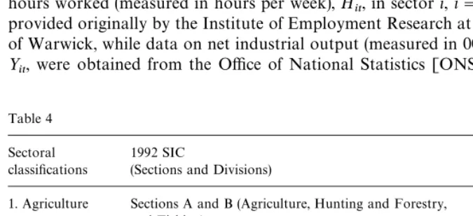
for i"1,2, 8, and where * is the di!erence operator. In what follows we estimate the production relations (5.4) for eight industrial sectors in the UK, using annual data for the period 1954}1995. The industrial classi"cation has been chosen to provide a comprehensive coverage of UK output, and represents the most disaggregated speci"cation for which consistent series for output, employment and capital are available over the whole period.20
While the industrial employment and capital data represent the best measures of the current gross output potential of inputs of labour and "xed assets, respectively, the "gures cannot take into account the extent to which the available factors are actually utilized in production. For the Manufacturing sector, however, survey data is available through the Confederation of British Industries on the proportion of"rms who report that they are operating below full capacity at any time,c
Mt. In this industry, therefore, we are able to adjust the
factor input data to take into account the factor utilisation rate. Speci"cally,
writing the unadjusted capital data in the Manufacturing sector as KIMt, the adjusted capital input is given by
K
Mt"(1!cMt)KI Mt#cMt(1!pMt)KI Mt
"KI
Mt(1!cMtpMt) (5.5)
wherep
Mtrepresents the proportion of capital which is in use averaged across
those"rms who report that they are operating at below full capacity. A similar computation can be employed to obtain an adjusted labour input measure in the Manufacturing sector. While data onKI Mtandc
Mtexists for the Manufacturing
sector, thep
Mtremains unknown. In the empirical work that follows, we assume
that p
Mt is constant over time, and estimate it by the maximum likelihood
method.21
5.1. Productivity dummies
One important advantage of a disaggregate model over an aggregate model is that it is able to incorporate sector-speci"c information which is less easily accommodated within an aggregate model. Particularly relevant to the present application is sector-speci"c shocks to labour productivity that are associated with extreme events such as oil crisis, strikes, and severe weather conditions. For instance, productivity in the agricultural sector is likely to be signi"cantly a!ected by severe weather conditions, even though one might not expect to"nd any signi"cant weather e!ects on labour productivity at the aggregate level in an industrialized economy such as UK.
The e!ects of eight separate events which might have in#uenced labour productivity in the di!erent sectors are incorporated in the empirical analysis through the inclusion of dummy variables in the estimated industrial equations. These are:
dE1
t"1 if t"1972 and 0 otherwise,
dE2
t"1 if t"1974 and 0 otherwise,
dE3
t"1 if t"1984 and 0 otherwise;
dW1
t"1 ift"1975 and 0 otherwise,
dW2
t"1 ift"1976 and 0 otherwise,
dW3
t"1 ift"1984 and 0 otherwise,
21If data were available, a similar adjustment could also be made to factor inputs in other sectors. In the absence of such data, however, the published data are used in their unadjusted form in the other industrial sectors (which is equivalent to assuming that bothc
MtandpMtare constant over
and
dO1
t"1 for t*1974 and 0 otherwise,
dO2
t"1 for t*1980 and 0 otherwise.
(5.6)
The inclusion of the dummiesdE1
t,dE2tanddE3trelates to the strikes experienced in
the Mining and Energy sectors in the UK during the years 1972, 1974 and 1984, respectively. The miners'strike of January}February 1972 resulted in the gov-ernment declaring a state of emergency, power cuts and fuel rationing, and most of British industry went on a 3-day working week. Similarly, industrial action by the miners and by power engineers in the"nal months of 1973 resulted in the government again declaring a state of emergency, the imposition of prohibitions on space heating in industrial and commercial premises and the imposition of a reduced working week during January and February 1974. And the miners'
strike called in the Summer of 1984 resulted in more than 33% of working days being lost in the industry during that year and threats to power supplies across a wide spectrum of British industry. Given the nature of these disputes, it is possible that productivity in any sector would be adversely a!ected in these years, and so the e!ects of these dummies were considered in all eight of our industries.
The dummiesdW1
t,dW2tand dW3t relate to the e!ects of weather conditions on
outputs, and are considered only in the Agriculture sector. The "rst two dummies are intended to capture the e!ects of the severe drought conditions experienced in 1975 and 1976 which considerably reduced Agricultural output during those two years. The third dummy is intended to capture the e!ects of the especially favourable weather conditions experienced during 1984 which resulted in high crop yields and record levels of output for many crops in that year.22
The dummiesdE
jt anddWjt, j"1, 2, 3, aim to capture the e!ects of particular
events which a!ected productivity only temporarily (i.e. in subsequent years, productivity is assumed to return to the level it would have achieved in the absence of the event). In contrast, the dummiesdO1
tanddO2taim to capture the
e!ects of the oil price rises which took place at the end of 1973 and during 1980. It has been argued that these events permanently lowered the level of productiv-ity in many industries, and these dummies take a di!erent form to those relating to the energy sector disputes and weather conditions to re#ect this permanent e!ect. Again, in view of the signi"cance of oil throughout the economy, we considered the e!ect of these shocks in all eight of the industrial sectors.
5.2. Industrial and aggregate production functions
Tables 1a, 1b, 2a and 2b provide the results of estimating equations of the form given in (5.4) for our eight industrial classi"cations. Tables 1a and 1b provides the estimated equations in the absence of any productivity dummies, while Tables 2a and 2b contain the outcome of a speci"cation search in which the productivity dummies are included. Concentrating on Table 1"rst, we"nd that, even without the use of productivity dummies, the log-linear speci"cation given in (5.4) generally provides a reasonable representation of output develop-ments in the eight industries.23 The estimated value ofa
ilies within the [0, 1]
interval in every case, and the variation in the estimated ai's observed across industries appears reasonable on a priori economic grounds.24 The statistics for testing the restrictions of constant returns, which is imposed throughout, are given in Table 1b under the column headed RR
i; these demonstrate that
the restriction is rejected at the 5% level in just two industries (namely, Agriculture and Energy). Since our analysis of log-linear aggregation requires that the same functional form is speci"ed across all the eight industries, despite the rejection of the constant returns restriction in the two of the industries we decided to impose the restriction across all the industries, so that (5.4) can be rewritten to explain the (logarithm of the) output}capital ratio in terms of the (logarithm of the) labour}capital ratio. ReportedR2's show the proportion of the variation in the growth in the output}capital ratio around its mean that is explained by the model; these average approximately 26% over the eight sectors, which is reasonably high given the simplicity of the model. The model has signi"cant explanatory power in all cases except the Energy sector, in which the output growth is dominated exclusively by capital growth. The remaining diagnostic test statistics reported in Table 1b are by and large acceptable, although the normality of residuals is clearly rejected in the Mining and Energy industries. Inspection of the residuals in these industries show some very large outliers,
23The adjustment made to take into account the extent to which factor inputs are utilized in the Manufacturing sector turned out to be qualitatively important. Without making the adjustment (equivalent to settingC
Mt"0 in (5.5)), the estimated equation in the Manufacturing sector is
y
Mt"0.0441#1.1193lMt!0.1193kMt#e(Mt
(5.38) (6.73) (N/A)
with the maximized log-likelihood value of 86.69. Using a grid search the maximum likelihood estimate ofp
Mturned out to be 0.81. This estimate was used in the equations reported in Tables
1a,1b,2a and 2b (with associated maximized log likelihood values of 98.28 and 100.56, respectively).
especially for the years 1972, 1974, and 1984. Of course, these are precisely those years in which prolonged and national strikes took place in the Mining and Energy sectors. Overall, therefore, the results reported in Tables 1a and 1b show that the simple Cobb}Douglas speci"cation, expressed in di!erences, provides a very reasonable representation of output movements in the industries of the UK over the sample period, and the disaggregate model will be further im-proved if the obvious productivity shocks that were experienced in some industries are taken into account through the inclusion of the productivity dummies described in (5.6).
The equations in Table 2a report the outcome of a speci"cation search in which the Cobb}Douglas production function is supplemented with the produc-tivity dummies. The most general speci"cation for all industries other than Agriculture included the dummies relating to energy and oil shocks (i.e. dEjt,
j"1, 2, 3, anddO
jt,j"1, 2); in the Agriculture sector, these"ve dummies were
supplemented with the productivity dummies relating to weather conditions. In
Table 1a
Estimates of industrial production functions (1956}1995)
Sectors k(
i a(i (1!a(i)
Agriculture 0.0266 0.4276 0.5724
(0.001) (0.208) (*)
Mining 0.0185 0.5951 0.4049
(0.031) (0.240) (*)
Manufactures 0.0166 0.4948 0.5052
(0.006) (0.125) (*)
Energy 0.0309 0.1092 0.8908
(0.017) (0.304) (*)
Construction 0.0143 0.7454 0.2546
(0.008) (0.114) (*)
Transport 0.0263 0.5950 0.4050
(0.005) (0.163) (*)
Communications 0.0331 0.6327 0.3673
(0.008) (0.162) (*)
Other Services 0.0056 0.6451 0.3549
(0.010) (0.183) (*)
Average
(Mean group estimate) 0.0215 0.5306 0.4694
Note: Results relate to regression equations of the form
*y
it"ki#ai*lit#(1!ai)*kit#eit,
fori"1, 2,2, 8, and where standard errors are provided in parentheses. The&mean group estimate'
Table 1b
Diagnostic statistics for the estimated production functions in Table 1a
Sectors R2 p(
i ¸¸Fi RRi qi SCi FFi Ni Hi
Agriculture 0.0999 0.0576 58.4266 5.2807 1 1.8571 5.5886 1.7777 1.6680
Mining 0.1390 0.1228 28.1578 1.8637 1 3.8204 0.2232 162.2353 0.1561
Manufactures 0.5435 0.0213 98.2887 0.1719 1 0.4427 0.0876 0.6902 0.4918
Energy 0.0034 0.0600 56.7965 0.1100 1 3.9271 0.1586 45.0702 0.8085
Construction 0.5284 0.0394 73.6196 0.5331 1 2.2092 1.5060 3.9545 0.3440
Transport 0.2598 0.0297 84.9039 2.2021 1 1.6748 3.2959 0.2750 0.0292
Communications 0.2865 0.0276 87.8917 6.5421 1 1.9919 4.9257 2.1829 5.8440
Other Services 0.2463 0.0240 93.4500 1.4193 1 5.0344 2.1355 1.6287 2.8302
Note: Diagnostic statistics relate to the equations presented in Table 1a.R2denotes the proportion of the variation in the growth in the output}capital
ratio around its mean that is explained by the model;p(
iis the estimated standard error of the regression;¸¸Fiis the value of the log-likelihood;RRiis the
test of theq
irestriction(s) imposed on the regression (i.e. the&constant returns to scale'restriction in Table 1a, cf.F(1, 38));SCirefers to Breusch and
Pagan's LM test of"rst-order serial correlation in the residuals (cf.s2(1));FF
irefers to Ramsey's RESET test of the functional form of the regression (cf.
s2(1));N
irefers to Bera and Jarque's test of the normality of the residuals (cf.s2(2)); andHitests the presence of heteroskedasticity in the residuals (cf.s2(1)).
Further details on the form of the tests is provided in Pesaran and Pesaran (1997).
K.J.
v
an
Garderen
et
al.
/
Journal
of
Econometrics
95
(2000)
285
}
Estimates of industrial production functions (including productivity dummies, 1956}1995)
Sectors k(
i a(i (1!a(i) bKE1i bKE2i bKE3i bKW1i bKW2i bKW3i bKO1i bKO2i
Agriculture 0.0275 0.4572 0.5428 * * * !0.0812 !0.1386 0.1241 * *
(0.009) (0.158) (!) (0.036) (0.036) (0.031)
Mining 0.0033 0.4470 0.5530 !0.1257 !0.1126 !0.4758 * * * * *
(0.011) (0.088) (!) (0.032) (0.032) (0.031)
Manufactures 0.0165 0.4929 0.5071 * * !0.0304 * * * * *
(0.006) (0.119) (!) (0.014)
Energy 0.0285 0.0576 0.9424 * * !0.2052 * * * * *
(0.011) (0.190) (!) (0.027)
Construction 0.0171 0.6937 0.3063 * * * * * * !0.1294 !0.0703
(0.007) (0.097) (!) (0.034) (0.033)
Transport 0.0275 0.5682 0.4318 * * * * * * * !0.0601
(0.005) (0.157) (!) (0.029)
Communications 0.0331 0.6327 0.3673 * * * * * * * *
(0.008) (0.162) (!)
Other Services 0.0083 0.6737 0.3263 * * * * * * * !0.0515
(0.010) (0.175) (!) (0.023)
Average
(Mean group 0.0202 0.5029 0.4971 !0.0157 !0.0141 !0.0889 !0.0102 !0.0173 0.0155 !0.0162 !0.0227
estimates)
Note: Results relate to equations of the form
*y
it"ki#ai*lit#(1!ai)*kit#
3 +
j/1
bEji*dEjt#+3
j/1
bWji*dWjt#+2
j/1
bOji*dOjt#e
it,
i"1, 2,2, 8, where the dummy variables,dJjt, are de"ned in (5.6) in the text. Standard errors are provided in parentheses.
K.J.
v
an
Garderen
et
al.
/
Journal
of
Econometrics
95
(2000)
285
}
331
Table 2b
Diagnostic statistics for the estimated industrial production functions in Table 2a Sectors R2i p(
i ¸¸Fi RRi qi SCi FFi Ni Hi
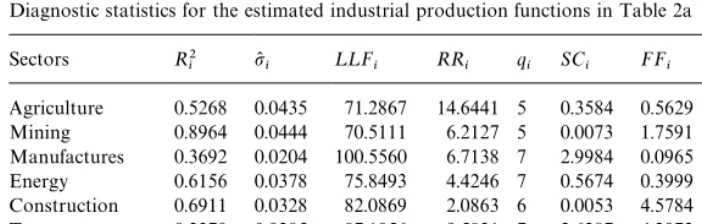
Agriculture 0.5268 0.0435 71.2867 14.6441 5 0.3584 0.5629 1.6335 0.3588 Mining 0.8964 0.0444 70.5111 6.2127 5 0.0073 1.7591 56.4326 0.0230 Manufactures 0.3692 0.0204 100.5560 6.7138 7 2.9984 0.0965 0.5495 0.7003 Energy 0.6156 0.0378 75.8493 4.4246 7 0.5674 0.3999 3.0886 0.3557 Construction 0.6911 0.0328 82.0869 2.0863 6 0.0053 4.5784 0.6423 0.0612 Transport 0.3370 0.0285 87.1056 9.5831 7 2.6287 4.2973 0.2077 0.1357 Communications 0.2865 0.0276 87.8917 14.2207 8 1.9919 4.9257 2.1829 5.8440 Other Services 0.3349 0.0229 95.9498 9.3691 7 6.3481 2.1926 1.8472 3.1937 Note: Diagnostic statistics relate to the equations presented in Table 2a. See also notes to Table 1b.
the regression results reported in Table 2a, dummies were excluded if they failed to be statistically signi"cant at the 5% level.25Once again, the regression results are encouraging. The reported R2's now lie in the range (0.33, 0.90), and the average value across the eight sectors is 51%. The diagnostic statistics provided in Table 2b indicate that there are few problems with residual serial correlation, functional form, the normality of residuals or heteroskedasticity. The weather dummies take coe$cients of a sensible order of magnitude in the Agriculture equation and, as expected, the e!ects of the mining and energy sector strikes all showed signi"cantly in the Mining industry. However, only the e!ect of the 1984 dispute has a signi"cant e!ect outside the Mining industry, and then only in the Manufacturing and Energy sectors. There is evidence of a fall in productivity, as captured by the dummiesdO1
tanddO2t, in three of the industrial sectors (namely,
Construction, Transport and Other Services). The fact that these e!ects are observed in these particular industries casts some doubt on the interpretation of their e!ects, however; the dummies are intended to capture the e!ects of oil price shocks, but these industries are not those which one would have expected to be particularly a!ected by oil prices a priori. On the other hand, in the estimated regressions, these dummies take the form of a simple intercept correction in the speci"ed period, and e!ectively capture the e!ects of unusually large productiv-ity shocks experienced in these industries in 1974 and 1980. In what follows, therefore, we continue to include the e!ects of the oil price dummies in these industries, while recognizing the di$culty that surrounds their interpretation.
25A joint test of the insigni"cance of the excluded variables shows that the speci"cation search is acceptable in every case. In Table 2b, the statisticRR
iprovides the test statistic relating to all the