High-resolution modeling of LIDAR data
Mechanisms governing surface water
vapor variability during SALSA
C.-Y.J. Kao
∗, Y.-H. Hang
1, D.I. Cooper, W.E. Eichinger
2, W.S. Smith, J.M. Reisner
Los Alamos National Laboratory, Los Alamos, NM 87545, USA
Abstract
An integrated tool that consists of a volume scanning high-resolution Raman water vapor LIDAR and a turbulence-resolving hydrodynamic model, called HIGRAD, is used to support the semi-arid land-surface–atmosphere (SALSA) program. The water vapor measurements collected during SALSA have been simulated by the HIGRAD code with a resolution comparable with that of the LIDAR data. The LIDAR provides the required “ground truth” of coherent water vapor eddies and the model allows for interpretation of the underlying physics of such measurements and characterizes the relationships between surface conditions, boundary layer dynamics, and measured quantities. The model results compare well with the measurements, including the overall structure and evolution of water vapor plumes, the contrast of plume variabilities over the cottonwoods and the grass land, and the mid-day suppression of turbulent activities over the canopy. The current study demonstrates an example that such an integration between modeling and LIDAR measurements can advance our understanding of the structure of fine-scale turbulent motions that govern evaporative exchange above a heterogeneous surface. © 2000 Elsevier Science B.V. All rights reserved.
Keywords: Water vapor LIDAR data; Canopy effects; Hydrodynamic model; Small-scale eddies; Water vapor variability
1. Introduction
During the semi-arid land-surface–atmosphere (SALSA) program led by USDA-ARS in August 1997 over southeastern Arizona (Goodrich et al., 2000), Los Alamos National Laboratory (LANL) fielded an advanced scanning Raman LIDAR as part of the larger suite of meteorological sensors. The LANL LIDAR was utilized to quantify processes associated with the evapotranspiration (ET) over a cottonwood riparian corridor and the adjacent mesquite-grass
∗Corresponding author.
1On leave from Institute of Applied Physics and Computational Mathematics, Beijing, China.
2University of Iowa, Iowa City, IA 52242, USA.
region, and furthermore, their interaction with the atmospheric boundary layer. The LANL volume scanning Raman LIDAR has been demonstrated in numerous field experiments to produce water vapor concentration patterns with spatial resolution of 1.5 m (e.g., Eichinger et al., 1993, 1994; Cooper et al., 1994, 1996, 1997). LIDAR data of this kind have been processed by statistical methods and validated with conventional tower-mounted eddy flux systems in the above studies. On the other hand, these data sets have also shown us that the time–space structure measured by the LIDAR can yield interpretations that go be-yond what conventional analyses can offer (Cooper et al., 1997). This required us to utilize an ultra-high resolution hydrodynamic model to investigate the possible underlying physics for the temporal and
spatial evolution of water vapor revealed by LIDAR. To this end, a relatively new hydrodynamic model (Reisner and Smolarkiewicz, 1994; Smolarkiewicz and Margolin, 1993; Kao et al., 2000) for simulating high-gradient flows such as those that LIDAR can re-solve has been utilized for integration purposes with our LIDAR-measured water vapor data at a resolution of meters.
The ultimate goal of this project is to use very high temporal and spatial resolution water vapor obser-vations and an ultra-high resolution eddy simulation atmospheric model to observe and understand the transport mechanisms of humidity in the atmospheric surface and boundary layers. The resulting level of physical understanding should guide significant im-provements in the parameterization of latent heat eddy fluxes over land surfaces with proper and con-sistent dependencies on stability and meteorological quantities.
A reliable parameterization of land-surface–atmos-phere exchanges of heat, moisture, and momentum requires a fully quantitative understanding of the near-surface distribution of these scalars and their evolution. One of the basic problems in studying the moisture exchange in the surface–atmosphere interac-tion is the determinainterac-tion of the minimum scale neces-sary to describe the water vapor variability (Lawford, 1996). In other words, what is the water vapor distri-bution at the scale of coherent eddies (or the water va-por plumes)? The satellite-based data sets upon which present global environmental assessments depend un-fortunately cannot answer this question and neither can any conventional point measurement platforms. In this paper, we demonstrate that a unique combination of two complementary capabilities, respectively, for measurement and modeling, can help to address is-sues of variability of near-surface and boundary-layer water vapor and associated transport mechanisms.
In the current modeling study, we first simulate the general aspects of formation and evolution of coher-ent plumes idcoher-entified by the LIDAR over the SALSA surface within a convectively unstable boundary layer from the mid-morning to the early afternoon. The contrast of plume variability over the cottonwood canopy and grassland is also investigated based upon the model design assumption that the canopy is treated as a moisture source and a momentum sink. We are particularly interested in an event observed by the
LIDAR, that indicates that the microscale plumes ap-pear to weaken during mid-day over cottonwoods. It is a phenomenon which is not supported by conven-tional wisdom of the convective boundary layer.
Section 2 of this paper presents a brief review of the water vapor Raman LIDAR and the data collected dur-ing SALSA. Section 3 introduces the hydrodynamic model and related model physics. Section 4 shows the simulation design. Section 5 presents model results and their comparison with observations. Finally, Sec-tion 6 provides a summary and concluding remarks.
2. LIDAR data on 11 August 1997
For more than two decades, LIDAR (LIght Detec-tion And Ranging) remote sensing technology has of-fered the promise of prompt, nearly instantaneous, and multi-dimensional atmospheric measurements to ranges of 1–10 km with spatial resolution of a few me-ters, providing the degree of detail necessary to de-scribe boundary layer phenomena. The LIDAR used in SALSA is a self-contained field deployable UV Raman water vapor system (Eichinger et al., 1992, 1994). It uses an excimer laser source with 400 mJ per pulse of energy at 200 Hz at wavelengths of 248 and 351 nm. The receiver uses a 24 in. f8 telescope and scanning optics to allow 3D volumetric imaging of water vapor mixing ratio and extraction of 2D surface fluxes.
the two regions in terms of the absolute values as well as the temporal and spatial variability is quite large.
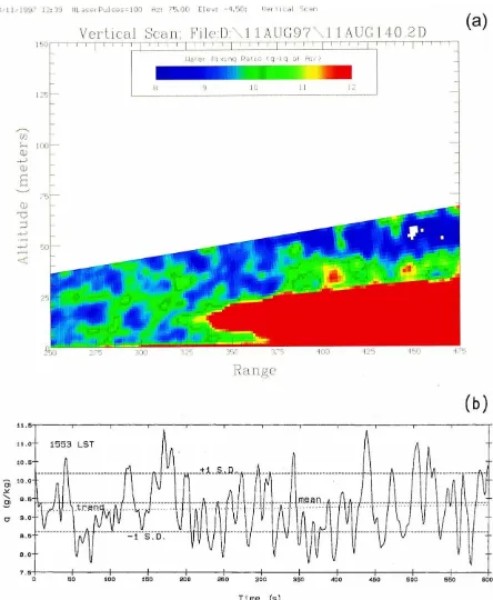
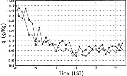
Fig. 1a shows one snapshot of the water vapor mix-ing ratio in a vertical slice measured by the Raman system over the canopy, represented by the bottom red region in the figure, at 1436 LST on 11 August 1997. Note that Fig. 1a simply overlaps the frame number 5 in Fig. 3 of Cooper et al. by 100 m in the horizon-tal range. The image shows 10–20 m diameter moist plumes surrounded with high spatial gradient between 500 and 575 m in range. Fig. 1b, on the other hand, shows the time series of LIDAR-measured water va-por concentrations at 10 m above the canopy starting from 1553 LST. Fig. 1a and b together demonstrates the LIDAR capability in capturing the high-resolution variability of water vapor near the top of the canopy.
D.I. Cooper (1998, private communication) was not certain that the plumes in Fig. 1a were real signals due to the range concerns (as uncertainty is proportional to range), and did not include them, therefore, in their observation paper. We believe, however, that there is a dynamic support for these plumes, as will be discussed in Section 5. Fig. 1a also shows fine structure of dry eddies between 375 and 475 m in range, penetrating downward presumably from the mixed layer. Such an interaction between the surface layer and mixed layer within a convective boundary layer has been docu-mented both over land (e.g., Williams and Hacker, 1993) and oceans (e.g., Cooper et al., 1997).
3. Model
As LIDAR technology is able to provide data at a resolution of meters in a 3D atmospheric volume, it is imperative to promote a modeling counterpart of such a LIDAR capability. The hydrodynamic model used for the current work is an outgrowth of the numerical modeling framework of Reisner and Smolarkiewicz (1994) and Smolarkiewicz and Margolin (1993). It is a nonhydrostatic model with the option of being anelas-tic (Smolarkiewicz and Margolin, 1994) or fully com-pressible (Reisner and Kao, 1997).
The model is based on a nonoscillatory forward-in-time advection scheme (MPDATA, see Smolarkiewicz and Margolin, 1998). It has the advantage of preser-ving both local extrema and the sign of the transported properties. The scheme assures solutions consistent
with analytic properties of the modeled system and minimizes the need for artificial viscosity, while sup-pressing nonlinear computational instabilities. The pressure equation is solved with an efficient conju-gate gradient scheme (Smolarkiewicz and Margolin, 1994), which is flexible and efficient without re-quiring any knowledge of the discretized elliptical operators’ coefficient matrix. Overall, the model is designed to be used to accurately model small-scale atmospheric dynamics with high-gradient features; hence it is referred to as HIGRAD.
Other numerical options include a sound-wave temporal averaging scheme (Reisner and Kao, 1997) to effectively filter the sound waves; and the “volume of fluid” (VOF) method (Kao et al., 2000) which can track the boundaries of materials such as clouds and tracer species. The radiation parameterization is adapted from Smith and Kao (1996). Surface temper-ature is parameterized using a five-layer subsurface model with parameterized surface fluxes of heat and moisture, specified albedo and emissivity for the surface, and specified heat capacity and thermal con-ductivity for each layer. The surface fluxes of heat and moisture are calculated with a surface parameter-ization based on Monin–Obuhkov similarity theory.
4. Simulation design
In order to match the actual dimensions of the do-main over which LIDAR measurements were reported in Cooper et al. (2000), we configure a 2D model domain of 500 m (horizontal) ×1000 m (vertical).
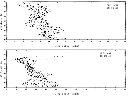
Fig. 2. Vertical profiles of LIDAR-measured water vapor over the canopy between 425 and 450 m in the horizontal range for 0913 and 1156 LST.
upper boundary. Cyclic boundary conditions are used at lateral boundaries. We prescribe all the subgrid transports with a small diffusivity coefficient (km) at a constant value of 10−6m2s−1. Our model tion is somewhat similar to direct numerical simula-tions (DNSs) at least in terms of small1z and small kmnear the surface.
With the very high model resolution described above, the cottonwood canopy at the SALSA site can almost be resolved, but not quite. This makes exist-ing parameterizations of canopy effects not entirely applicable to our model. On the other hand, our res-olution is still too coarse to model each individual cottonwood tree. A novel way to reach a compromise in resolution is required. We adopt the approach by Kaimal and Finnigan (1994) to identify the so-called
displacement height within the canopy, which is about 70% of the average tree height. Below the displace-ment height, the modisplace-mentum becomes zero and the thermodynamic variables become constant with alti-tude. We choose a value of 10 m for the displacement height in the model, which implies that the average tree height is about 15 m. This model design approxi-mates the canopy as an impermeable rectangular block with a dimension of 10 m high and 150 m wide with time-constant thermodynamic properties (cf. Fig. 4).
sea level). These conditions made the simulation more tractable since the effects due to large-scale variation with time were not a major concern.
The model simulations were initialized at 0600 LST, an hour before the transition period of the bound-ary layer started. Based on the tower and rawindsonde data, the initial potential temperature was assumed to be a constant of 303.0 K from the surface to 500 m above the surface. A moist adiabatic lapse rate of tem-perature was assumed for the rest of the model depth. The initial water vapor from the surface to 500 m was 11.5 g kg−1. A lapse rate of 7.0 g kg−1km−1was assumed for the rest of the model depth. At the top of, and within the canopy, the water vapor concentra-tion was initialized at 20.5 g kg−1; this value will be discussed further below. To excite an initial distur-bance, a random distribution of temperature with a standard deviation of 0.01 K was imposed at the surface. The initial momentum field was set to be westerly at a wind speed of 2 ms−1.
5. Results of model simulation
In order to approximate the water vapor forcing due to canopy to the atmosphere without incorporating a biological component in the modeled system, we use the LIDAR data to estimate the time change of wa-ter vapor mixing ratio at the top of the canopy. Fig. 2 shows the water vapor profiles measured by LIDAR over the canopy between 30 and 70 m above the sur-face at 0913 and 1156 LST. The averaged difference between the two profiles is about 2 g kg−1. The dif-ference right above the canopy is about 5 g kg−1, rep-resenting a rate of water vapor decrease as significant as 5 g kg−1in 3 h. This rate is prescribed at the top of the modeled canopy. We did not have any extra treat-ment for the temporal water vapor variation over the grass as we did over the canopy, since the grass is not considered as a major source for the coherent eddies observed. Instead, we just let the model evolve with time over the grass with the initial conditions stated in Section 4.
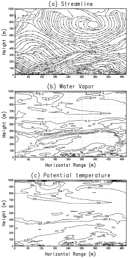
With a neutral initial condition for potential tem-perature at 0600 LST (see Section 4), it takes the model about 2 h to develop a near-surface unstable layer driven by the radiative shortwave absorption at the surface. In the mean time, a well-defined
bound-ary layer circulation pattern and associated thermody-namic properties begin to develop as seen in Fig. 3, where circulation streamlines (Fig. 3a), water vapor (Fig. 3b), and potential temperature (Fig. 3c) are shown for 0800 LST of the simulation. All of the above fields indicate a mixed-layer height of about 400 m with a rather weak capping inversion in terms
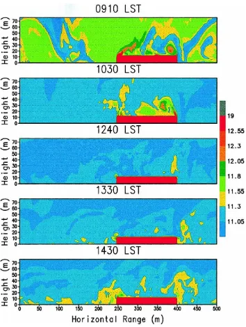
Fig. 4. Simulated water vapor field (g kg−1) with a contour interval of 0.5 from 0910 to 1430 LST in comparison with Fig. 3 of Cooper et al. (2000). Note that the horizontal range in the current figure is from west to east.
of the changes of potential temperature and water va-por with height. The maximum wind speed is about 5 ms−1and is near the top of the mixed layer.
As the solar heating at the surface increases with time, the inversion becomes even less distinct and
eventually the entire vertical domain (1 km) becomes well mixed.
layer as apparent in both the water vapor (Fig. 3b) and potential temperature (Fig. 3c) fields. In Fig. 3a, the small near-surface eddies less than 100 m in vertical extent in the vicinity of the canopy (from 250 to 400 m along the horizontal axis, cf. Fig. 4) are caused by the momentum sink due to the canopy as discussed in the previous section. These eddies correspond to the near-surface plumes in water vapor and potential temperature shown in Fig. 3b and c.
Fig. 4 shows the modeled water vapor field as a counterpart of the measured field, shown in Fig. 3 (Cooper et al., 2000), and Fig. 1a. The spatial structure of the simulated water vapor plumes and their time evolution are in good agreement with the observations. The agreement includes the following: (i) the upward-tilting “ramps” of higher water vapor content over the canopy identified in the LIDAR im-ages are captured by the model simulation; (ii) the variability of water vapor content over the canopy is higher than that over the grassland; and (iii) no plumes are either observed or modeled over the grassland in the afternoon. Interestingly, the model results also indicate that the convective plumes over the canopy are more active in the morning hours than in the early afternoon hours, despite the fact that the convec-tion should be more rigorous in the early afternoon. More discussion and explanation about this mid-day turbulence suppression will be given later.
Fig. 5 represents the counterpart of Fig. 5a in Cooper et al. (2000), showing the vertically averaged water vapor as a function of time over the canopy and grassland. The two figures are in good agreement in that higher water vapor values and larger temporal variability are seen for the region over the canopy. The range of variation for water vapor is, however, considerably smaller in the modeled case. This is probably due to the differences in data sampling. Note that Cooper et al. (2000) used a 25 m scan width for constructing Fig. 5a, while the entire physical areas of the canopy and the grassland specified in the model are used in constructing Fig. 5 in this paper.
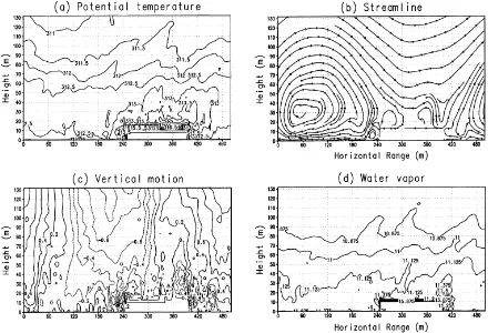
To explain the suppressed plume activity over the canopy in the early afternoon (Fig. 4), we first show the potential temperature averaged from 1230 to 1430 LST (Fig. 6a). The potential temperature over the canopy is higher than that over the grassland; this agrees with the observations made by airborne thermal remote sensing of skin temperature over the
Fig. 5. Simulated vertically averaged water vapor over the cotton-wood canopy (solid circles) and the grassland (open circles) from 0900 to 1430 LST.
Bosque del Apache Research Site in southern New Mexico (C. Neale, 1999, private communication). The potential temperature over the canopy within this period is basically characterized by an unstable strat-ification, which, in principle, should be favorable for plume activity. However, the prevailing westerlies up to 10 ms−1associated with Fig. 6b complicate the sit-uation. Together with the higher potential temperature over the canopy, they generate the downward motion above the canopy’s western part (Fig. 6c) and the sur-face outflows right at the top of the canopy (Fig. 6b). The downward motion suppresses plume growth over the central part of the canopy, and the upward motion over the eastern part of the canopy promotes some limited plume activity, as seen in panels (c) and (d) of Fig. 4. To summarize, we observe the disloca-tion of upward modisloca-tion by mean winds over a low-level heated air mass. As a result, the downward motion occupies most of the heated canopy. The standing cir-culation west of the canopy is the result of this dis-location plus the cyclic lateral boundary conditions used in the model. In other words, if the prevailing westerlies were not present, we would have observed the upward motion right above the heated canopy and the downward motion on the two sides. Reisner and Smolarkiewicz (1994) presented a thorough review of flows past heated obstacles. The case presented here is consistent with their analysis.
Fig. 6. Simulated: (a) potential temperature with a contour interval of 0.5 K; (b) streamline; (c) vertical motion with a contour interval of 0.2 ms−1; (d) water vapor with a contour interval of 0.125 g kg−1. All are averaged from 1200 to 1430 LST.
seen in Fig. 6c, at the edges of the canopy. These near-edge upward motions are responsible for the near-edge plumes in the afternoon seen in Figs. 4 and 6d. The above discussion also implies that the plumes seen in Fig. 1a can be real LIDAR signals due to the canopy’s downstream “edge” effects.
6. Concluding remarks
In this paper, we have demonstrated an integrated tool that comprises high-resolution LIDAR mea-surements and advanced modeling capabilities for a fundamental understanding of microscale convective structure including plumes and the turbulent eddies of water vapor over a cottonwood riparian zone. The role of our HIGRAD model simulations in the imple-mentation of a LIDAR measurement strategy enters at
The HIGRAD model is not only able to simulate the general structure and evolution of the observed water vapor plumes during SALSA (Cooper et al., 2000), but also offers a possible explanation of the mechanism for the mid-day suppression of turbulent activity over the cottonwood canopy. The suppression appears to be the result of the higher temperature over canopy than that over the grassland as well as the prevailing wester-lies. They together induce downward motion into the surface layer at the top of the canopy. Unfortunately, we do not have simultaneous measurements of tem-perature over both the canopy and the grassland during SALSA to verify our finding. This research, however, justifies the current development of the next genera-tion of the LANL Raman system that is capable of measuring both water vapor content and temperature.
Acknowledgements
We would like to thank Dr. David Goodrich for his data support and Drs. Peter Smolarkiewicz and Len Margolin for their model support. Thanks are due to Dr. Howard Hanson for stimulating discussions and suggestions concerning the manuscript. The devel-opment of the collaboration between the Institute of Applied Physics and Computational Mathematics in China and Los Alamos National Laboratory was con-ducted by Drs. Willie Hsue and John Shanon under the auspices of the US Department of Energy (DOE). The Institute of Geophysics and Planetary Physics (IGPP) at LANL provided the computing support. This re-search was supported by the US DOE. Support from the NSF-STC SAHRA (Sustainability of Semi-Arid Hydrology and Riparian Areas) under Agreement No. EAR-9876800 is gratefully acknowledged.
References
Cooper, D.I., Eichinger, W.E., Hof, D., Jones, D., Quick, C.R., Tiee, J.J., 1994. Observations of coherent structures from a scanning LIDAR. Agric. For. Meteorol. 67, 137–150. Cooper, D.I., Eichinger, W.E., Barr, S., Cottingame, W.,
Hynes, M.V., Keller, C.F., Lebeda, C.F., Poling, D.A., 1996. High resolution properties of the equatorial Pacific marine atmospheric boundary layer from LIDAR and radiosonde observations. J. Atmos. Sci. 53, 2054–2075.
Cooper, D.I., Eichinger, W., Ecke, R., Kao, C.-Y.J., Reisner, J.M., 1997. Initial investigations of micro-scale cellular convection
in an equatorial marine atmospheric boundary layer revealed by LIDAR. Geophys. Res. Lett. 1, 45–48.
Cooper, D.I., Eichinger, W.E., Hipps, L., Kao, C.-Y.J., Reisner, J., Smith, S., Schaeffer, S.M., Williams, D.G., 2000. Spatial and temporal properties of water vapor and flux over a riparian canopy. Agric. For. Meteorol. 105, 161–183.
Eichinger, W.E., Cooper, D.I., Holtkamp, D., Karl, R.R., Moses, J., Quick, C.R., Tiee, J.J., 1992. Derivation of water vapor fluxes from LIDAR measurements. Boundary Layer Meteorol. 63, 39–64.
Eichinger, W.E., Cooper, D.I., Parlange, M., Katul, G., 1993. The application of a scanning water Raman-LIDAR as a probe of the atmospheric boundary layer. IEEE Geosci. Remote Sensing 31, 70–79.
Eichinger, W.E., Cooper, D.I., Archuleta, F.L., Hof, D., Holtkamp, D.B., Karl, R.R., Quick, C.R., Tiee, J.J., 1994. Development of a scanning solar blind water Raman-LIDAR. Appl. Opt. 33, 3923–3932.
Goodrich, D.C., Scott, R., Qi, J., Goff, B., Unkrich, C.L., Moran, M.S., Williams, D., Schaeffer, S., Snyder, K., MacNish, R., Maddock, T., Pool, O., Chehbouni, A., Cooper, D.I., Eichinger, W.E., Shuttleworth, W.J., Kerr, Y., Marsett, R., Ni, W., 2000. Seasonal estimates of riparion evapotranspiration using remote and in situ measurements. Agric. For. Meteorol. 105, 285–312.
Kaimal, J.C., Finnigan, J.J., 1994. Atmospheric Boundary-layer Flows: Their Structure and Measurement. Oxford University Press, Oxford, 289 pp.
Kao, C.-Y.J., Hang, Y.H., Reisner, J.M., Smith, W.S., 2000. Test of volume-of-fluid (VOF) method over marine boundary layer clouds. Mon. Weath. Rev. 128, 1960–1970.
Lawford, R., 1996. Some scientific questions and issues for the GEWEX Continental-scale International Project (GCIP) research community. In: Proceedings of the Second International Science Conference on Global Energy and Water Cycle, June 17–21, Washington, DC, pp. 162–167.
Reisner, J.M., Kao, C.-Y.J., 1997. Explicit numerical techniques for increasing the efficiency of a forward-in-time shallow water code on a sphere. Parallel Computational Fluid Dynamics. Elsevier, Amsterdam, pp. 453–460.
Reisner, J., Smolarkiewicz, P.K., 1994. Effects of surface thermal forcing on flow past isolated obstacles. J. Atmos. Sci. 51, 117– 133.
Smith, W.S., Kao, C.-Y.J., 1996. Numerical simulations of stratiform clouds observed in 1987 FIRE IOP with the emphasis on diurnal variation. Data Mon. Weath. Rev. 8, 1803–1816. Smolarkiewicz, P.K., Margolin, L.G., 1993. On forward-in-time
differencing for fluids: extension to a curvilinear framework. Mon. Weath. Rev. 121, 1847–1859.
Smolarkiewicz, P.K., Margolin, L.G., 1994. Variational solver for elliptic problems in atmospheric flows. Appl. Math. Comput. Sci. 4, 527–551.
Smolarkiewicz, P.K., Margolin, L.G., 1998. MPDATA: a finite-difference solver for geophysical flows. J. Comput. Phys. 140, 459–480.