A simple water and energy balance model designed for
regionalization and remote sensing data utilization
G. Boulet
a,b,∗, A. Chehbouni
b, I. Braud
a, M. Vauclin
a, R. Haverkamp
a, C. Zammit
aaLTHE CNRS UMR 5564 UJF INPG IRD, BP 53, 38041 Grenoble Cedex 9, France bIRD/IMADES, Reyes y Aguascalientes, 83190 Hermosillo, Sonora, Mexico
Abstract
A simple soil–vegetation–atmosphere transfer (SVAT) model designed for scaling applications and remote sensing utiliza-tion will be presented. The study is part of the Semi-Arid Land Surface Atmosphere (SALSA) program. The model is built with a single-bucket and single-source representation with a bulk surface of mixed vegetation and soil cover and a single soil reservoir. Classical atmospheric forcing is imposed at a reference level. It uses the concept of infiltration and evaporation capacities to describe water infiltration or exfiltration from a bucket of depth drcorresponding to the average infiltration and
evaporation depth. The atmospheric forcing is divided into storm and interstorm periods, and both evaporation and infiltration phenomena are described with the well-known three stages representation: one at potential (energy- or rainfall-limited) rate, one at a rate set by the soil water content and one at a zero rate if the water content reaches one of its range limits, namely saturation or residual values. The analytical simplicity of the model is suitable for the investigation of the spatial variability of the mass and energy water balance, and its one-layer representation allows for the direct use of remote sensing data. The model is satisfactorily evaluated using data acquired in the framework of SALSA and a mechanistic complex SVAT model, Simple Soil-Plant-Atmosphere Transfer (SiSPAT) model. © 2000 Elsevier Science B.V. All rights reserved.
Keywords: SVAT modeling; Remote sensing; Infiltration and exfiltration capacities
1. Introduction
Detailed soil–vegetation–atmosphere transfer (SVAT) models, especially when they exhibit small time and space steps, are difficult to use for the investigation of the spatial and temporal variability of land surface fluxes. The large number of parameters they involve (physical or geometrical parameters as well as parameters appearing in the empirical relationships) requires detailed field studies and experimentation to derive parameter estimates. Moreover, classical experimental set-ups give local values, whereas larger-scale (i.e. grid) values would be required. On the other hand, running these models for each point location is intractable (Boulet et al., 1999a). Inversion procedures using remote-sensing data can provide some of these parameters (Soer, 1980; Brunet et al., 1994; Camillo, 1991; Kreiss and Rafy, 1993; Taconet et al., 1995; Olioso et al., 1995). But their mathematical implementation will be more robust if the number of unknown parameters is restricted (Duan et al., 1992; Franks et al., 1997; Gupta et al.,
∗Corresponding author. Present address: CESBIO, 18 av. E. Belin, bpi 2801, 31401 Toulouse Cedex 4, France. Tel.:+33-5-61-55-66-70; fax:
+33-5-61-55-85-00.
E-mail address: [email protected] (G. Boulet).
1998). In order to fulfill this requirement for large-scale applications and relatively long time-series, very simple water-balance models have been developed. They are usually based on a simple-bucket representation (Eagleson, 1978a–f; and especially Eagleson, 1978c). Three possible ways of calculating the ‘bulk’ evaporation are described in the literature:
1. The electrical analogy is applied with a surface resistance rs, depending on the bucket water contentθ (soil, vegetation or bulk surface resistance to water vapor extraction) in series arrangement with the aerodynamic resistance ra:
Le=ρcp γ
esat(Ts)−ea ra+rs
(1)
where Le is the latent heat flux, L the latent heat of vaporization, e the evaporation rate,ρthe air density, cpthe specific heat of air,γ the psychrometric constant, esat(Ts) the saturated vapor pressure at temperature Ts, Tsthe surface temperature and where eais the air vapor pressure at reference level.
2. A proportionality relationship is assumed with the potential evaporation rate epthrough a soil moistureθ-dependent function called ‘β-function’:e=βepor Le=βLep.
In a SVAT model inspired by Eagleson (1978c), Kim et al. (1996) propose an analytical scheme combining a physical description of infiltration together with aβ-function approach whereβis simply the ratio between the actual and the saturated bucket water content:
β= θ
θsat (2)
According to Kim et al. (1996), this method leads to a realistic description of cumulated and instantaneous total evaporation E and e over long periods of time but tends to underestimate the instantaneous evaporation rate e at the beginning of each drying period and overestimate e at the end of each drying period.
3. An analytical approximation of the mechanistic transfer equations (desorptive approach) is used to retrieve the soil effect on the surface water availability.
Evaporation is equal to the minimum value of both potential evaporation and an evaporation capacity given by
e≈ Sd 2√t −
K0
2 (3)
where Sdis the desorptivity, t the time (with origin at the beginning of the interstorm) and where K0is the initial hydraulic conductivity value at initial water contentθ0.
Kim et al. (1996) take the percolation into account together with the above-mentioned ‘β-function’ and derive E analytically. This leads to an exponential decay of e:
e≈A(ep, θ0,soil)exp
− ept drθsat
(4)
where A depends onθ0, ep, the soil hydraulic properties and dr, the hydrologically active depth. The characteristic time of this exponential decay is
τ = drθsatln(2)
ep (5)
Although the desorptive approach has been initially proposed for bare soils, it has been extended by Eagleson (1978c) to all natural surfaces, and incorporated in the GCM surface schemes of Entekhabi and Eagleson (1989) and Famiglietti and Wood (1992). The validity of this approach has been widely checked (in natural environment and laboratory columns) for bare soil, but few articles have been published showing its validity for natural grasslands (Brutsaert and Chen, 1995; Salvucci, 1997). These authors have stated that, especially if the rooting zone is not too deep and if the vegetation is likely to be stressed or close to stressed conditions (i.e. if the transition phase, where roots takes water from the lower levels of the soil, is reduced to a minimum), this simple approach can be successfully applied to a sparse short vegetation cover in a relatively arid environment. When vegetation is present, the physical identification of the remotely sensed inversed/retrieved soil hydraulic parameters is difficult to infer, since they account for both soil and root/plant transport. They should be seen as bulk parameters, and the investigation might be restricted to the local evaluation of the main resulting parameters. In the case of taller (shrubs, trees) or more developed (dense crops) vegetation, the model could be adapted in a force-restore scheme by adding a deeper layer corresponding to the rooting zone.
We will present in this paper a similar development using the desorptive approach, that corrects the drawback of theβ-function (as mentioned above in the Kim et al. (1996) model). We combine it with a simple infiltration model and a single-layer representation that altogether compose a simple, yet realistic, SVAT model. This model is well suited for remote sensing data utilization because of its single-layer representation. The objectives of the study were to propose a modeling framework that
1. is very simple analytically, i.e. that provides analytical expressions of integrals (and thus cumulative values) and derivatives (and thus sensitivities) of the infiltration and evaporation fluxes; this allows for an efficient use of assimilation routines for instance; and
2. provides a reasonable decrease of latent heat when the land surface is drying.
The paper is organized in the following manner. First, the model is presented, and then it is evaluated for a natural semi-arid grassland within the Semi-Arid Land Surface Atmosphere (SALSA) program (Goodrich et al., 2000, this issue).
2. Model presentation
2.1. The soil–vegetation–atmosphere interface and the three-stage representation
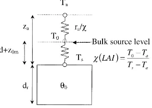
The model has a single-layer interface and a single-bucket representation (Fig. 1). The depth drof the reservoir represents the average value of the maximum depths of the infiltration (i.e. the depth of sharpest decrease in the humidity profile) and drying (i.e. the depth of sharpest increase in the humidity profile) fronts. Time is divided
Fig. 2. Time series of storm/interstorm events.
(Fig. 2) into interstorm and storm events. These two events are periods where water movement is restricted to a combination of evaporation and percolation processes (interstorm) and periods where it is restricted to a combination of runoff and infiltration (storm), respectively.
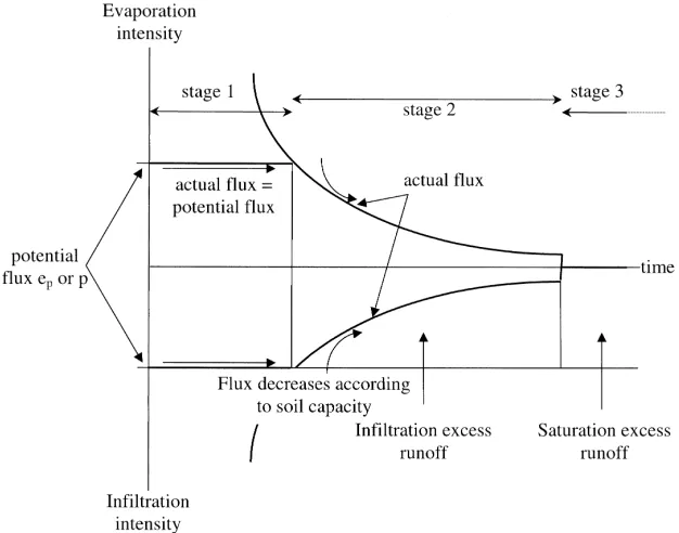
Each storm or interstorm is divided into the well-known three successive stages, defined by Idso et al. (1974) for evaporation but valid for infiltration as well (Fig. 3):
• Stage 1: the water exchange rate is limited by the atmospheric ‘potential’ intensities of rain and potential evap-oration. The bucket is able to release (interstorm) or absorb (storm) water at potential rate. This stage is called ‘atmosphere limited’ or ‘atmosphere controlled’. We suppose that the potential intensity is constant throughout this period.
• Stage 2: the water exchange rate is no longer limited by the ‘drying’ or ‘wetting’ capacity of the atmosphere, and depends only on the capacity of the bucket to release or absorb water. This stage is called ‘soil limited’ or ‘soil controlled’.
• Stage 3: if the bucket water content exceeds saturation or drops below the residual value, water is no longer exchanged.
Mass and energy cycles are related through the calculation of the potential rate and the time of switching from stage 1 to stage 2 during interstorm periods. Contrary to the electrical analogy, where soil and vegetation controls on evaporation are reproduced with the help of empirical surface resistances (allowing for the calculation of real time feedback mechanisms), this time of switching is the only link between the interface and the soil module: the interface imposes the potential rate to the fluxes within the soil, which in turn imposes the actual rate during stage 2.
2.2. The soil module: infiltration and exfiltration capacities
The soil module of the model is built with the following hypothesis: • Soil is homogeneous and does not interact with the saturation zone.
• Water redistribution at the end of each storm or interstorm is immediate and leads to a uniform profile of soil water contentθ0, i.e. a single-bucket value which will be used to describe the water movement during the next storm or interstorm period.
• Water movement in the soil is governed by the quasi-exact analytical solution under the concentration boundary condition of the Richards (1931) equation called ‘capacity’. They are derived from piston flow approximation (Fig. 4): water transfer is described by a moving capillary fringe at variable water content combined with the movement of a piston at constant water content. Whereas the general solution depends on successive flux and concentration boundary conditions, the analytical approximation combines both conditions in a single concen-tration condition through the mean of the Time Compression Approximation (TCA) described later. Evaporation takes place at the surface so that the only transfer occurring within the soil is in the liquid phase. The analytical solution for the infiltration capacity is taken from Green and Ampt (1911) and the so-called exfiltration capacity for evaporation is taken from an inverse Green and Ampt method described in detail by Salvucci (1997). These capacities are similar in form and will thus be described simultaneously in two appended columns:
Darcy’s law applied to the soil surface (exfiltration) or under the saturated piston (infiltration) is
e(z=0)= −D(θ ) ∂θ
where D is the liquid diffusivity, and K is the hydraulic conductivity.
If we assume that the water content profile within the capillary fringe preserves geometric similarity during movement (i.e. the ‘S’-shaped curve of Fig. 4 is symmetrical), and that the space scale characterizing the similarity is zf, the depth of the drying or the infiltration front above or beneath the piston, then there is a single relationship between the water content profile and the dimensionless ratio z/zf, translating into
Fig. 4. Simplified description of the successive profiles of soil water content: top — snapshot at date t, showing the instantaneous fuxes, exfiltration
e and percolation on the left and infiltration i on the right; bottom — after a time lag of dt, showing the cumulative fluxes corresponding to the
movement of the ‘S’-shaped capillary fringe and the rectangular piston, cumulative exfiltration E is represented on the left and infiltration I on the right).
where G and H are unspecified bijective relationships and t is time with origin at the beginning of each storm or interstorm.
After substitution into the Darcy equation, and application of the chain rule, we have (a, b, c and d being unspecified proportionality factors)
e= a
zf(t ) (8a)
i= b
zf(t )+Ksat (8b)
Mass conservation reads (E is the cumulated exfiltration and I the cumulated infiltration)
czf(t )=E+K0t (9a) | dzf(t )=I (9b)
After elimination of zf, e= ac
E+K0t
(10a)
i=Ksat+bd
If we apply the Philip (1957) time series development and identify the first terms
where desorptivity Sdand sorptivity S are
Sd2= 8 (12a) is from Parlange et al. (1985) and (12b) is from Parlange (1975).
By integration (cf. Boulet, 1999), it follows
K0
If t, e, i, E and I are scaled to produce dimensionless variables (‘∼’ superscript),
˜
Then, the capacities e, E, i and I reduce to a form that is independent of the initial or boundary conditions (Haverkamp et al., 1998):
And if we use the Brooks and Corey (1964) retention curve and hydraulic conductivity equations,
θ
2.3. Calculation of potential evaporation
Potential evaporation is deduced from the resolution of the energy balance in potential conditions at the aerody-namic height:
Rnp =Hp+Lep+Gp (22)
The source is supposed to be saturated in potential conditions, and evaporation is expressed by the mean of a surface resistance whose value is the sum of the aerodynamic resistance ra and a minimal stomatal resistance rst minif the surface is vegetated. All fluxes depend on the aerodynamic temperature:
• Net radiation in potential conditions is
Rnp =(1−α)Rg+εs(εaσ Ta4−σ Tsp4) (23)
whereαis the surface albedo, Rg the incoming solar radiation,εa the air emissivity, σ the Stefan–Boltzman constant, Tathe air temperature at reference height,εsthe surface emissivity, and Tspthe surface temperature in potential conditions.
• Soil heat flux is a fractionξof the net radiation:
Gp=ξ Rnp (24)
where Rn, and thus G, can be corrected to account for the vegetation interception in a Beer–Lambert-type relationship:ξ =ξse−0.4LAI.
• Sensible heat flux is
Hp=ρcp
T0p−Ta ra
(25)
• Latent heat flux is
Lep= ρcp
γ
esat(T0p)−ea ra+rst min
(26)
The relationship between the aerodynamic temperature T0p and the surface temperature Tsp is an empirical expression (Chehbouni et al., 1997) function of air temperature and the leaf area index (LAI):
χ= T0p−Ta Tsp−Ta =
1
eυ/(υ−LAI)−1 (27)
whereυis an empirical parameter.
Aerodynamic resistance is derived form a logarithmic wind profile:
ra0=(ln((za−d)/zom)) 2 κ2u
a
(28)
where displacement height d and roughness length zomdepend on vegetation height zvfollowing the ‘rule of thumb’ (Monteith, 1965):d =0.66zvandzom=0.13zv;κ=0.4.
ra0is modified to account for the stability correction (Choudhury et al., 1986): ra=ra0
1
(1+Ri(T0p−Ta))η
(29)
If we perform a first-order development of the energy balance according to the aerodynamic temperature (in a manner similar to the combination equation (Raupach, 1995)), we have
Lep= the radiative–conductive conductance,ga0=1/ra0the aerodynamic conductance without stability correction, and wheregsurf=∆/γ (rst min+ra0)is the total surface conductance without stability correction.
2.4. The Time Compression Approximation (TCA)
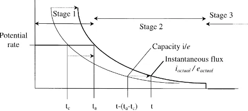
Capacities e and i are analytical solutions of water movement for a soil with a concentration upper boundary condition (θ (z=0)=0 for exfiltration andθ (z =0)=θsatfor infiltration). The TCA allows for the use of the capacities to derive the actual flux when there is a succession of flux and boundary conditions, which is almost always the case in practical situations. It is based on the following hypothesis: the analytical expression of the capacity remains valid during stage 2 but has to be adapted to take into account the amount of water exchanged between the soil and the atmosphere during stage 1. The actual fluxes (written with the ‘actual’ subscript) depend only on the capacity, the cumulative flux exchanged up to that time and the initial water content (Salvucci and Entekhabi, 1994). This hypothesis is equivalent to neglecting the second-order fluctuations (such as meteorological fluctuations) in deriving the instantaneous flux: during stage 1, the actual flux is constant and equal to the potential rate, and during stage 2, it decreases according to the capacity.This hypothesis implies (R and U are unspecified biprojections)
e(t, θ0)=R[E(t, θ0)]⇔eactual(t, θ0)∼=R[Eactual(t, θ0)] (31a) | i(t, θ0)=U[I (t, θ0)]⇔iactual(t, θ0)∼=U[Iactual(t, θ0)] (31b) If we define a ‘compression time’ tcas the time for which the capacity equals the potential rate,
e(tc)=ep (32a)
i(tc)=p (32b)
If we define the ‘time of switching’ tawhen soil begins its control over the instantaneous flux, i.e. the last moment for which the actual rate is equal to the potential rate:
eactual(ta)=ep (33a)
Thus, according to the TCA,
Eactual(ta)∼=E(tc) (35a)
Since the fluxes during stage 2 are decreasing according to the analytical expression of the capacity, the above equality between actual cumulated fluxes and the cumulated capacity is valid as well through the TCA for instantaneous fluxes at any later date:
Fig. 5. The relationship between the capacity and the actual flux according to the TCA.
All expressions remain valid if we replace the dimensional quantities by their corresponding dimensionless values. For instance for tcand ta, Eventually, the mean water content is updated at the end of each interstorm or storm period by solving the cumulated water balance up to that time. It provides the initial water content for the next event (subscript i stands for event number, interstorm or storm): the initial water content for each interstorm is the final water content of the last storm, and vice versa:
Sivapalan and Milly (1989) have shown that the validity of the TCA increases for soil with a highly non-linear diffusivity. It is exact for Green and Ampt type soils (Dooge and Wang, 1993) which show a Dirac mass diffusivity.
2.5. Diurnal cycle reconstitution
Potential evaporation is calculated at each time step of the atmospheric forcing (typically: 1 h) using the meteo-rological data. The average value over the whole interstorm is used in the TCA. The solution of the TCA, the actual exfiltration derived from the exfiltration capacity, is a continuous monotonous decreasing function. It describes the average release of soil moisture in response to an average constant atmospheric stimulation. If we want to unravel the diurnal fluctuations of the energy balance, it is necessary to disaggregate in time the exfiltration capacity which has a typical daily time step. If we suppose that the ratio adaybetween the actual and potential daily evaporation remains valid at smaller time scales, we can relate the instantaneous fluctuations of Le to those of Lep:
Le(t )=adayLep(t ) (45)
Fig. 6. Model algorithm.
ratio of actual exfiltration e cumulated over 1 day and the cumulative value of Lep over the same amount of time:
aday = LP
1 daye
P
1 dayLep
(46)
We can thus impose Le(t )=adayLep(t )in the energy balance to calculate the other fluxes and the simulated surface temperature.
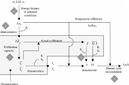
2.6. Model algorithm
The mass and energy balance leading to the latent heat flux for each interstorm (or, similarly, the intensity of infiltration during a storm) is the following (see Fig. 6):
1. The average potential evaporation flux is derived from the available atmospheric forcing and surface parameters. 2. This rate is divided by the corresponding scaling factor (K0for evaporation) to derive the dimensionless potential
rate.
3. Potential evaporation is introduced in the TCA to derive the dimensionless compression time and time of switch-ing, and then the actual dimensionless exfiltration rate.
4. By rescaling the above (i.e. multiplying the dimensionless exfiltration by the proper scaling factor), we simulate the actual exfiltration rate.
Table 1
Values of the main parameters and initial conditions before and after minimization of the distance between the observed and simulated surface temperatures
Symbol θ0,0a Ksat(m/s) mBC θsat ψBC(m) ξ ν dr(cm)
Initial 0.15 4×10⁻⁶ 1.3 0.35 −0.5 0.35 1.5 25
Calibrated 0.12 4×10⁻⁷ 0.5 0.35 −0.9 0.39 2.5 40
aθ
0,0is the initial water content for the whole time series.
3. Application and evaluation of the model for SALSA
3.1. Data used
The data used in this study is taken from a natural pasture site located on the Mexican side of the Upper San Pedro River Basin. It has been instrumented in 1997 as part of the SALSA project (Goodrich, 1994). The objective of the investigation in the Mexican part of the Upper San Pedro basin is to better understand ecosystem function, and manage scarce natural resources by initiating the development and validation of a coupled SVAT and vegetation growth model for semi-arid regions that will assimilate remotely sensed data. Instrumentation was deployed during the summer of 1997 over sparse grass at the Zapata village (31.013◦N, 110.09◦W; see Fig. 1 (Goodrich et al., 2000, this issue)). The soil is mainly sandy loam. A tower has been installed to measure conventional meteorological data (incoming radiation and net radiation at a height of 1.7 m with REBS Q6 net radiometer, wind speed and direction, air temperature and humidity at 6.8 m with the eddy covariance system). Surface temperature was measured with Everest Interscience Infrared radiometers. Measurements of vegetation biomass, water content and leaf area index were made once a week. An eddy covariance system developed at the University of Edinburgh: Edisol (Moncrieff et al., 1997) was used to measure turbulent surface fluxes. The system is made up of a three-axis sonic anemometer manufactured by Gill Instrument (Solent A1012R) and an IR gas analyzer (LI-COR 6262 model) which is used in close path mode. The system is controlled by specially written software which calculates the surface fluxes of momentum, sensible and latent heat and carbon dioxide, from the output of the sonic and IR gas analyzer and displays them in real time. The software performs coordinate rotation on the raw wind speed data and allows for the delay introduced into CO2/H2O signal as a result of the time of the travel down the sampling tube.The climate forcing used in this study covered a period of 19 days. Parameter values are given in Table 1.
3.2. Results
Table 2
Nash efficiency E, root mean square error (RMSE) and bias B between the observed Yobs and simulated Yest fluxes or temperatures after minimizationa
E, RMSE, B Simple SVAT SiSPAT
Ts(◦C) 0.92, 3.01, 0.69 0.76, 2.24, 4.35
Rn(W/m2) 0.99, 15.9,−6.35 0.99, 12.0,−10.4
G (W/m2) 0.82, 30.0, 16.9 0.82, 34.1,−6.5
H (W/m2) 0.82, 37.9, 5.9 0.89, 31.7, 0.9
Le (W/m2) 0.62, 30.3,−5.5 0.47, 42.6, 20.8
aE, RMSE and B are given by
E=1−
" Pi=n
i=1(Yiest−Yiobs)2
Pi=n
i=1(Yiobs−E(Yobs))2
#
, RMSE=
v u u t 1 n
n
X
i=1
(Yiest−Yiobs)2, B=1 n
n
X
i=1
(Yiest−Yiobs).
The ‘bulk’ parameters found by minimization have a lower conductivity and a higher retention capacity. This can be explained by the fact that vegetation, though stressed, is still active and has a negative feedback on water exchange at the surface (effect that is not completely taken into account by the surface resistance in the ‘potential transpiration’ expression).
To check whether the model gives results identical to those of a detailed SVAT model (namely SiSPAT), provided one uses identical parameters, a numerical experiment has been carried out over bare soil for two short-term (a few weeks) and two long-term (1 year) sets of observed climate forcing (Boulet, 1999; Boulet et al., 1999b). Results in terms of cumulated evaporation, runoff and integrated water content over the hydrodynamically active depth match fairly well with the SiSPAT outputs for the long-term time series, whereas for the short term, the integrated water
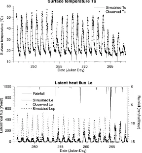
Fig. 8. Simulated and observed latent heat flux and surface temperature.
content over drdiffers greatly between the single bucket and SiSPAT. It shows how sensitive the model outputs are to the specification of dr when the series involves a few numbers of storm or interstorm periods. This sensitivity decreases when this number increases because of the negative feedback of soil moisture over the fluxes.
4. Conclusions
A simple analytical model has been presented and partially validated for a natural grassland in semi-arid area. The scheme offers the following advantages:
• It uses a small number of key parameters representing key processes.
• Its derivatives and integral quantities (such as cumulative fluxes) can be expressed analytically.
• It is suitable (by mean of the non-dimensional quantities) for land surface fluxes scaling. The underlying scaling method will be presented in a companion paper.
But it presents the following drawbacks:
• It uses a flux boundary condition that is averaged in time (which can be a misleading assumption for storm events). • It is a soil-oriented model that can be applied in the case of a short vegetation cover if ‘bulk’ parameters are derived by minimization or if the ‘potential transpiration’ concept is extended (by means of the simple feedback mechanism presented by Monteith (1995) for example). A bare soil version of the model is obtained when setting rst min=0 andχ=1.
Acknowledgements
CONACYT, NASA EOS program (grant NAGW2425), NASA grant W18,997, French Programme National de Télédétection Spatiale and the USDA-ARS Global Change Research Program are gratefully acknowledged. Thanks to Chris Watts, Julio Cesar Rodriguez and Yann Nouvellon for their help during the experiment in Mexico.
References
Braud, I., Dantas-Antonino, A.C., Vauclin, M., Thony, J.-L., Ruelle, P., 1995. A Simple Soil–Plant–Atmosphere Transfer model (SiSPAT) development and field verification. J. Hydrol. 166, 231–250.
Boulet, G., 1999. Modélisation des changements d’échelle et prise en compte des hétérogénéités de surface et de leur variabilité spatiale dans les interactions Sol–Végétation–Atmosphère. Thèse de Doctorat de l’Université Joseph Fourier Grenoble I, Grenoble, France.
Boulet, G., Kalma, J.D., Braud, I., Vauclin, M., 1999a. An assessment of effective land-surface parameterisation in regional-scale water balance studies. J. Hydrol. 217, 225–238.
Boulet, G., Chehbouni, A., Braud, I., Vauclin, M., 1999b. Mosaic versus dual source approaches for modeling the surface energy balance of a semi-arid land. Hydrol. Earth Syst. Sci. 3 (2), 247–258.
Brooks, R.H., Corey, A.T., 1964. Hydraulic properties of porous media, Hydrology paper, 3. Colorado State University, Fort Collins. Brunet, Y., Itier, B., McAneney, K.J., Lagouarde, J.P., 1994. Downwind evolution of scalar fluxes and surface resistance under conditions of
local advection. Part II. Measurements over barley. Agric. For. Meteorol. 71, 227–245.
Brutsaert, W., Chen, D., 1995. Desorption and the two-stages of drying of natural grassland prairie. Water Resour. Res. 31 (5), 1305–1313. Burdine, N.T., 1953. Relative permeability calculation from particle size distribution data. Trans. AIME 198, 71–78.
Camillo, P.J., 1991. Using one- and two-layer models for evaporation estimation with remotely sensed data. In: Land Surface Evaporation. Measurement and Parameterization. Springer, Berlin, pp. 183–197.
Chehbouni, A., Lo Seen, D., Njoku, E.G., Lhomme, J.-P., Monteny, B., Kerr, Y., 1997. Estimation of sensible heat flux over sparsely vegetated surfaces. J. Hydrol. 188/189, 855–868.
Choudhury, B.J., Reginato, R.J., Idso, S.B., 1986. An analysis of infrared temperature observations over wheat and calculation of latent heat flux. Agric. For. Meteorol. 37, 75–88.
Dooge, J.C.I., Wang, Q.J., 1993. Comment on an investigation of the relation between ponded and constant flux rainfall infiltration by Pousslovassilis et al. Water Resour. Res. 27 (6), 1335–1337.
Duan, Q., Sorooshian, S., Gupta, V., 1992. Effective and efficient global optimization for conceptual rainfall-runoff model. Water Resour. Res. 28 (4), 1015–1031.
Eagleson, P.S., 1978a. Climate, soil, and vegetation. 1. Introduction to water balance dynamics. Water Resour. Res. 14 (5), 705–712. Eagleson, P.S., 1978b. Climate, soil, and vegetation. 2. The distribution of annual precipitation derived from observed storm sequences. Water
Resour. Res. 14 (5), 713–721.
Eagleson, P.S., 1978c. Climate, soil, and vegetation. 3. A simplified model of soil moisture movement in the liquid phase. Water Resour. Res. 14 (5), 722–730.
Eagleson, P.S., 1978d. Climate, soil, and vegetation. 4. The expected value of annual evapotranspiration. Water Resour. Res. 14 (5), 731–739. Eagleson, P.S., 1978e. Climate, soil, and vegetation. 5. A derived distribution of storm surface runoff. Water Resour. Res. 14 (5), 741–748. Eagleson, P.S., 1978f. Climate, soil, and vegetation. 6. Dynamics of the annual water balance. Water Resour. Res. 14 (5), 749–764.
Entekhabi, D., Eagleson, P.S., 1989. Land surface fluxes hydrology parameterization for atmospheric general circulation models including subgrid variability. J. Climate 2 (8), 816–831.
Famiglietti, J.S., Wood, E.F., 1992. Effects of spatial variability and scale on areally averaged evapotranspiration. Water Resour. Res. 31, 699–712. Franks, S.W., Beven, K.J., Quinn, P.F., Wright, I.R., 1997. On the sensitivity of the soil–vegetation–atmosphere transfer (SVAT) schemes:
equifinality and the problem of robust calibration. Agric. For. Meteorol. 86, 63–75.
Goodrich, D.C., 1994. SALSA-MEX, a large-scale Semi-Arid Land-Surface-Atmospheric Mountain EXperiment. In: Proceedings of the 1994 International Geoscience and Remote Sensing Symposium (IGARSS’94), Pasadena, CA, 8–12 August, Vol. 1, pp. 190–193.
Goodrich, D.C., Chehbouni, A., Goff, B., MacNish, B., Maddock III, T., Moran, M.S., Shuttleworth, W.J., Williams, D.G., Watts, C., Hipps, L.H., Cooper, D.I., Schieldge, J., Kerr, Y.H., Arias, H., Kirkland, M., Carlos, R., Cayrol, P., Kepner, W., Jones, B., Avissar, R., Begue, A., Bonnefond, J.-M., Boulet, G., Branan, B., Brunel, J.P., Chen, L.C., Clarke, T., Davis, M.R., DeBruin, H., Dedieu, G., Elguero, E., Eichinger, W.E., Everitt, J., Garatuza-Payan, J., Gempko, V.L., Gupta, H., Harlow, C., Hartogensis, O., Helfert, M., Holifield, C., Hymer, D., Kahle, A., Keefer, T., Krishnamoorthy, S., Lhomme, J.-P., Lagouarde, J.-P., Lo Seen, D., Laquet, D., Marsett, R., Monteny, B., Ni, W., Nouvellon, Y., Pinker, R.T., Peters, C., Pool, D., Qi, J., Rambal, S., Rodriguez, J., Santiago, F., Sano, E., Schaeffer, S.M., Schulte, S., Scott, R., Shao, X., Snyder, K.A., Sorooshian, S., Unkrich, C.L., Whitaker, M., Yucel, I., 2000. Preface paper to the Semi-Arid Land-Surface-Atmosphere (SALSA) Program Special Issue. Agric. For. Meteorol. 105, 3–19.
Gupta, H.J., Sorooshian, S., Yapo, P.O., 1998. Towards improved calibration of hydrologic models: multiple and non commensurable measures of information. Water Resour. Res. 34 (4), 751–763.
Haverkamp, R., Bouraoui, F., Zammit, C., Angulo-Jaramillo, R., 1998. Soil properties and moisture movement in the unsaturated zone. In: Delleur, J.W. (Ed.), Groundwater Engineering Handbook. CRC Press, Boca Raton, FL, pp. 5.1–5.50.
Idso, S.B., Reginato, R.J., Jackson, R.D., Kimball, B.A., Nakayama, F.S., 1974. The three stages of drying of a field soil. Soil Sci. Am. Soc. 38, 831–836.
Kim, C.P., Stricker, J.N.M., Torfs, P.J.J.F., 1996. An analytical framework for the water budget of the unsaturated zone. Water Resour. Res. 32 (12), 3475–3484.
Kreiss, W., Rafy, M., 1993. Milieu homogène équivalent pour l’étude des flux de chaleur sol-atmosphère par télédétection. In: Hiérarchies et échelles en écologie. Naturalia Publications, Turriers, France, pp. 285–298.
Moncrieff, J.B., Massheder, J.M., De Bruin, H., Elbers, J., Friborg, T., Heusinkveld, K.P., Scott, S., Soegard, H., Verhoef, A., 1997. A system to measure surface fluxes of momentum sensible heat, water vapor and carbon dioxide. J. Hydrol. 188/189, 589–611.
Monteith, J.L., 1965. Evaporation and the environment. In: The State and Movement of Water in Living Organisms, Proceedings of the 19th Symposium, Soc. Exp. Biol., Swansea. Cambridge University Press, Cambridge, pp. 205–234.
Monteith, J.L., 1995. A reinterpretation of stomatal responses to humidity. Plant Cell Environ. 18, 357–364.
Norman, J.M., Kustas, W.P., Humes, K.S., 1995. Source approach for estimating soil and vegetation energy fluxes in observations of directional radiometric surface temperature. Agric. For. Meteorol. 77, 263–293.
Olioso, A., Taconet, O., Ben Mehrez, M., Nivoit, D., Promayon, F., Rahmoune, L., 1995. Estimation of evapotranspiration using SVAT models and surface IR temperature. In: Proceedings of IGARSS’95, Florence, Italy, 10–14 juillet 1995, Vol. 1, pp. 516–518.
Parlange, J.Y., 1975. On solving the flow equation in unsaturated soils by optimisation: horizontal infiltration. Soil Sci. 122, 236–239. Parlange, J.Y., Vauclin, M., Haverkamp, R., Lisle, I., 1985. Note: The relation between desorptivity and soil-water diffusivity. Soil Sci. 139,
458–461.
Philip, J.R., 1957. The theory of infiltration. Soil Sci. 1 (7), 83–85.
Press, W.H., Teukolsky, S.A., Vetterling, W.T., Flannery, B.P., 1992. Numerical Recipes in FORTRAN. The Art of Scientific Computing, 2nd Edition. Cambridge University Press, Cambridge, 962 pp.
Raupach, M.R., 1995. Vegetation–atmosphere interaction and surface conductance at leaf, canopy and regional scales. Agric. For. Meteorol. 73, 151–179.
Richards, L.A., 1931. Capillary conduction of liquids through porous media. Physics 1, 318–333.
Salvucci, G.D., 1997. Soil and moisture independent estimation of stage-two evaporation from potential evaporation and albedo or surface temperature. Water Resour. Res. 33 (1), 111–122.
Salvucci, G.D., Entekhabi, D., 1994. Equivalent steady soil moisture profile and the time compression in water balance modeling. Water Resour. Res. 30 (10), 2737–2749.
Sivapalan, M., Milly, P.C.D., 1989. On the relation between the time condensation approximation and the flux–concentration relation. J. Hydrol. 105, 357–367.
Soer, G.J.R., 1980. Estimation of regional evapotranspiration and soil moisture conditions using remotely sensed crop surface temperature. Remote Sens. Environ. 9, 27–45.
Taconet, O., Olioso, A., Ben Mehrez, M., Brisson, N., 1995. Seasonal estimation of evaporation and stomatal conductance over a soybean field using surface infrared temperature. Agric. For. Meteorol. 73, 321–337.