A GENERIC PROBABILISTIC MODEL AND A HIERARCHICAL SOLUTION FOR
SENSOR LOCALIZATION IN NOISY AND RESTRICTED CONDITIONS
S. Ji a, b, *, X. Yuana
a School of Remote Sensing and Information Engineering, Wuhan University, Wuhan 430049, China – (jishunping, yuanxx) @whu.edu.cn
b RSISE, Australian National University (ANU), Canberra ACT 2600, Australia
Commission I, WG I/3
KEY WORDS: Generic Probabilistic Localization Model, Bundle Adjustment, Kalman Filtering, Particle Filtering
ABSTRACT:
A generic probabilistic model, under fundamental Bayes’ rule and Markov assumption, is introduced to integrate the process of mobile platform localization with optical sensors. And based on it, three relative independent solutions, bundle adjustment, Kalman filtering and particle filtering are deduced under different and additional restrictions. We want to prove that first, Kalman filtering, may be a better initial-value supplier for bundle adjustment than traditional relative orientation in irregular strips and networks or failed tie-point extraction. Second, in high noisy conditions, particle filtering can act as a bridge for gap binding when a large number of gross errors fail a Kalman filtering or a bundle adjustment. Third, both filtering methods, which help reduce the error propagation and eliminate gross errors, guarantee a global and static bundle adjustment, who requires the strictest initial values and control conditions. The main innovation is about the integrated processing of stochastic errors and gross errors in sensor observations, and the integration of the three most used solutions, bundle adjustment, Kalman filtering and particle filtering into a generic probabilistic localization model. The tests in noisy and restricted situations are designed and examined to prove them.
* Corresponding author
1. INTRODUCTION
In classic photogrammetry, bundle adjustment based on least square methods is the main technic for the image or called sensor or platform localization. The advantages and disadvantages are both explicit: global optimum, rigorous, capable both to real time/off time processing, but short in requiring accurate initial values, adequate GCPs and outlier free. In some cases, especially when close range photogrammetry is involved, those prerequisites are difficult to meet. For example, it is hard to make enough GCPs for short-baseline imagery acquire from ground mobile mapping system (MMS) especially in urban street. Another case is, if imagery from an unmanned aerial vehicle (UAV) meets water surface or forest with undistinguishable textures, the gross errors in image matching or a complete failed matching will destroy the automatic triangulation processing.
If turning back to the early days, we could find a plenty of articles dealing with platform localization especially self-localization in control, navigation and robotics society. The main tool is called extended Kalman filtering (EKF) (Bishop and Welch 2001), which infer only the current best status. It means it’s not a global solution (a rarely used statistic EKF is equivalent to bundle adjustment in nature). However, EKF need less perquisites than bundle adjustment. It requires the accurate initial status of only the first image. If there are only a few GCPs or not even one, it can still give a not too bad solution. However, EKF and bundle adjustment, both requiring observations obeying the Gaussian independent distributions, cannot deal with the (plenty of) outliers themselves. A RANSAC (Fischler and Bolles 1981) based technic can detect easily the outliers in stereo image matching, but almost
impossible in bundle adjustment in which hundreds and thousands of parameters may be involved. Data snooping or gross error detection methods based on posteriori variance estimation still cannot handle the situation with a large number of outliers (e.g., more than 50%). The same rule is suitable for EKF and other so called robust methods as ||L||1 (bundle adjustment can be looked as ||L||2).
In the 1990s particle filtering was gradually applied to sensor localization in the field of robotics, especially in its branch study, simultaneous localization and mapping (SLAM) (Thrun et al. 2001). The particle filtering is originally an alternative to EKF, but with more efficient and less memory space (Thrun et al. 2004). However, it has a strong enough property, that it doesn’t require Gaussian independent assumption anymore. It can deal with non-Gaussian observations, considering that even outliers can also be one type of special observations. In theory, particle filtering itself is a robust method against outliers and does not require extra gross error detection methods to be imbedded. Another property of particle filtering is, it can handle the situation with no initial status, for example, a robot kidnaping problem.
The three mainstream technics, bundle adjustment, EKF and particle filtering, can compensate each other theoretically when we meet a special difficult localization problem considering their different properties.
However, they are relatively independent. In this paper the first thing is integrating them under a uniform framework, which called a probabilistic localization model, based on Bayes rule and Markov chain assumption (Ji et al. 2015). In turn, the three methods, as different solutions to the generic model, will be rediscovered.
The next thing is to prove that a hierarchical strategy, based on the generic model with the three solutions, is more robust to a challenging localization problem than only a solution, say, bundle adjustment. We design two tests, and the one is imagery localization from a UAV, with unmatchable images; the other is MMS localization with panoramic imagery, where no GCP available and only a geo-referenced orthogonal aerial images. The former test will be handled with first EKF and then a global bundle adjustment, and the last with first particle filtering and then bundle adjustment.
2. A GENERIC PROBABILISTIC LOCALIZAITON MODEL AND ITS SOLUTIONS
2.1 A generic probabilistic localization model
The probabilistic model for a sequential localization problem can consist of two types of constraints, observations and motions. The observation values except for motion are called obeying observation models, including co-linearity equations, GPS observation equations et al. While motion models, representing the motion between adjacent images, can often be acquired from a gyro, and a real or visual odometry. We use St
and Gt respectively for all the observations and motion
constraints of the vehicle up to time t, St and Gt respectively for
only time t. Let Lt represent the current pose, and Lt represent
the entire path up to t. Conditioned on the two constraints, the posterior p(Lt|St,Gt) or so called belief Bel(Lt) should be
maximized to achieve an optimal solution. According to Bayes’ rule, we have
t t| t, t
= | t, t, t1
t| t1, t
t
Bel L p L S G p S L G S p L S G (1)
In (1), η is a normalized constant equal to p(St|St-1,Gt)-1.
Typically, the observations (e.g., tie points) St-1 are independent of each other, and can be omitted in p(St|Lt,Gt,St-1). Assuming
the trajectory be represented as a probabilistic Markov chain (Montemerlo 2003), where the previous poses are independent of the current system status if the current pose is known, Lt-1
Eq. (3) can be further written as
problem where observations and motions are independent and the motion trajectory satisfies a Markov chain.Please note that this model is suitable to handle significant noises for a localization problem, since it has no assumption on the distribution of the observations as required commonly. Further, the recursive nature of the model allows highly noisy observations be gradually filtered out by taking advantage of the successive and relatively accurate motion constraints, when a direct global solution is almost impossible.
2.2 The three solutions to the model
The special pose estimation methods, bundle adjustment, Kalman filtering and particle filtering, can be rediscovered when additional assumptions are introduced to the generic model Eq. (4), because they share the same probabilistic basis: estimate the posterior distributions over poses under certain independence assumptions.
2.2.1 Bundle adjustment solutions
Let St, Lt, and Gt be the image coordinates, exterior orientation
elements, and correspondent world coordinates, respectively, observation model p(St|Lt,Gt) then becomes the posterior of
co-linearity functions and p(Lt|Lt-1,Gt) the relative orientation.
Suppose the observations following Gaussian distributions, we can deduce the quadratic form from (4)
expectation and covariance of the co-linearity, and relative orientation or called motion model in robotics, respectively. Realizing the two Mahananobis distances, Eq. (5) can be solved by an relative bundle adjustment method that integrates relative orientation constraints into bundle adjustment solutions (D. Sibley and Mei 2009; G. Sibley et al. 2010), or a traditional one just disregarding the motion model.
2.2.2 Extended Kalman filtering solutions
The posterior p(Lt| Lt-1,Gt) is predictions expressed by motion
model u(Lt-1,Gt) as Eq. (6) where Qt,
P
ˆ
t and Ft are themeasurement noise of Gt, predicted covariance matrix and
Jacobians of motion model respectively. The posterior of observation model p(St|Lt,Gt) is innovations expressed by (7)
where st, Ht, vt and Dt represent observations, Jacobians of the
observation model, the measurement residual and covariance, respectively. The gain Kt and the final estimations of the current
position Lt and covariance Pt are expressed in (8). Note that the particles to discretize the continuous posterior Bel(Lt), similar to
Markov chain Monte Carlo (MCMC). As in Eq. (9), the posterior is represented by a random collection of weighted particles that approximates the target distribution, where
,[ ]
1, ,2 ,
t i i i i
t
l l l l is the hypothesized trajectory of the i-th
particle up to time t, and the corresponding weights or named
importance factors ,[ ]
1, 2, ,
t i i i i
t
w w w w determine its
importance. Thus, the poses lt,[j] are selected when j-th particle win the maximum weights.
, ,
, , 1, 2, ,
t i t i t
Bel L l w i m (7)
After the posteriors are discretized, classic PF solutions can be implemented. The recursive update consists of three steps:
(1) Draw i1 t
l from the previous weighted particle set which represents Bel(Lt-1).
(2) Sample new particle i t
l according to the motion model:
i t
l ~ p(Lt| lit-1, St-1,Gt). Now the new particle follows a joint probability: p(Lt|lit-1,St-1,Gt) × Bel(Lt-1), which is also called proposal distribution.
(3) According to Eq. (4), the importance factor
w
ti is assigned to the quotient of the target distribution Bel(Lt)and the proposal distribution, i.e., ηp(St|
l
ti,Gt), where η isa constant. Finally, the largest j t
w indicates the solution
lt,[j].
2.3 A simple simulated comparison of the three solutions
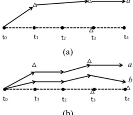
The situation with plenty of outliers which hard to be eliminated is perhaps the most difficult case for an automatic localization application. Here we give a simulated example. Figure 3 graphs the performances of the three solutions using a simulated trajectory corresponding to the cases in Figure 1, where dashed line with five black dots (as images) is the referenced trajectory and also the predicted trajectory of motion model of a vehicle. However, there are some obvious errors in GCPs at time t1 and t3. There are even two GCP candidates (considering the GCPs are obtained from matching images to a geo-referenced maps) in t3 but the candidate above with more confidence. In Figure 1(a), the estimated trajectory a obtained from bundle adjustment is far from the reference path due to GCP errors. Figure 1(b) depicts visible offsets from the reference for two paths a and b derived by EKF, where path a
has higher weights for GCPs and path b has higher weight for the motion model. Figure 1(c) is the result of particle filtering, where the diversity of particles and multi-hypothesis tracking guarantees that path c wins with the greatest confidence. Although what presented in Figure 1 is a simulation, we intend to demonstrate that, PF based methods are superior to bundle adjustment and EKF in noisy situation.
(a)
(b)
(c) Figure 1. Performance of three solutions under a simulated
noisy environment.
3. A HIERARCHICAL SOLVING STRATEGY FOR
OPTICAL MOBILE CAMERAS
Although localization problem with other types of sensors, such as laser, can also be solved with the generic probabilistic model and one of its solutions, we focus on optical cameras in this paper. Further, we only focus on the ordinary situation that the optical images are obtained by a mobile platform, a UAV, aerial photography aircraft or MMS. The localization problem with independent photos from crowd sources, such as the famous “building Rome in a day”, is not considered, for those cases lack of the meaning of motion model, and may be only suitable to bundle adjustment.
3.1 Motion models
For optical images the most popular method to obtain motion model is using visual odometry, which is similar to traditional relative orientation. In this section, we first deduce the motion model in probabilistic manner and then extend it to adapt the situation that image matching failed.
The posterior p(Lt|Lt-1,Gt) in Eq. (4) called motion model, which
describes the distribution of the current pose conditioned on the last pose and the current motion parameters.
First of all, any correspondence finding methods, such as SIFT (Lowe 2004) or cross correlation can be applied to obtain enough correspondences between the adjacent images, typically followed by a gross error detection process with RANSAC (Fischler and Bolles 1981) or posteriori variance estimation. Then, sequential relative orientation is carried out with the remained tie-points. The sensor model and the relative orientation model depend on the special cameras be used. In this paper, we use two cameras, a traditional Cannon camera on UAV with a common pinhole model and a panoramic camera, Ladybug 3, on MMS, whose model can be found in (Shi et al. 2013). Third, align the relative orientation parameters to the world coordinate system by fixing the first image’s pose to zero vector or setting it to the approximate geo-referenced values. Let Rt and Tt represent the pose to the world coordinate, and Rt -1,t and Tt-1,t represent the incremental pose. The current position
l is obtained by:
l = Lt-1 + Rt-1,tTt-1,t (10)
where Lt-1 = (xt-1yt-1zt-1) represents the camera position in time
t-1. Thus, a motion model with six parameters <xt-1,t, yt-1,t, zt-1, φt-1,t, ωt-1,t, κt-1,t> can be employed, and each parameter is
considered following a Gaussian distribution, with known co-variance matrix from relative orientation. L0 is the coordinates of the first image.
Let the corresponding accuracy of pose parameters represented by δ, thus the motion model follows a Gaussian distribution:
p(Lt| Lt-1,Gt)~N(l,δ) (11)
However, it perhaps appears in mind that not all the relative orientation has a good solution due to an imperfect matching
with few correspondences remained or a totally failed one, caused by specular reflection, lacking of features or repeated pattern textures. In that case, a traditional automatic triangulation would be interrupted and usually manual intervention be required.
In this paper, we utilize a smooth-driving assumption, that Lt
can be obtain by the relative orientation parameters at time t-2 or earlier with correct relative orientation. Thus,
l = Lt-1 + Rt-2,t-1T t-2,t-1 (12)
And set δto a large value with prior knowledge the same time. when strips form block or GCPs are introduced, the large uncertainty could be supressed largely then.
Thus a motion model is not only a relative orientation, but a more general probabilistic model with more flexibility.
3.2 Observation models
Sensor model, typically the collinear equations, is the main observation model of a traditional bundle adjustment. In the generic probabilistic localization framework, we call posterior
p(St|Lt,Gt) in Eq. (4) observation models, which remains the
same meaning in a large part but with some small extensions. Any observations from GCPs, GPS or other relative geometrical constraints etc., with their own models, all contribute to the overall observation models. In this paper, collinearity, GPS observations and GCPs from an ortho-image are involved. We first discuss GCPs.
3.2.1 observation models of noisy GCPs
We miss the simple case that those traditional, high accuracy GCPs are obtained from manual fieldwork that obey collinearity. Here, GCPs for locating MMS images are obtained from matching the MMS images to the geo-referenced orthogonal images or maps. The image center is then geo-located after a successful match. For convenience, we just set the z-coordinates to a constant since the images were obtained from a flat road. Under the best conditions, the GCPs are all correct. However, it is almost impossible. First, we should geometrically rectify the MMS images to orthographic projection. Any object that is high than the road surface would cause a rectification error. Second, shadows, moving cars, occlusions all contribute to unpredictable changes between MMS images and ortho-image. The truth is the matched GCPs will be full of gross errors, which cannot guarantee a successful bundle adjustment or EKF as observations.
A better strategy looks those GCPs as with hypothesis property, that is, matching can be right or wrong. Naturally MCMC based particle filtering methods is more suitable in this situation. Here, Gt can be ignored if L
t is known since we only match the
image center. Then the specific form of p(St|Lt) is expressed by
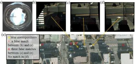
multi-source matching between ground image sequence and ortho-image. First, all the panoramic images (Figure 2(a)) after relative orientation are orthogonally rectified assuming a flat road surface. Further, ten rectified images are stitched into a larger image patch close to a square of about 10 m x 10 m, as shown in Figure 2(b-d). In order to improve the stitching accuracy a bundle adjustment every 10 images can be performed before.
Figure 2. Matching difficulties and the multi-hypothesis nature.
Second, multi-hypothesis multi-source image matching is carried out. According to the motion model Eq. (11), we can sample the current pose Lt from this distribution, and look each
pose a particle. each particle in the ortho-image (Figure 2(e)), along with its neighbourhood, as search image, is matched to the rectified panoramic image (reference image). Classic correlation technology rather than advanced feature matching is more suitable, if the image patches are too small to extract adequate features. A rotation invariant strategy can be used to resist big rotation.
Third, for each particle i, correlation generates a set of correlation coefficients containing a maximum one cmax, and corresponding pixel position lmax. Regard it the only valid particle. That means the number of particles always equals to samples, a constant number as in most PF-based methods. A candidate with cmax above a given threshold, e.g., 0.3, are regarded as invalid. Then the observation model for the matched GCPs is then defined as follows:
max
( | )
i i
t
w p S l c (12) under the normalization constraint ∑iwi = 1.
3.2.2 observation models of collinearity
Both Tie-points and manual GCPs satisfy collinearity. These tie-points are usually correct for they have survived from image matching, gross error elimination, and even local multiple-ray intersection. We model the tie-points and manual GCP observations as Gaussian distributions
p(St|Lt,Gt) ~ N(s,δ) (13)
Here s = g(Lt, Gt) is the calculated image point coordinates from
the collinear equation g(·), and δ is its accuracy respected to the image point (x, y).
3.2.3 observation models of GPS
GPS or GNSS observations should be considered separately according to different situations. The GPS antenna on a UAV or photography aircraft is seldom blocked and can receive signals with better accuracy. While mounted on a MMS, GPS signals are often unlocked by canyon effects or Multipath effects especially in urban streets.
For the case of UAV platform, the GPS observations can be modelled as obeying Gaussian distributions,
p(St|Lt,G) ~ N(s,δ) (13)
Here G, usually a function constant to time t, reflects the geometrical relations between GPS observations St and the
camera pose Lt. Typically,
s = Rtd + Tt (14)
where d is the constant offset between the camera center and phase center of GPS antenna. Rtand Tt are rotation matrix and
translations of exterior orientation elements, retrieved from Lt.
And the accuracy δ could be set with experience.
For the case of a MMS in noisy street environments, GPS signals may be with many blunders, making a global bundle adjustment impossible. The better way may use EKF, still regarding each observation obeying Gaussian distribution, but setting its weight with the consistency to consecutive motion models.
3.3 The hierarchical solving strategy
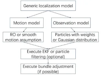
After modelling both observation and motion models, the two essential parts for a mobile platform localization, we can deduce the hierarchical structure of solving methods considering both the random errors and gross errors. As shown in Figure 3, if gross errors exist in motion models, a smooth motion assumption is utilized to construct a Gaussian distributed motion model but with less accuracy; otherwise just calculate the model from relative orientation. If gross errors exist in observations, e.g., GCPs or GPS, there are two strategies. if you can guess the weight of each observation approximately, model it as a Gaussian distribution, otherwise model it as particles with their own weights. At last, solving the generic probabilistic model with EKF or particle filtering if a direct bundle adjustment impossible, depending on the special situation. And bundle adjustment usually be applied the final to achieve perhaps a better global result.
Figure 3. The hierarchical strategy for solving the generic localization model
4. EXPERIMENTS
4.1 Text design
Two tests are designed with special challenging situations. The first dataset is image series obtained from a UAV. However, there are some tie-point extraction troubles that some images were missing, as shown on Figure 4. It may be an impossible task for a traditional triangulation procedure. The other dataset is panoramic image series obtained from a ground MMS. The trajectory was selected in a complex street environment with moving vehicles, occlusions, and shadows.
The data pre-processing of the first dataset is simple: just manually measuring the image coordinates of the 10 GCPs. Set δ to the accuracy of a successful relative orientation in pixels; otherwise, set it to ten percent of the image width.
The pre-processing applied to the second dataset is more complicated. The predicted trajectory, consisted of 2,410 panoramic images with an interval of about 1 m, was initially aligned to the first GPS observations after sequential relative
orientation and local bundle adjustment, shown as yellow line in Figure 5. All the panoramic images were then ortho-rectified and every 10 images are stitched to generate image patches about 10×10 m2 as in Figure 2. The geo-referenced information is an aerial orthogonal image with a ground resolution of 0.2 m and localization accuracy of 0.5 m. The check points are obtained from the processed GPS/IMU joint observations with an accuracy of better than 0.1 m and is shown as the blue trajectory in Figure 5. The required parameters in particle filtering method are set as: particle number is 100; the accuracy of motion model δis 2.00 m (10 pixels), which is also applied to EKF.
4.2 results
4.2.1 The first test
The first UAV test data consist of 4 strips 64 images, whiles some images (in white) were missing. This situation may also be regarded generally as a tie-point extraction problem caused by ill image matching.
Table 1 shows the solving strategies of a direct aerial triangulation of first relative orientation (RO) and then bundle adjustment (direct BA), and our hierarchical solution with first EKF and later a bundle adjustment. With a flexible motion model, the large uncertainty (once reaching more than 1000 pixels) cause by image missing can be reduce to normal level (6.65 pixels) after that missing parts are revisited.
In Table 1 the DXYZ means the 3D accuracy of GCPs, and RMS
means the residual mean square error. It can also be noticed that, the EKF only gives a proximately solution and the following bundle adjustment with the initial values supplied by EKF can guarantee much better accuracy.
Figure 4. the UAV test with missing images
Table.1 results of different solutions (pixels) Method RMS Max DXYZ Min DXYZ
RO / / 0.00
Direct BA / / /
EKF 6.65 4.21 2.23
BA after EKF 0.51 1.54 0.01
4.2.2 The second test
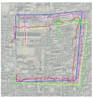
In Figure 5 the yellow line is the predicted trajectory after sequential relative orientation and local bundle adjustment. The red is the reference trajectory obtained from GPS/IMU with 0.1 m accuracy. The blue line is the result of particle filtering. From the “truncated” indicates that the last section in full shadows were removed.
Table.2 check of the localization accuracy
Method DX DY DXY Max
DXY
Min
DXY
RO 43.20 72.00 80.97 167.93 0.01
BA / / / / /
EKF(best) 28.65 17.35 33.49 101.19 0.00 PF(whole) 0.36 0.45 0.57 14.31 0.01 PF(truncated) 0.23 0.39 0.41 4.20 0.01 BA after PF 0.21 0.37 0.39 3.89 0.01
Figure 6 are results of EKF with different weight ratios k0 (green: k0 = 0.1, red: k0 = 1; pink: k0 = 10; white: k0 = 100) between motion models and observations. Obviously, the GCPs obtained from matching are high noisy and cannot guarantee a good EKF result. The same rule applies to bundle adjustment, which were totally failed. Only particle filtering with multi-hypothesis itself can realize an accurate localization.
We then applied the remained good GCPs after particle filtering to a global bundle adjustment with additional flat road surface assumption. This time the bundle adjustment converged to a result that just as good as or only a slightly better than the particle filtering method. The detailed numerical values and comparison are shown in Table 2.
Figure 5. results of particle filtering method
Figure 6. results of EKF method
4.3 Conclusions
In this paper, we introduce a generic probabilistic model for platform localization with optical images. Based on the model, three mostly used solutions, bundle adjustment, EKF and particle filtering, are rediscovered. Further, a hierarchical framework, combining the three methods under the generic model, are proposed. With two datasets under noisy situation, we proved that, the hierarchical framework can handle these situations easily which were extremely challenging to a traditional bundle adjustment.
Except the examples in this paper, the generic model and the hierarchical framework can be further explored to other platforms as satellites, sensors as laser or LiDAR, and difficult situations as noisy GPS supported localization.
ACKNOWLEDGEMENTS
This work was jointly supported by the National Key Basic Research Program of China (2012CB719902), the National Natural Science Foundation of China (41471288, 61403285), and the National High-Tech R&D Program of China (2015AA124001).
REFERENCES
Bishop, G., Welch, G., 2001. An introduction to the Kalman filter. TR 95-041, Department of Computer Science, University of North Carolina at Chapel Hill Chapel Hill, pp. 1-16.
Fischler, M., Bolles, R.C., 1981. Random sample consensus: a paradigm for model fitting with applications to image analysis and automated cartography. Communications of the ACM, 24(6), pp. 381-395.
Ji, S., Shi, Y., Shan, J., Shao, X., Shi, Z., Yuan, X., Yang, P., 2015. Particle filtering methods for georeferencing panoramic image sequence in complex urban scenes. ISPRS Jounal of
Photogrammetry and Remote Sensing. 105 (2015), pp. 1-12.
Lowe, D.G., 2004. Distinctive image features from scale-invariant keypoints. International Journal of Computer Vision
60(2), pp. 91-110.
Montemerlo, M., 2003. Fastslam: A factored solution to the simultaneous localization and mapping problem with unknown data association. Robot. Report CMU–RI–TR–03–28, Institute of Carnegie Mellon University.
Shi, Y., Ji, S., Shi, Z., Duan, Y., Shibasaki, R., 2013. GPS-supported visual SLAM with a rigorous sensor model for a panoramic camera in outdoor environments. Sensors 13(1), pp. 119-136.
Sibley, D., Mei, C., 2009. Adaptive relative bundle adjustment.
Robotics: science and systems 220(3), pp. 1-8.
Sibley, G., Mei, C., Reid, I., Newman, P., 2010. Vast-scale outdoor navigation using adaptive relative bundle adjustment.
The International Journal of Robotics Research 29(8), pp.
958-980.
Thrun, S., Fox, D., Burgard, W., Dellaert, F., 2001. Robust Monte Carlo localization for mobile robots. Artificial
Intelligence 128(1-2), pp. 99-141.
Thrun, S., Montemerlo, M., Koller, D., Wegbreit, B., Nieto, J., Nebot, E., 2004. Fastslam: An efficient solution to the simultaneous localization and mapping problem with unknown data association. Journal of Machine Learning Research 4(3), 380–407.