Combining geostatistics and flow simulators to
identify transmissivity
Chris Roth
a ,*, Jean-Paul Chile`s
a& Chantal de Fouquet
b aBRGM, Avenue Claude Guillemin, BP 6009, 45060 Orle´ans Cedex 2, France b
Centre de Ge´ostatistique, 35 rue St. Honore´, 77305 Fontainebleau, France
(Received 15 November 1996; revised 24 April 1997; accepted 4 June 1997)
The reconstruction of the transmissivity field from the more numerous experimental hydraulic head data, an inverse problem, remains the focus of continuing stochastic-based research. The difficulty of this problem arises not only from the complexity of the diffusion equation that links the two variables, but also from taking into account the physical aspects of the site under study; e.g. the boundary conditions, the effective recharge, and the geology. In practical applications, the validity of purely analytical techniques proposed to date is limited by certain simplifying assumptions, like the linearization of the flow equation, made in order to obtain a solution. For this reason, a hybrid methodology combining geostatistical techniques with deterministic numerical flow simulators is proposed. This combination allows the numerical calculation of the direct and cross covariances needed to cokrige the transmissivity from both the transmissivity and hydraulic head data. The flexibility of numerical flow simulators takes away the need for the simplifying assumptions of analytical techniques to apply the proposed methodology.q1998 Elsevier Science Limited. All rights reserved
Key words: geostatistical simulation, inverse modelling, transmissivity, hydraulic head, flow simulators, cokriging, numerical covariances.
1 INTRODUCTION
The problem treated in this paper is one of mapping trans-missivity. That is to obtain the most likely transmissivity value in the field that allows us, for example, to localise zones of high or low transmissivity. This is an estimation (by cokriging) problem and not one of simulation, which is more appropriate when one wishes to reproduce the observed head field, for example, for later velocity or trans-port calculations. A certain number of techniques1–3 have recently been proposed for this simulation problem.
When estimating transmissivity by cokriging, a suitable covariance model must be developed. For about 15 years, researchers have been trying to stochastically incorporate the diffusion equation, in its analytical form, in the transmissivity–hydraulic head covariance model. While a complete review of the techniques proposed to date has recently appeared4, a summary of the main types of
approach is provided here. Spectral analysis5was the first approach used to link the transmissivity and hydraulic head covariances. The method of small perturbations was used to provide a first-order solution of the diffusion equation, the head perturbation being expressed as a function of the log-transmissivity perturbation. The framework of this work was that of two-dimensional steady-state groundwater flow with zero effective recharge for which boundary con-ditions are ignored, or equivalently assumed to have no influence on the hydraulic head field.
Other techniques, such as maximum likelihood pro-cedures6,7or intrinsic random function theory8, were subse-quently applied to the same problem. However, while the methodology changed, the basic framework of the problem and the approximations made have remained more or less the same. Some generalisations, such as including a non-constant mean transmissivity9 or a constant effective recharge term10, have been made. A recent work11 intro-duces both a variable effective recharge and a fixed con-figuration of boundary conditions that is applicable in practice when the natural aquifer form is approximately
Printed in Great Britain. All rights reserved 0309-1708/98/$19.00 + 0.00
PII: S 0 3 0 9 - 1 7 0 8 ( 9 7 ) 0 0 0 1 9 - 5
555
rectangular. So, while progress is being made towards a general working framework, the use of a first-order solution of the diffusion equation remains a very limiting constraint in practical applications. While it has been suggested12that a first-order solution is valid for a log-transmissivity vari-ance of up to 1, in practice13this variance commonly attains values between 2 and 3.
To remove the limiting assumptions associated with analytical approaches, models based on the mixture of geo-statistics and numerical flow simulator results have been proposed. Two different techniques14,15based on a similar idea have been proposed. The line of thinking is to krige an initial transmissivity field that is then iteratively modified until the numerical flow simulator results correspond with the observed head values. The modification of the initial field depends on the number, the location and the value of the fictitious transmissivity data added to the actual experi-mental data set. Another approach16is to develop a covar-iance model that links the log-hydraulic conductivity to the head-squared because, as stated by the authors, ‘‘the equa-tions of flow are simplified by the use of the head-squared instead of the head.’’ Monte Carlo simulations are used to express the head-squared covariance and the cross covariance between the head-squared and the log-hydraulic conductivity as a piece-wise linear function of the parameters defining the log-hydraulic head covariance. These parameters are then obtained by a maximum likeli-hood procedure under a multi-Gaussian hypothesis that is justified for weakly variable log-hydraulic conductivity. The resulting analytical covariances are used to cokrige the hydraulic conductivity and a constant effective recharge is finally calibrated to the cokriged field as the value that leads to the best experimental fit for the head-squared variable.
A different technique, also based on several Monte Carlo simulations, is proposed in this paper. Given the transmis-sivity covariance model, a series of transmistransmis-sivity fields is simulated and the corresponding head fields obtained by a numerical flow simulator. However, the form of the hydraulic head itself is largely determined by the boundary conditions, the effective recharge and the mean transmissiv-ity of the aquifer, and as such masks the influence of the smaller-scale head variations which result from the local variations of the transmissivity. So, to extract the maximum amount of information from the data, a covariance model linking the log-transmissivity to the head variation will be developed. So the parallel series of fields, or what we shall termjoint flow simulations, are used to numerically calcu-late the direct and cross covariances that lead to the cokrig-ing of the transmissivity field from both the transmissivity and head variation data. The steps of the method are: (1) defining the transmissivity variogram from experimental data and geostatistically simulating a large number of trans-missivity fields; (2) obtaining the corresponding head fields by numerical flow simulator; (3) calculating the mean head field and, in turn, the resulting series of head variation fields; (4) numerically calculating the required direct and cross
covariances for all pairs of points; and (5) estimating the log-transmissivity by cokriging from the log-transmissivity and the head variation data, using the numerical covariances.
Given the numerical-based character of the technique proposed, the convergence rate of the numerical covariances and the positive definiteness of the resulting numerical cok-riging covariance matrix will be discussed in some detail. The method will be applied to a sandy aquifer from the north of France for which special attention is paid to the vario-graphic analysis of the log-transmissivity given that the measurements taken are neither punctual nor accurate.
2 JOINT FLOW SIMULATIONS
2.1 Geostatistical transmissivity simulations (step 1)
With a view to the case study later treated, the scalar trans-missivity is modelled as being lognormally distributed and stationary over the aquifer. The mean and variance of the normally distributed log-transmissivity lnT, are denoted by
mandj2, respectively. The transmissivity can be geostatis-tically simulated once its covariance model has been fixed from either the experimental data or from other aquifers presenting similar hydrodynamic characteristics. However, given the skewness of the experimental data, there is a greater likelihood of having a few very large values that may obscure the inference of a covariance model from the experimental covariance. Working in terms of the Gaussian log-transmissivity minimizes the sensitivity of the experi-mental covariance. Moreover, the convergence rate of Gaussian simulations is orders of magnitude higher than that of the equivalent lognormal variable17 because of the influence of the high values that make up the tail of the lognormal distribution. Hence, choosing the first variable of interest as lnTlimits the number of simulations needed for the numerically calculated covariances to converge. Working with lnTor with its fluctuations about the constant meanmleads to the same result.
The transmissivity fields are non-conditionally simulated using a method based on the discrete spectral density18, which ensures the normality of the probability law of lnT, and hence the lognormality of the reconstructed trans-missivity. These simulations reproduce the experimental covariance and histogram. If we had used a series of con-ditional transmissivity simulations, the simulated value at the data points is always equal to the experimental value itself. So the numerical covariance between experimental points, calculated as the covariance between two constant values, is equal to zero. Similarly the numerical covariance between an experimental point and a point to be estimated is the covariance between a constant and the point to be esti-mated, and is also strictly equal to zero. Hence only non-conditional simulations allow us to numerically reproduce the covariance model.
lnT at a very fine scale over the entire field. From this almost continuous lnT field, two sets of lnT values are required for the cokriging equations. Firstly, the lnT
values at the points to be estimated need to be selected. These points, which normally constitute a regular grid, will be denoted by the coordinate vectorxi¼(xi, yi).
Sec-ondly, the lnT value associated to each pointxamust be obtained wherexa¼(xa,ya) represents the location of the
experimental transmissivity data. This involves regrouping the simulated punctual lnTvalues aroundxato form a value
that is representative of the zone of influence of the given well test. This point, the regularized nature of the transmis-sivity data, will be discussed in more detail in Section 4.1.
2.2 Numerical hydraulic head calculation (steps 2 and 3)
The hydraulic head field corresponding to a given transmis-sivity simulation is obtained via a numerical flow simulator that, in our case, is based on a finite differences algorithm. A slight modification19 to the standard finite differences algorithm, based on the direct entry of interface transmis-sivities into the finite differences flow model, is used and leads to the resulting hydraulic head fields being globally unbiased20. That is, the flux generated by the resulting head field is equal to that of the equivalent homogeneous aquifer, the equivalent transmissivity being equal to the geometric mean in our case. Each interface transmissivity is calculated as the local equivalent transmissivity from one grid mesh centre to the next. The numerical flow simulator then pro-duces a punctual hydraulic head H value assigned at the centre of each discrete grid mesh.
Given that our particular case study lends itself to be modelled in two-dimensional steady-state flow, the diffu-sion equation solved by the numerical flow simulator is:
div{T(x,y)gradH(x,y)}þQ(x,y)¼0
where Q is the effective recharge assumed to be known. From this equation, we propose to use the variations, denoted byf, of the hydraulic head about its mean h as the second variable of interest. These local variations best reflect the influence of local variations of the log-transmis-sivity. The value of the hydraulic head itself essentially provides the global form of the flow that somewhat masks the influence of the smaller-scale head variations which result from the local variations of the log-transmis-sivity lnT.
The mean hydraulic head,h(x)¼E(H(x)), can be calcu-lated at each finite differences grid node as the average head value over the series of independent head simulations. The value of the head variationf is then obtained as the difference between the hydraulic head and its mean:f(x)¼
H(x) ¹ h(x). Variographic studies of the head
perturba-tion12,8,21show it to vary in a much smoother fashion than lnT. This smoothness justifies calculating fat the experi-mental hydraulic head data points xb by a simple linear
interpolation of the four nearest grid nodefvalues.
3 THE NUMERICALLY OBTAINED COKRIGING SYSTEM
3.1 Calculating numerical covariances (step 4)
Values of lnT(xi) at the points to be estimated, as well as the lnT(xa) and f(xb) values at the experimental data points have been obtained for each joint flow simulation. Over a series of such simulations, the direct and cross covariances required for estimation by cokriging can be numerically calculated for each pair of points considered. The covariance of f between two experimental points: Cov{f(xb),f(xb9)}¼cf(b;b9) is presented as an example:
where N is the number of independent joint flow simula-tions, andf¯(xb)the numerical average offat the pointxb
calculated over the N simulations. By analogy, the other direct covariances Cov{lnTðxaÞ,lnTðxa9Þ} ¼ clnT(a,a9)
and Cov{lnTðxa,lnTðxiÞ} ¼ clnT(a,xi) and the two cross
covariances Cov{f(xb),lnTðxa)} ¼ cf,lnT(b,a) and
Cov{fðxbÞ,lnTðxiÞ}¼cf,lnT(b,xi) are obtained to provide
all the necessary elements to estimate the transmissivity by cokriging.
3.2 Cokriging the transmissivity (step 5)
A quick reminder of the cokriging (CK) procedure is pre-sented for the example where lnTis estimated at the point
x0. The estimator is given by:
where the la and ub the unknown cokriging weights assigned to the experimental values of lnT andf, respec-tively, are specific to the point x0 to be estimated. If the
covariance matrices are denoted by C ¼ [cij], then these
where the Lagrange multipliersq andtare introduced to ensure that the estimation is unbiased. Besides the esti-mated value, the stochastic framework of cokriging theory also provides the associated estimation variance
j(x0)CK2 ¼Var{lnT(x0)¹lnTðx0ÞCK}.
j(x0)2CK¼clnT(x0,x0)¹X a
laclnT(x0,a)
¹X
b
ubcf,lnT(b,x0)¹q¹t ð3Þ
This estimation variance is guaranteed to be non-negative when cokriging covariance matrix is positive semi-definite22. This condition, automatically verified when using standard analytical covariance models, is also satis-fied for numerical covariances calculated from expressions like eqn (1), as will be shown for the submatrix
Cf¼Cov{f(xb),f(xb9)}. The matrixCfis defined as posi-tive semi-definite if, for any vectory, it can be shown that
yTCfyis non-negative. According to eqn (1) we can write:
yTCfy¼
1
N
XN
k¼1
( X
b
yb(fk(xb)
¹f¯(xb)) X b9
yb9(fk(xb9)¹f¯(xb9))
)
¼ 1
N
XN
k¼1
X
b
yb(fk(xb)¹f¯(xb))
( )2
$0,
; vectors y
where again N is the number of independent simulations. Hence Cf is positive semi-definite. This proof can be generalized to show that the whole cokriging covariance matrix is positive semi-definite, which guarantees that the numerical cokriging system is itself valid. This all-important property is ensured because the same number of independent calculation pairs (equal to the number of simulations) is used to obtain the numerical covariances.
4 THE CASE STUDY
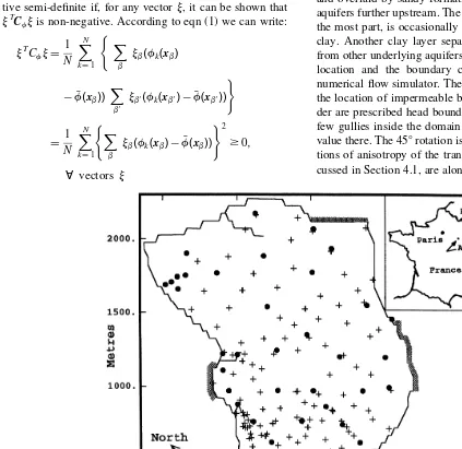
The case study is a sandy aquifer located in the north of France. While this aquifer represents part of the regional water table, hydrogeologically speaking, it can be treated as an individual entity. The principal sources of effective recharge are from rainfall where the aquifer is unconfined and overlaid by sandy formations, and from the adjoining aquifers further upstream. The aquifer, while unconfined for the most part, is occasionally confined above by a layer of clay. Another clay layer separates the aquifer in question from other underlying aquifers. Fig. 1 shows the aquifer, its location and the boundary conditions as input into the numerical flow simulator. The shaded grey zones represent the location of impermeable boundaries, while the remain-der are prescribed head boundaries. Also, the presence of a few gullies inside the domain imposes the maximum head value there. The 458rotation is made so that the main direc-tions of anisotropy of the transmissivity variogram, as dis-cussed in Section 4.1, are along the horizontal and vertical.
The simulation grid and finite differences grid are aligned to the new axes after this rotation.
It is the flexibility of the methodology based on joint flow simulations, as opposed to analytical models, that allows these complex physical features of the aquifer to be taken into account. The irregular boundary conditions, the effec-tive recharge, and the impermeability of overlying geologi-cal layers are all used as supplementary information by the numerical flow simulator during the calculation of each hydraulic head field. The subject of numerous geological and hydrogeological studies, this aquifer has been very well sampled. The position of the 41 transmissivity values and the 153 hydraulic head measurements is also shown in Fig. 1. The transmissivity ranges from 23 10¹6to 1.33 10¹3
m2/s with an average value of 2.1310¹4
m2/s.
4.1 Variographic analysis of the log-transmissivity
The variographic analysis of the transmissivity needs to take two factors into account: the error component associated with each experimental transmissivity value and the regu-larized nature of this data, that is, the fact that they do not represent punctual (i.e. point-support) values. Each trans-missivity value is representative of the area around the well over which the influence of the pumping test is felt by a modification to the pre-pumping aquifer level. This area, defined by the so-calledradius of action of the well, i.e. the distance from the well beyond which the drawdown caused by the pumping test is negligible, is the support over which the transmissivity measurement has been taken.
Under certain simplifying hypotheses23 the radius of action can be approximated as Ra¼1:5
Tt=S
p
where t is the pumping time andSthe storage coefficient. Each trans-missivity measurement is therefore assumed to be represen-tative of the average transmissivity within the circle of radiusRacentred on the well.
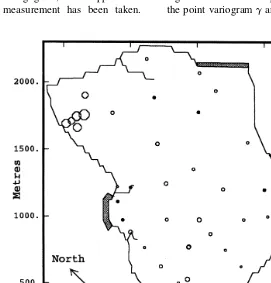
The distribution of the experimental Ra is presented in
Fig. 2, where the size of each open circle is proportional to the value ofRa. The lack of an accompanying piezometer
prevents us from calculating the radius of action for the five wells marked by a dot. Two distinct populations can be identified: the group of wells to the northwest of the aquifer having an averageRaof about 120 m, and the rest for which
the averageRais about 20 m. The first group is due to the
presence of recent superficial alluvial deposits only found in that part of the aquifer. To account for these differing sup-port sizes, the transmissivity data is divided into two groups, with the meanRaof each group being assigned to all wells
within that group as the support size associated with the transmissivity values.
Two series of experimental variograms are calculated. The first series is calculated from only the southern population (34 data), for which the average circular support has a radius of about 20 m. The second series is then calculated from all the data. In this case the average support size more than doubles. The regularization of a point variogram model allows us to correctly model the changing behaviour of the experimental variogram accord-ing to the size of the support considered. The link between the point variogramgand its regularized counterpartgRis
given by:
gR(h)¼measurement error variance
þ 1
VRaVRap
Z
VRa(x) du
Z
VRap(xþh)
g(u¹v)dv
whereVRa and VRap are the areas of the circular supports whose radii areRaandRa*, respectively. These circles are
centred on two points separated by the distance vectorh.
The measurement error variance, due to the incertitude associated with the transmissivity data, is discussed in the following paragraph. The sill and range of the point vario-gram model are chosen so that the resultinggR(h) correctly
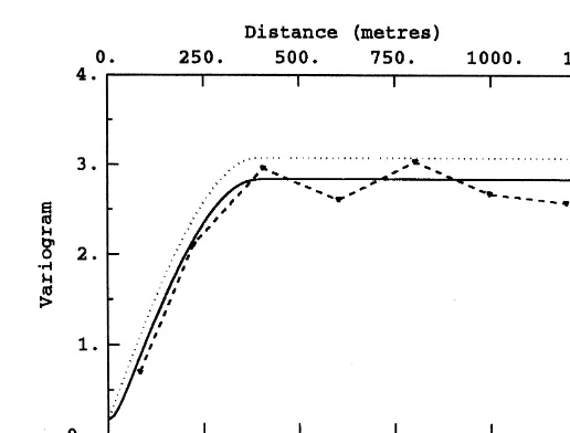
fits the experimental variograms for different support sizes. As an example Fig. 3 shows the omnidirectional variogram for all data fitted by a spherical variogram model: the con-tinuous line represents the regularized variogram model
gR(h) for which the support of the data is taken into
account, and the dotted line is its point support equivalent
g(h). Anisotropic behaviour was seen from the individual
directional variograms with the range of continuity in the northeast–southwest direction being about 2.5 times that seen in the northwest–southeast direction. As expected, the punctual model has both a higher sill and a less regular behaviour near the origin than its regularized counterpart. This punctual model, used to stochastically simulate the punctual transmissivity fields, produces a more variable and more locally erratic simulation than that which would have been obtained had a punctual model been directly fitted to the regularized data.
The apparent nugget effect in Fig. 3 has been fitted to take measurement errors of the data into account. Transmissivity values are calibrated from the experimental drawdown curve for each well test, so as to obtain the most satisfactory theoretical fit of the experimental curve. They therefore necessarily contain an error component that depends inversely on how well the experimental drawdown curve
represents the reality. Tests on the calibrated transmissivity values of the site24have shown that an overall factor of 5 defines a realistic confidence interval around the transmis-sivity data, i.e. the ratio between the highest and lowest plausible transmissivity values for a given well test. This multiplicative confidence interval is converted into an addi-tive one when dealing with the log-transmissivity. The resulting measurement error variance is calculated from standard normal confidence intervals and incorporated in the log-transmissivity variogram model as a discontinuity of 0.16 at the origin.
The log-transmissivity was simulated on a regular 535-m grid using the punctual variogram model presented in Fig. 3. Several upscaling techniques25have been proposed for well transmissivity data. Here we chose to obtain the simulated experimental data as the local equivalent transmissivity, the geometric mean, of the simulated points within the radius of action of each well. This radius varies between 11 and 180 m. So, between 13 and 970 punctual values are used to calculate the simulated values assigned to the data points.
4.2 Convergence of the log-transmissivity simulations
Before going on to the more complex step of cokriging with numerical covariances, kriging with numerical covariances should firstly be shown to be equivalent to kriging with the corresponding analytical covariance model. This equiva-lence depends on the convergence of the two-point statistics calculated over the series of log-transmissivity simulations, that can be tested from the evolution of the numerically obtained variance of lnT as a function of the number of simulationsN. From eqn (1), for a given pointx0:
Var(lnT(x0))N¼ 1
N
XN
k¼1
distribution of the numerical variance calculated for a given pointx0: Var(lnT(x0))N,(j2=N)x2N¹1, allows the
construc-tion of confidence intervals around j2, the theoretical variance of lnT. We consider 10 different points chosen at random in the field and calculate Var(lnT)Nfor each of
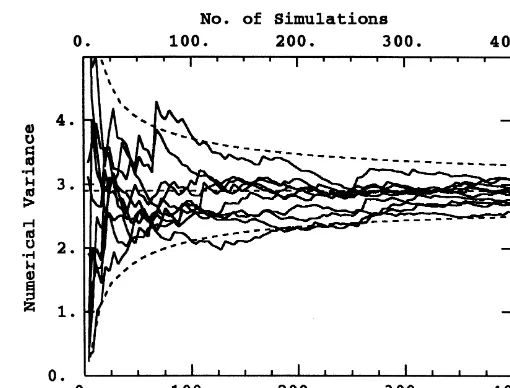
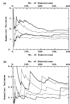
them. Fig. 4 presents the evolution of Var(lnT)Nas a
func-tion ofN, the underlying simulated variancej2¼2.9 and the 95% confidence interval (the dashed curves) around it. The width of this interval, i.e. the expected fluctuations of Var(lnT)N, decreases slowly so that even after 400
simula-tions the residual fluctuasimula-tions can represent up to 14% of the true variance. This slow convergence rate, that depends on 1/ÎN, implies that even by doubling the number of simulations (N¼800), fluctuations of up to 11% can still be expected.
We note here that the convergence of the numerical variance depends on the convergence of the numerical mean as seen by the form of eqn (4) in the case of the head variation. Any residual fluctuations in the numerical mean are necessarily carried by the numerical variance. So the convergence of the numerical variance implicitly implies the convergence of the corresponding mean. For this reason, behaviour of the numerical mean has not been considered here. These comments also apply to the head variation simulations discussed in the next section.
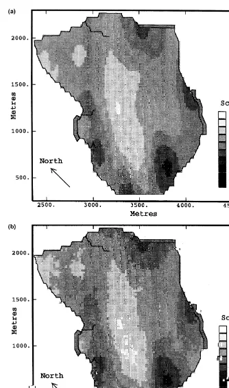
To visualise the effect of these residual fluctuations, lnT
is kriged with both the analytical covariances and the numerical covariances calculated from the 400 simulations (Fig. 5). It is reminded that, when considering the transmis-sivity data in units of 10¹6
m2/s, lnTranges between 0.79 and 7.18, with an average value of 4.37. While globally the two kriged maps present the same characteristics, locally the numerically kriged map displays fluctuations not seen when kriging with analytical covariances. These fluctuations, quantified as the standardised difference between the two maps for each point, were shown to be normally distributed with a zero mean and a standard deviation of about 8% over
the field. So, when compared with the analytically based method, the numerical kriging result is globally unbiased but presents local fluctuations that are the same order of magnitude as those displayed in the calculation of the numerical covariances themselves.
4.3 Convergence of the hydraulic head
The hydraulic head field corresponding to a simulated trans-missivity field is obtained via a slightly modified finite dif-ferences algorithm that produces a globally unbiased result. The dimensions of the finite differences grid mesh (20 3 50 m) are chosen to reflect the ratio of the longest and shortest ranges of continuity seen in the anisotropic log-transmissivity variogram. There are 40 punctual simulated transmissivity values within each grid mesh. The inter-face transmissivity, calculated as the geometric mean of the 20 simulated transmissivity values within a diamond-shaped support that extends from one mesh centre to the next, is directly entered into the numerical flow simulator26. The series of hydraulic head fields are obtained for a constant set of physical parameters (boundary conditions, effective recharge, etc.). The numerical head variation covariances are calculated after having subtracted the mean head from each head field. As for lnT, the conver-gence of the head variation is tested by the evolution of its numerically obtained variance as a function of the number of simulations. However, the distribution off(x0) depends on the location of the point x0 considered11. The head variation is highly skewed with a low variance near the prescribed head boundaries but has a symmetrical distri-bution and a high variance over the central part of the aquifer.
because its variance is not constant over the field, it is not possible to associate confidence intervals to these results. The behaviour for the symmetrically distributed central points is similar to that of the normally distributed lnT. On the other hand, for those points near a prescribed head boundary, being highly sensitive to the occasional large
value, the evolution of the numerical variance presents some very important jumps even towards the end of the 400 simulations. This means that more simulations would be needed to dramatically reduce the fluctuations in the f
numerical covariances when there are experimental data points near a prescribed head boundary.
4.4 Transmissivity estimation
Given the relatively important residual fluctuations seen in the numerically calculated variance off, it is to be expected that the corresponding cokriged transmissivity estimation will also present some artificially introduced local variabil-ity. On the numerically cokriged log-transmissivity field (Fig. 7), this local variability is especially noticeable in the zone around the western impermeable boundary where the estimated lnT takes on a very spotty appearance. This may be due to the influence of some neighbouring head variation data that are close to a prescribed head boundary. The striking feature of the cokriged result is the increased variability of the lnT estimate when compared with the kriged result (Fig. 6). The kriging weights for our case study were always seen to be between 0 and 1. In this case the resulting kriging estimator, a linear interpolator of the lnT data, is limited in value by the range of the experimental data themselves. The cokriging estimator, on the other hand, takes both the lnTandfdata into account
with the weight assigned to the second variable being deter-mined by the cross correlations which can be either positive or negative, according to the relative position of the points considered8. There is therefore no obvious a priori limit to the range of values, i.e. the variability, of the cokriging estimate. This can be seen in the southern part of the aquifer where the kriged estimate is replaced by a much lower cokriging estimate. This is especially pleasing as this low cokriged transmissivity agrees with hydrogeological studies of the aquifer that confirm the existence of important head gradients in this part of the aquifer that can only come from very low transmissivity values. Similarly, the zone of high cokriged transmissivity seen through the central part and to the north corresponds well with the manual calibration of the aquifer in a zone that is known to have a smooth head profile. So, the cokriged map presents features that, coming from the influence of the head data and therefore unseen on the kriged map, are consistent with the hydrogeologist’s manual interpretation of the aquifer’s characteristics.
It must be stressed, however, that the cokriged map does Fig. 6.(a) Evolution of the numerically calculatedfvariance for five central points. (b) Evolution of the numerically calculatedfvariance
not reproduce the reality. It can only be used as an indicator of the global behaviour in the transmissivity representing the most likely value of the transmissivity at any point, given the neighbouring transmissivity and head values. In particular the linear cokriging estimate only respects the degree of linear relationship between the two variables, and not the non-linear relationship given by the flow equa-tion. The solution of the flow equation in the cokriged trans-missivity field will not produce heads equal to the measured head values. Should one be interested in the correct repro-duction of the head field from the resulting transmissivity field, simulations should be considered.
5 CONCLUSION
The combination of geostatistics and numerical flow simu-lators thus provides a powerful technique for reconstructing the transmissivity field from the available transmissivity and head data. Using a probabilistic framework to model the spatial behaviour of the transmissivity, the corresponding hydraulic head field is determined by a numerical flow model based on a modified finite differences algorithm. A series of such joint flow simulations leads to the numerical calculation of the direct and cross covariances needed to cokrige the transmissivity. The cokriging estimator is pre-ferred to the kriging estimator so as to incorporate the influ-ence of the more numerous and more precise hydraulic head data in the estimated transmissivity field. For the practical application presented here, it was shown that a large number of joint flow simulations is necessary for the numerically
calculated covariances to converge. This is the sole dis-advantage of the numerical method when compared with available first-order analytic methods: it is computer intensive with respect to the number of simulations required and the space required to store the necessary numerical covariances.
On the other hand, the proposed method is very flexible. The standard first-order approximations, multi-Gaussian assumptions and constraints on boundary conditions or the effective recharge of analytical approaches are no longer needed when solving the diffusion equation with a numer-ical flow simulator, and could not realistnumer-ically be applied to the case study treated. So, for those cases where the use of quicker analytical techniques is not possible, the proposed numerical method provides a solution that is consistent with the physical relationships that govern groundwater flow.
ACKNOWLEDGEMENTS
This work was financed by the BRGM. The authors would also like to thank the French Government Agency ANDRA for the use of the data, and P. Delfiner, J.P. Del-homme, G. de Marsily and G. Matheron for their comments. Thanks also go to the reviewers for their remarks that have improved the presentation of this paper.
REFERENCES
1. RamaRao, B.S., LaVenue, A.M., de Marsily, G. and Mar-ietta, M.G. Pilot point methodology for automated
calibration of an ensemble of conditionally simulated trans-missivity fields, 1. Theory and computational experiments.
Water Resources Research, 1995,31(3), 475–494.
2. Gomez-Hernandez, J.J., Capilla, J.E. and Sahuquillo, A., Inverse conditional simulations. InGeostatistics Wollongong ’96, ed. E.Y. Baafi and N.A. Shofield. Kluwer, Dordrecht, Netherlands, Vol. 1, 1997, 282–291.
3. LaVenue, A.M., RamaRao, B.S., de Marsily, G. and Mar-ietta, M.G. Pilot point methodology for automated calibration of an ensemble of conditionally simulated transmissivity fields, 2. Application. Water Resources Research, 1995,
31(3), 495–516.
4. Ginn, T.R. and Cushman, J.H. Inverse methods for subsur-face flow: A critical review of stochastic techniques. Stochas-tic Hydrol. Hydraul., 1990,4,1–26.
5. Mizell, S.A., Stochastic analysis of spatial variability in two-dimensional steady groundwater flow with implications for observation-well network design. Doctorate thesis, New Mexico Institute of Mining and Technology, Socorro, NM, 1980.
6. Hoeksema, R.J. and Kitanidis, P.K. An application of the geostatistical approach to the inverse problem in two-dimensional groundwater hydrology modelling. Water Resources Research, 1984,20(7), 1003–1020.
7. Kitanidis, P.K. and Vomvoris, E.G. A geostatistical approach to the inverse problem in groundwater hydrology modelling (steady state) and one dimensional simulations. Water Resources Research, 1983,19(3), 677–690.
8. Dong, A., Estimation ge´ostatistique des phe´nome`nes re´gis par des e´quations aux derive´es partielles. Doctorate thesis, Ecole des Mines de Paris, Fontainebleau, France, 1990, 211 pp.
9. Hoeksema, R.J. and Kitanidis, P.K. Comparison of con-ditional mean and kriging estimation in the geostatistical solution to the inverse problem.Water Resources Research, 1985,21(6), 825–836.
10. Rubin, Y. and Dagan, G. Stochastic identification of trans-missivity and effective recharge in steady state groundwater flow: 1. Theory and 2. Case study. Water Resources Research, 1987,23(7), 1185–1200.
11. Roth, C., Contribution de la ge´ostatistique a` la re´solution du proble´me inverse en hydroge´ologie. Doctorate thesis, Ecole des Mines de Paris, Editions BRGM, Orle´ans, France, 1995, 196 pp.
12. Dagan, G. Stochastic modelling of groundwater by uncon-ditional and conuncon-ditional probabilities: the inverse problem.
Water Resources Research, 1985,21(1), 65–72.
13. Gehlar, L.W., Stochastic Subsurface Hydrology. Prentice-Hall, Engelwood, New Jersey, 1993.
14. Certes, C. and de Marsily, G., Application of the pilot point
method to the identification of aquifer transmissivities.
Advances in Water Resources, 1991,14(5).
15. Sahuquillo, A., Capilla, J., Gomez-Hernandez, J.J. and Andreu, J., Conditional simulation of transmissivity fields honouring piezometric data. In Fluid Flow Modelling, ed. W.R. Black and E. Cabrera. Computational Mechanics Pub-lications, 1992, pp. 201–212.
16. Hoeksema, R.J. and Clapp, R.B., Calibration of groundwater flow models using Monte Carlo simulations and geostatistics. In Proceedings of the ModelCARE 90 Conference, The Hague, September 1990, IAHS Publ. No. 195, 1990, pp. 33–42.
17. Alfaro Sironvalle, M., Etude de la robustesse des simulations de fonctions ale´atoires. Doctorate thesis, Ecole des Mines de Paris, Fontainebleau, France, 1979.
18. Chile`s, J.P. and Delfiner, P., Using FFT techniques for simu-lating gaussian random fields. InProceedings of the Confer-ence on Mining Geostatistics, Kruger National Park, South Africa, 19–22 Sept. 1994. Geostatistical Association of South Africa, Johannesburg, 1996, pp. 131–140.
19. Prickett, T.A. and Lonnquist, C.G. Selected digital computer techniques for groundwater resource evaluation.Illinois State Water Survey Bulletin, 1971,55,1–62.
20. Romeu, R.K. and Noetinger, B. Calculation of internodal transmissibilities in finite difference models of flow in heterogeneous media. Water Resources Research, 1995,
31(4), 943–959.
21. Roth, C., de Fouquet, C., Chile`s, J.P. and Matheron, G., Geostatistics applied to hydrogeology’s inverse problem: taking boundary conditions into account. In Geostatistics Wollongong ’96, ed. E.Y. Baafi and N.A. Shofield. Kluwer, Dordrecht, Netherlands, Vol. 2, 1997, 1085–1097.
22. Matheron, G., The theory of regionalised variables and its application, Fascicule 5. Cahiers du Centre de Morphologie Mathematique, Fontainebleau, France, 1971, 211 pp. 23. de Marsily, G., Quantitative Hydrology: Groundwater
Hydrology for Engineers. Academic Press, San Diego, CA, 1986, 440 pp.
24. Lavie, J., Site de stockage de l’Aube: Soulaines-Dhuys (Aube). Mode´lisation en re´gime transitoire de la nappe des sables aptiens du pli de Soulaines a` l’e´tat naturel, BRGM Report No. 88 SGN 776 STO, BRGM, Orle´ans, France, 1988.
25. Desbarats, A.J. Geostatistical analysis of interwell transmis-sivity in heterogeneous aquifers.Water Resources Research, 1993,29(4), 1239–1246.