CRUCIAL POINTS OF INTERFEROMETRIC PROCESSING
FOR DEM GENERATION USING HIGH RESOLUTION SAR DATA
Sefercik, U. G.*, Dana, I.**
* Zonguldak Karaelmas University, Turkey
[email protected]
** Romanian Space Agency, Romania
[email protected]
KEY WORDS: InSAR, DEM, Generation, TerraSAR-X, Comparison
ABSTRACT:
Data collection for digital elevation model (DEM) generation can be carried out by two main methods in space-borne remote sensing such as stereoscopy using optical or radar satellite imagery (stereophotogrammetry, respectively radargrammetry) and interferometry based on interferometric synthetic aperture radar (InSAR) data. These techniques have advantages and disadvantages in comparison against each other. Especially filling the gaps which arise from the problem of cloud coverage in DEM generation by optical imagery, InSAR became operational in recent years and DEMs became the most demanded interferometric products. Essentially, in comparison, DEM generation from synthetic aperture radar (SAR) images is not a simple manner like generation from optical satellite imagery. Interferometric processing has several complicated steps for the production of a DEM. The quality of the data set and used software package come into prominence for the stability of the generated DEM.
In the paper, the interferometric processing steps for DEM generation from InSAR data and the crucial threshold values are tried to be explained. For DEM generation, a part of Istanbul (historical peninsula and near surroundings) was selected as the test field because of data availability. The data sets of two different imaging modes (StripMap ~ 3 m resolution and High Resolution Spotlight ~ 1 m resolution) of TerraSAR-X have been used. At the implementation, besides the determination of crucial points at interferometric processing steps, to define the effect of computer software, DEM production have been performed using two different software packages in parallel and the products have been compared In the result section of the paper, besides the colorful visualizations of final products along with the height scales, accuracy evaluations have been performed for both DEMs with the help of a more accurate reference digital terrain model (DTM). This reference model has been achieved by large scale aerial photos. Normally, it has a 5 m original grid spacing, however it has been resampled at a spacing of 1 m towards the needs of the research.
1. INTRODUCTION
A Digital Elevation Model (DEM) is the digital cartographic representation of the elevation of the terrain at regularly spaced intervals in X and Y directions, using Z-values related to a common vertical datum. DEMs are required for several purposes and applications, by different working groups from various disciplines. In order to satisfy the demand, various DEM generation techniques have been developed up to now. Remote sensing is one of those techniques and contains two main methods for DEM generation: optical and radar satellite imagery and interferometry (InSAR).
InSAR is a technique to derive DEM from at least two complex SAR images. The data are either taken simultaneously (single-pass mode) or sequentially (repeat-(single-pass mode) by airborne or space-borne sensors from slightly different points of view on the same interest area (Crosetto and Perez Aragues, 1999). A general review of the technique is given in Rosen et al. (2000) and Richards (2007). Repeat-pass interferometry is affected by temporal de-correlation and errors in baseline determination (Massonnet and Souyris, 2008). One of the most advanced repeat-pass systems is the German TerraSAR-X (TSX) satellite which has been launched on June 15th
, 2007. TSX offers very high resolution (~1 m in the High Resolution Spotlight mode) imagery, which could not be achieved from radar technologies. The spatial resolution and the information content of the TSX images are similar to high resolution optical imagery. In
contrast to optical sensors, TSX can be operated under all weather conditions without being influenced by clouds.
Utilizing the advantages of InSAR technique, indeed the planimetric and altimetric locations of target ground objects can be determined. Based on complex InSAR data interferograms (fringe maps) can be generated and applying interferometric processing steps DEMs can be created up to global coverage. However, in this case, the processing chain is not an easy procedure and has several steps to reach the DEM. This situation represents the structure of the present study and also the main processing phases, critical thresholds and encountered challenges will be explained.
2. TEST FIELD
As known, Istanbul (Turkey) is one of the biggest cities in the world. About 14 million people leave in the city and most of settlements are at the surrounding of Bosporus and coast line of Marmara Sea. The test area of the study is a part of Istanbul and covers 10 km × 8 km. It includes the historical peninsula and near surroundings. Historical Peninsula (Old City) is one of the most important regions in Istanbul because of its historic heritage, located on the European side, neighbored to the Bosporus and Marmara Sea. Figure 1 shows the test field with the frequency distribution of terrain inclination. The elevation reaches from sea level up to 130 m.
Figure 1. Test field and frequency distribution of terrain inclination
3. SAR DATA SETS
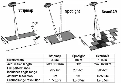
TSX is built in Germany and its lifetime will be at least 5 years. The satellite uses 3 different operation modes as StripMap (SM), Spotlight - includes Spotlight (SL) and high resolution Spotlight (HS) modes with sequentially 2m and 1m resolution - and ScanSAR. These modes provide high resolution images for detailed analysis as well as wide swath data whenever a larger coverage is required. The imaging can be possible in single, dual and quad-polarization. TSX has single look complex data type and uses repeat-pass interferometry for the DEM generation by interferometry (URL-1). Figure 2 shows the geometries of imaging modes and their characteristics.
Figure 2. The TerraSAR-X geometries of imaging modes and their characteristics (Eineder et al. 2003)
In this research, two different operation modes of TSX (SM and HS) and two corresponding SAR image-pairs (four SAR images
have been used for the DEM generation. When operating in StripMap mode, TSX acquires long strips up to 1650 km length with 30 km swath width. The ground swath is illuminated with a continuous sequence of pulses while the antenna beam is fixed in elevation and azimuth. This results in an image strip with continuous image quality in azimuth (Roth, 2003). In Spotlight mode, during the observation of a particular ground scene the radar beam is steered like a spotlight so that the area of interest is illuminated longer and hence the synthetic aperture becomes larger. The maximum azimuth steering angle range is ± 0.75º (Roth, 2003). The image-pairs of TSX SM and HS and their characteristics can be seen at the following figures 3, 4 and tables 1, 2.
Figure 3. TSX SM Istanbul SAR image-pair
Figure 4. TSX HS Istanbul SAR image-pair
Table 1. Characteristics of TSX SM Istanbul SAR image-pair Characteristics TSX SM Image 1 TSX SM Image 2
Beam strip_012 strip_012
Start date 2008-02-11T04:10:31,531
2008-03-15T04:10:31,957 End date
2008-02-11T04:10:38,077
2008-03-15T04:10:38,504 Polarization
mode/Channel Single/HH Single/HH
Looking/Pass direction
Right looking Descending pass
Right looking Descending pass International Archives of the Photogrammetry, Remote Sensing and Spatial Information Sciences, Volume XXXVIII-4/W19, 2011
Table 2. Characteristics of high resolution TSX SL Istanbul
mode/Channel Single/HH Single/HH Looking/Pass
4. INTERFEROMETRIC PROCESSING STEPS
Interferometric processing steps of DEM generation are not as simple as DEM generation with optical imagery. The operator has to apply several complex steps and assign threshold values depending on the quality and characteristics of the SAR data For DEM generation from SAR data, SARscape module of ENVI version 4.6 and the InSAR module of ERDAS Imagine version 9.3 were used. ENVI SARscape is a powerful module that allows processing of SAR data using several sub-modules. Also, ERDAS InSAR follows a very well structured interferometric processing chain. In principle, the under-mentioned processing steps are followed for the interferometric processing by both InSAR processing softwares:
9 Baseline estimation and co-registration 9 Interferogram generation and flattening 9 Coherence and interferogram filtering 9 Phase unwrapping
9 Orbital refinement
9 Phase to height conversion and geocoding
When starting the interferometric processing, firstly two InSAR images are imported by definition of data formats, sensors, data types and reference extensible markup language (xml) parameter files and the processing steps mentioned above were applied sequentially up to DEM generation.
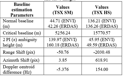
Baseline estimation and co-registration
The baseline estimation and co-registration are of vital importance for interferometric processing. To apply these two steps, one reference SAR image titled as master and one second image which has similar acquisition geometry named as slave ought to be available. The master and slave images should overlap to achieve sub-pixel accuracy in the slant range geometry. The baseline estimation includes relevant parameters shown in Table 3. The normal baseline is the perpendicular baseline between the master and slave orbit which is important for further interferometric processing. In principle, a higher normal baseline is equivalent with a higher accuracy in DEM generation. But, if the magnitude of normal baseline exceeds the threshold values, the noise that affects the interferogram increases and the description of the topography and DEM generation become complicated. The critical normal baseline is given by the acquisition geometry and by the characteristics of the SAR sensor. An optimal value for the normal baseline maximizes the signal-to-noise ratio (Gatelli et al., 1994), (Bamler, 1997), (Bamler, 2006), (Ferretti et al., 2007). Hence, the critical baseline should not be exceeded in any case. The 2 π ambiguity height represents the height difference concerned
with an interferometric fringe (2 π cycle). The increase of this value obstructs the definition and delineation of small height changes. The range and azimuth shifts will be applied in range and azimuth direction during the master-slave coarse co-registration. The difference between master and slave Doppler centroids is named as Doppler centroid difference (fD). This
value equals to 0 (zero) when the side look is 90º during the satellite travels on its flight direction (azimuth). Apart from that situation fD continually has a value different from 0 and which
cannot exceed the pulse repetition frequency (critical value).
In this research, TSX SM image 1 was selected as master and TSX SM image 2 as slave. In the same manner TSX HS image 1 was selected as master and TSX HS image 2 as slave. The baseline estimation results of TSX SM and TSX HS image-pairs are shown in Table 3.
Table 3. Baseline estimation between TSX SM and HS master and slave images Critical baseline (m) 5256.24 15770.57 2 PI (π) ambiguity
difference (Hz) -5.376 154.00
The co-registration of complex SAR images is extremely important for interferogram generation. This interferometric processing step is accomplished in two steps (Rabus et al., 2003), (Li and Bethel, 2008): coarse co-registration (with an accuracy of 1-2 pixels) and fine co-registration (with an accuracy of 1/10 pixel). At first, the location of each pixel in the slave image changes with respect to the master. Then amplitude and phase information of slave image is recalculated for each pixel by interpolation (Gens, 1998), using bilinear or cubic convolution functions. The slave image resampling method is chosen upon the type of terrain and the quality of the complex SAR images. At the co-registration, dependencies, range and azimuth grid positions and window numbers, initialization from orbit, orbit accuracy and orbit interpolation values have to be calibrated. Additionally, the window sizes, central positions of range and azimuth and cross correlation threshold value should be assigned. Eventually, fine shift parameters should be determined as well as containing window sizes, range and azimuth window numbers, cross correlation oversampling value, coherence oversampling value, reject and signal to noise ratio (SNR) threshold values. The number of tie points (grid density), the width of the search window and the threshold for the correlation coefficient are extremely important in this step as they influence the final results (DEM accuracy) of the interferometric processing. These values are usually determined by repeated tests.
Interferogram Generationand Flattening
In this research, besides master and slave images, DEMs derived from SPOT-5 HRS and SRTM (3 arc seconds spatial resolution ~ 71 m at the latitude of the test area) and the precise International Archives of the Photogrammetry, Remote Sensing and Spatial Information Sciences, Volume XXXVIII-4/W19, 2011
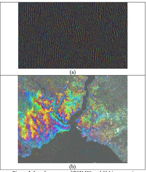
orbital parameters were used for the interferogram generation. The use of a DEM (optional process) for interferogram generation allows the assignment of a reference cartographic system for the resulting DEM. In case of SAR images acquired at large periods of time, temporal de-correlation affects the quality of the interferometric phase and this phenomenon is translated into noise. Noise reduction is performed by averaging the neighboring pixels of the complex interferogram with the cost of lowering its spatial resolution. This process is called interferogram multilooking (Ferretti et al., 2007), (Manjunath, 2008). The multilooking factor is computed based on the slant range and azimuth resolution and on the incidence angle at the center of the scene. The generated interferograms from TSX HS SAR image-pair and TSX SM SAR image-pair can be seen in Figure 5 (a and b).
After interferogram generation, several low frequent components can be removed using interferogram flattening which is the differential phase between the constant phase and the phase expected for a flat or a known topography. Therefore, this step consists of the removal of the interferometric phase component due to terrain topography. This is not a main step at interferometric processing, it is used just to support the phase unwrapping process. At the end of interferogram flattening, the numbers of fringes are reduced.
(a)
(b)
Figure 5. Interferograms of TSX HS and SM image-pair
Coherence and Interferogram Filtering
The interferometric coherence represents the stability of the backscattered SAR signal over an area of interest (Parcharidis et al. 2005). It can be summarized as a ratio between coherent and incoherent synopsis. The coherence ranges between 0 (the phase is just noise) and 1 (complete absence of noise) depending upon the noise of the SAR sensor, errors that occurred during the previous interferometric steps (low accuracy co-registration), acquisition geometry (looking direction and incidence angle), systematic spatial de-correlation
(due to terrain topography, slope, height differences), and temporal de-correlation between master and slave image (Gatelli et al., 1994), (Zhou et al., 2009). The large acquisition interval conducted to the significant decrease of the coherence.
Figure 6.a. Filtered interferogram and coherence map – TSX HS images
Figure 6.b. Filtered interferogram and coherence map – TSX SM images
Coherence maps are achieved via measuring pixel-to-pixel signal to noise ratio (SNR) and they expose the quality and reliability of an interferogram. For the generation of a coherence map, an interferogram or its filtered version can be used. The use of a filtered interferogram may be useful for higher coherence. Filters do not necessarily enhance or recover the radar signal but a powerful filter reduces noise, caused by temporal or baseline related de-correlation, changes the structure of the interferogram and improves fringe visibility. In this research, Goldstein, one of the powerful adaptive radar interferogram filters which was developed by R. M. Goldstein and C. L. Werner has been used. Figure 6 (a and b) shows the filtered interferograms of TSX HS and TSX SM (upper side) and their corresponding coherence maps (lower side). The bright parts of the coherence map indicate areas with higher coherence like flat areas and the dark parts indicate regions with lower coherence like sea, forest etc.
Phase Unwrapping
Phase unwrapping is the most complex step of interferometric processing and problems occur from aliasing errors due to phase noise by low coherence and under sampling phenomena because of locally high fringe rates (Reigber and Moreira 1997). For the solution of this problems several algorithms like region growing, minimum cost flow, minimum least squares, etc. have been developed. A thorough description of different phase unwrapping algorithms can be found in Ghiglia and Pritt (1998) and (Richards, 2007). In this research, for phase unwrapping two different approaches have been applied: region growing algorithm (see Reigber and Moreira 1997) was used with different decomposition levels and minimum cost flow algorithm (Ferretti et al., 2007). The region-growing method can be described in terms of two primitive operations: the translate operation, which adds/subtracts 2π to all points of a region, and the connect operation, which merges two areas. Starting from a condition of maximum fragmentation -each point constitutes a region - these two operations are executed iteratively on the active areas until no more joins can be done (Baldi 2003). The minimum cost flow (MCF) algorithm assumes that the wrapped phase field is independent of the path followed for the integration of the phase discontinuities (caused by terrain topography, acquisition geometry, interferometric phase noise, and normal baseline). In this way, the MCF algorithm minimizes the number of full cycles. This phase unwrapping algorithm offers very good results for areas with moderate terrain, whereas for mountainous areas the editing of the resulting DEM is necessary (Rabus et al., 2003). The resulting interferogram (by region growing algorithm) of TSX HS images after the phase unwrapping step can be observed in Figure 7.
Figure 7. Interferogram of TSX HS images after phase unwrapping
Orbital Refinement
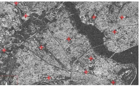
In fact, the relation between the phase difference and the elevation is a function of the baseline and an accurate baseline is demanded for an accurate DEM. The baseline is initially estimated using the orbit information of the image header file and the orbital refinement improves the accuracy of the baseline value. In this process, besides the refining of orbits, phase compensation is calculated using ground control points (GCPs), therefore it enables the absolute phase calculation. The GCPs should be located on flat and highly correlated areas (coherence map can be used for this process). According to the 7 parameters transformation, at least 7 GCPs are required, but at least 10-12 GCPs should be used for a satisfying over determination. In this research, 12 GCPs were used for the orbital refinement of TSX SM and TSX HS interferograms. Figure 8 shows the GCP distribution on TSX HS coherence map.
Figure 8. GCPs distribution on TSX HS interferogram and coherence map
As result of this processing step, no new output file is generated because this is just a modification of the existing phase unwrapping header file (.sml) and this file is re-registered in itself.
Phase to Height Conversion and Geocoding
At the last step of interferometric processing for DEM generation, phase values should be converted to the height for each pixel of the interferogram. The conversion implies the re-projection from the SAR coordinate system of the complex images into a geocentric Cartesian system defined by X, Y planimetric coordinates and Z height (Crosetto and Perez Aragues, 1999), (Ferretti et al., 2007). The final result of this step is represented by a DEM. Geocoding process of SAR images is different from optical imagery. SAR systems cause a non-linear compression that’s why they cannot be corrected using polynomials. The sensor and processor characteristics have to be considered at the geometric correction.
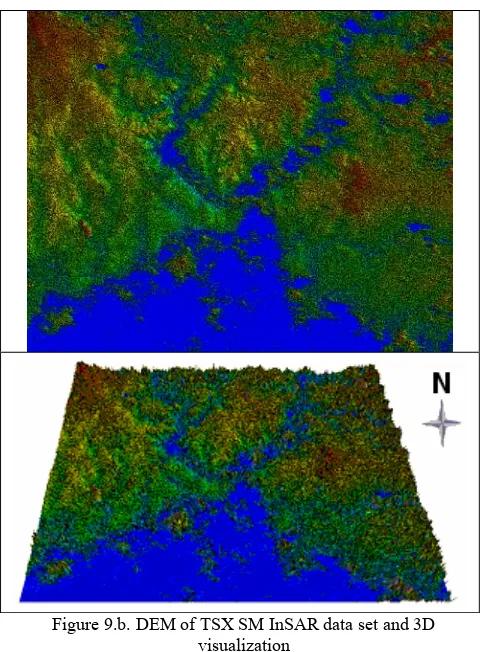
For phase to height conversion and geocoding some critical values should be determined like coherence threshold, interpolation method, interpolation window size, mean window size and requested grid size. Figure 9 shows the DEM derived by TSX SM (10 m grid spacing) and its 3D visualization using an exaggeration factor of 10 (a) and 5 (b). Figure 10 shows the DEM derived by TSX HS (3 m grid spacing) and its 3D visualization using an exaggeration factor 5.
Figure 9.a. DEM of TSX SM InSAR data set and 3D visualization (10 m grid spacing, 10 – Z exaggeration factor)
Figure 9.b. DEM of TSX SM InSAR data set and 3D visualization
(10 m grid spacing, 5 – Z exaggeration factor)
Figure 10. DEM of TSX HS InSAR data set and 3D visualization (3 m grid spacing)
5. EVALUATION OF DEMs
The planimetric and altimetric accuracy of a DEM generated by means of interferometry is affected by the following factors: the accuracy of the interferometric phase computation, the accuracy of the geometry acquisition determination and the accuracy of the atmospheric errors removal. More over, the accuracy is depending upon the phase unwrapping results (Bamler, 1997), (Kyaruzi, 2005), (Ferretti et al., 2007), (Richards, 2007), (Mohr and Merryman Boncori, 2007). From the theoretical point of view, the InSAR technique is assumed to generate DEMs with an accuracy in the order of a few meters (Coulson, 1993) depending upon the quality of SAR data sets. Thus, the quality may be expected especially from TSX HS mode.
The accuracy of a DEM can be assessed by various procedures. One of the most common procedures, for example, is the comparison with a reference DEM (Lin et al.1994). This is one of the powerful ways to understand the quality of a DEM and it has been applied in this research. The most critical point on this method is that the reference DEM has to be more accurate than the evaluated DEM and has no distortion on the comparison area. For this research, a more accurate (10 cm- 1 m) DTM, derived by 1:1000 scale aerial photos was used as reference for the evaluation process. This reference covers the test area and has 1 m grid spacing. The evaluated DEMs are reduced into the limits of the reference and a group of refinement processes (shifts, manipulations, blunder filtering, gap filling etc.) have been carried out before the accuracy assessment. The results of the accuracy analysis are presented in Table 4. For the accuracy analysis, a DEM evaluation system BLUH (Bundle Block Adjustment Leibniz University Hannover) has been used, developed by Dr. Karsten Jacobsen from Leibniz University International Archives of the Photogrammetry, Remote Sensing and Spatial Information Sciences, Volume XXXVIII-4/W19, 2011
Hannover, Institute of Photogrammetry and GeoInformation. The results of accuracy analysis can be seen at Table 4.
Table 4. Accuracy assessment of DEMs
(SZ= Standard deviation of Z differences in comparison with reference DEM, α= slope)
In this investigation, the interferometric processing procedure for digital elevation model generation has been described, using two different acquisition modes SAR image-pairs of the current satellite TerraSAR-X, in Istanbul test field, Turkey. These different acquisition modes are StripMap (3 m) and the High Resolution Spotlight (1 m) image-pairs with respectively ~45 m and ~135 m normal baselines.
It can be observed that in contrast to optical imagery, DEM generation by SAR data has several complicated steps and during the interferometric processing chain many critical threshold values have to be applied.
The spatial resolution plays a significant role in the generation of height models by InSAR because of the intensity of collected data. The spatial resolution and the information content of the TerraSAR-X images are similar to the high resolution optical images.
The co-registration of the SAR images plays a very important role in all the following interferometric processing steps. The width of the search window, the number of tie points and the correlation threshold represent critical parameters in this stage. These parameters are usually set based on a number of experimental tests.
The multilooking factor that is used for interferogram generation has also a great impact on the final results. This parameter has to be fine tuned in order to produce the maximum noise reduction, but, at the same time to keep a superior spatial resolution.
The synthetic interferogram computed using an accurate DEM (with satisfying spatial resolution) improves the results. Thus, the removal of the phase component due to the topography of the terrain is performed more precisely.
The differential interferogram is characterized by the height of ambiguity. A lower value for the height of ambiguity means a more sensitive SAR signal to height differences.
Coherence map has a significant role at the interferometric processing. The visualization of the stability and interior integrity of a filtered interferogram and coherence threshold is one of the most critical choices to eliminate the low coherence
details without loosing many of them. The filtering of the interferogram is recommended.
Phase unwrapping is the most complex step of interferometric processing and several algorithms have been improved for the solution of it. The results of the phase unwrapping step mainly depend on the algorithm used and on the coherence threshold values. A lower value means that more points will be used for DEM generation, but with less phase accuracy. Similar, a higher value will assume less points, but with superior phase accuracy.
Orbital refinement is recommended. The accuracy of the resulting DEM is clearly improved when using the corrected normal baseline. It is emphasized that in comparison with stereo-optical imagery, the number of GCPs and the distribution logic is totally different and it is not mandatory to measure GCPs on the ground. Coherence map comes into prominence to determine the coherent regions for GCP selection.
The normal baseline of the SAR-image-pair is one of the most important factors for TerraSAR-X digital elevation models. A too short baseline is not leading to the required details and it is not enough to accurately estimate the terrain topography. The digital surface model of TerraSAR-X High Resolution Spotlight based on a longer baseline is 30% more accurate as the TerraSAR-X StripMap digital surface model.
ACKNOWLEDGEMENTS
Thanks are going to Turkish Scientific and Technical Research Institute (TÜBİTAK), Turkey, Romanian Space Agency, Romania, and DLR, Germany, for their supports to this research. The TerraSAR-X images were acquired in the framework of the general proposal "Evaluation of DEM derived from TerraSAR-X data" (ID LAN_0634), submitted to DLR in 2009. And also we would like to thank Prof. Dr. Uwe Sörgel and Dr. Karsten Jacobsen from Leibniz University Hannover, Institute of Photogrammetry and GeoInformation.
REFERENCES
Baldi, A., 2003. Phase Unwrapping by Region Growing, Applied Optics, Vol. 42, Issue 14, pp. 2498-2505
Bamler, R., 1997. Digital Terrain Models from Radar Interferometry, Photogrammetric Week, Stuttgart, Germany
Bamler, R., 2006. Radar Interferometry for Surface
Deformation Assessment, Summer School Alpbach 2006:
Monitoring of Natural Hazards from Space, Alpbach, Austria
Coulson, S.N., 1993. SAR interferometry with ERS-1, Earth Observation Quarterly, no: 40, pp. 20-23
Crosetto, M., Perez Aragues, F., 1999. Radargrammetry and SAR Interferometry for DEM Generation: Validation and Data
Fusion, Proceedings of SAR Workshop: CEOS Committee on
Earth Observation Satellites, ISBN: 9290926414, Toulouse, France
Eineder, M., Runge, H., Boerner, E., Bamler, R., Adam, N., Schättler, B., Breit, H. and Suchandt, S., 2003. SAR Interferometry with TerraSAR-X, Proceedings of the FRINGE 2003 Workshop (ESA SP-550), 1-5 December, ESAESRIN, Frascati, Italy
Ferretti, A., Monti Guarnieri, A., Prati, C., Rocca, F., Massonnet, D., 2007. InSAR Principles: Guidelines for SAR
Interferometry Processing and Interpretation, ESA
Publications, ESTEC, ISBN 92-9092-233-8, ISSN 1013-7076, Noordwijk, Netherlands
Gens, R. 1998. Quality Assessment of SAR Interferometric Data, Ph.D Thesis (unpublished) Hannover, ISSN 0174 1454
Gatelli, F., Monti Guarnieri, A., Parizzi, F., Pasquali, P., Prati, C., Rocca, F., 1994. The Wavenumber Shift in SAR Interferometry, IEEE Transactions on Geoscience and Remote Sensing, vol. 32, no. 4
Ghiglia, D.C., Pritt, M.D., 1998. Two-Dimensional Phase
Unwrapping: Theory, Algorithms and Software. Wiley, New
York.
Goldstein, R. M., Werner, C. L., 1998. Radar Interferogram Filtering for Geophysical Applications, Geophysical Research Letters, volume 25, no 21
Kyaruzi, J. K., 2005. Quality Assessment of DEM from Radargrammetry Data - Quality Assessment from the User
Perspective, Disertaţie, International Institute for
Geoinformation Science and Earth Observation, Enschede, Netherlands
Li, F. K., Bethel, J., 2008. Image Coregistration in SAR Interferometry, The International Archives of Photogrammetry, Remote Sensing and Spatial Information Sciences, volume XXXVII, part 1, Beijing, China
Lin, Q., Vesecky, J.F. and Zebker, H.A., 1994. Comparison of elevation derived from InSAR data with DEM over large relief terrain, International Journal of Remote Sensing, 15, 1775-1790
Manjunath, D., 2008. Earthquake Interaction Along the Sultandagi-Aksehir Fault Based on InSAR and Coulomb Stress
Modeling, Dissertation Thesis, University of Missouri,
Columbia, SUA
Massonnet, D., Souyris, J. C., 2008. Imaging with Synthetic Aperture Radar, EPEL Press, CRC Press, Taylor & Francis Group, ISBN 978-2-940222-15-5 (EPEL Press), ISBN 978-0-8493-8239-0 (CRC Press), SUA
Mohr, J. J., Merryman Boncori, J. P., 2007. A Framework for Error Prediction in Interferometric SAR, Proceedings of the ENVISAT Symposium, Montreux, Switzerland
Parcharidis, I., Foumelis, M. and Lekkas, E., 2005 Implication of Secondary Geodynamic Phenomena on Co-seismic
Interferometric Coherence, Advances in SAR
interferometry from ENVISAT and ERS missions, ESA ESRIN, 28 November-2 December, Frascati, Italy
Rabus, B., Eineder, M., Roth, A., Bamler, R., 2003. The Shuttle Radar Topography Mission – A New Class of Digital Elevation
Models Acquired by Spaceborne Radar, ISPRS Journal of
Photogrammetry & Remote Sensing, volume 57
Reigber, A. and Moreira, J., 1997. Phase Unwrapping by Fusion of Local and Global Methods, Geoscience and Remote Sensing, 1997, IGARSS ’97 ,Singapur 3-8th August, pp.
869-871, Remote Sensing- A Scientific Vision for Sustainable Development 1997 IEEE International
Richards, M., 2007. A Beginner's Guide to Interferometric SAR
Concepts and Signal Processing, IEEE A & E Systems
Magazine, vol. 22, no 9, ISBN 0018-9251
Rosen, P.A., Hensley, S., Joughin, I.R., 2000. Synthetic Aperture Radar Interferometry, Proceedings of the IEEE, 88 (3): 333-382.
Roth, A., 2003. TerraSAR-X: A new perspective for scientific use of high resolution spaceborne SAR data, 2ndGRSS/ISPRS Joint Workshop on "Data Fusion and Remote Sensing over Urban Areas, 22-23 May, Berlin, Germany
Zhou, X., Chang, N. B., Li, S., 2009. Applications of SAR Interferometry in Earth and Environmental Science Research,
Sensors, ISSN 1424-8220, no 9 / 2009, 1876-1912,
doi:10.3390/s90301876
URL-1 http://www.dlr.de/