Apress.Beginning.Excel.What.If.Data.Analysis.Tools.Dec

(1)

(2)

Beginning Excel What-If

Data Analysis Tools

Getting Started with Goal Seek,

Data Tables, Scenarios, and Solver

(3)

All rights reserved. No part of this work may be reproduced or transmitted in any form or by any means, electronic or mechanical, including photocopying, recording, or by any information storage or retrieval system, without the prior written permission of the copyright owner and the publisher.

ISBN (pbk): 1-59059-591-2

Printed and bound in the United States of America 9 8 7 6 5 4 3 2 1

Trademarked names may appear in this book. Rather than use a trademark symbol with every occurrence of a trademarked name, we use the names only in an editorial fashion and to the benefit of the trademark owner, with no intention of infringement of the trademark.

Lead Editor: Jim Sumser Technical Reviewer: Andy Pope

Editorial Board: Steve Anglin, Dan Appleman, Ewan Buckingham, Gary Cornell, Tony Davis, Jason Gilmore, Jonathan Hassell, Chris Mills, Dominic Shakeshaft, Jim Sumser

Project Manager: Beth Christmas Copy Edit Manager: Nicole LeClerc Copy Editor: Marilyn Smith

Assistant Production Director: Kari Brooks-Copony Compositor: Linda Weidemann

Proofreader: Linda Seifert

Production Editing Assistant: Kelly Gunther Indexer: Valerie Perry

Cover Designer: Kurt Krames

Manufacturing Director: Tom Debolski

Distributed to the book trade worldwide by Springer-Verlag New York, Inc., 233 Spring Street, 6th Floor, New York, NY 10013. Phone 1-800-SPRINGER, fax 201-348-4505, e-mail orders-ny@springer-sbm.com, or visit http://www.springeronline.com.

For information on translations, please contact Apress directly at 2560 Ninth Street, Suite 219, Berkeley, CA 94710. Phone 510-549-5930, fax 510-549-5939, e-mail info@apress.com, or visit http://www.apress.com. The information in this book is distributed on an “as is” basis, without warranty. Although every precaution has been taken in the preparation of this work, neither the author(s) nor Apress shall have any liability to any person or entity with respect to any loss or damage caused or alleged to be caused directly or indirectly by the information contained in this work.

(4)

Contents at a Glance

Preface

. . . xi

About the Author

. . . xiii

About the Technical Reviewer

. . . xv

Acknowledgments

. . . xvii

Introduction

. . . xix

■

CHAPTER 1 Goal Seek

. . . 1

■

CHAPTER 2 Data Tables

. . . 21

■

CHAPTER 3 Scenarios

. . . 39

■

CHAPTER 4 Solver

. . . 59

■

CHAPTER 5 Case Study: Using Excel What-If Tools

. . . 109

■

APPENDIX A

Excel What-If Tools Quick Start

. . . 131

■

APPENDIX B

Summary of Other Helpful Excel Data Analysis Tools

. . . 139

■

APPENDIX C

Summary of Common Excel Data Analysis Functions

. . . 149

■

APPENDIX D

Additional Excel Data Analysis Resources

. . . 155

■

INDEX . . . 157

(5)

(6)

Preface

. . . xi

About the Author

. . . xiii

About the Technical Reviewer

. . . xv

Acknowledgments

. . . xvii

Introduction

. . . xix

■

CHAPTER 1 Goal Seek

. . . 1

What Is Goal Seeking?

. . . 1

When Would I Use Goal Seek?

. . . 1

How Do I Use Goal Seek?

. . . 2

Try It: Use Goal Seek to Solve Simple Math Problems

. . . 4

Speed, Time, and Distance Math Problems

. . . 4

Circle Radius, Diameter, Circumference,

and Area Math Problems

. . . 5

Algebraic Equation Math Problem

. . . 7

Try It: Use Goal Seek to Forecast Interest Rates

. . . 9

Home Mortgage Interest Rate

. . . 10

Car Loan Interest Rate

. . . 11

Savings Account Interest Rate

. . . 13

Try It: Use Goal Seek to Determine Optimal Ticket Prices

. . . 14

Number of Tickets Sold

. . . 15

Ticket Prices

. . . 17

Troubleshooting Goal Seek

. . . 18

Summary

. . . 19

■

CHAPTER 2 Data Tables

. . . 21

What Are Data Tables?

. . . 21

When Would I Use Data Tables?

. . . 22

How Do I Create Data Tables?

. . . 24

Working with One-Variable Data Tables

. . . 24

Working with Two-Variable Data Tables

. . . 26

Clearing Data Tables

. . . 27

Converting Data Tables

. . . 27

(7)

Try It: Use Data Tables to Forecast Savings Account Details

. . . 28

One-Variable Data Table to Forecast Savings Account Details

. . . 29

Two-Variable Data Table to Forecast Savings Account Details

. . . 30

Try It: Use Data Tables to Determine Royalty Payments

. . . 31

One-Variable Data Table to Determine Royalty Payments

. . . 32

Two-Variable Data Table to Determine Royalty Payments

. . . 33

Try It: Use Data Tables to Calculate Stock Dividend Payments

. . . 35

One-Variable Data Table to Calculate Stock Dividend Payments

. . . 35

Two-Variable Data Table to Calculate Stock Dividend Payments

. . . 36

(8)

(9)

■

CHAPTER 5 Case Study: Using Excel What-If Tools

. . . 109

Report to Display Race-Day Cash-Flow Forecasts

Side by Side

. . . 121

(10)

■

APPENDIX B

Summary of Other Helpful Excel Data Analysis Tools

. . . 139

Subtotaling and Outlining Data

. . . 139

Consolidating Data

. . . 140

Consolidating Using 3-D References in Formulas

. . . 140

Consolidating Data by Position or Category

. . . 141

Sorting Data

. . . 142

Sorting in Ascending or Descending Order

. . . 142

Sorting by Multiple Columns

. . . 142

Sorting by Months or Weekdays

. . . 142

Sorting in Custom Order

. . . 143

Sorting by Rows

. . . 143

Filtering Data

. . . 144

Filtering Data with the AutoFilter Feature

. . . 144

Filtering Data with the Advanced Filter Feature

. . . 145

Using Conditional Cell Formatting

. . . 146

Working with OLAP Data

. . . 147

Working with PivotTables and PivotCharts

. . . 147

■

APPENDIX C

Summary of Common Excel Data Analysis Functions

. . . 149

Statistical Functions

. . . 149

Mathematical Functions

. . . 151

Financial Functions

. . . 152

■

APPENDIX D

Additional Excel Data Analysis Resources

. . . 155

Books

. . . 155

Periodicals

. . . 155

Web Sites

. . . 155

Newsgroups

. . . 156

(11)

(12)

Preface

W

hen folks ask me what I do for a professional career, I usually tell them, “I write books about computers.” For those who are computer literate, the discussion usually continues this way:

Them: “What subjects have you written about?” Me: “Mostly about using Microsoft Excel.” Them: “Like using Excel to do what?”

Me: “Analyze data. In fact, I’m currently working on a book that will cover analyzing data using the Excel what-if tools.”

Them: “What-if tools?’ What are those?”

Me: “Goal Seek, data tables, scenarios, and Solver.” Them: “Hmm . . . I’ve never heard of those. What are they?”

At this point, because I really enjoy teaching people, it’s very tempting to jump into computer-instructor mode and bend someone’s ear for ten minutes about the Excel what-if tools. However, I know better than to do that. I’ve learned that the best way to explain these types of things to others is to first start by describing what kinds of problems that they were designed to address. Using this approach, here’s a simple, brief way to describe the Excel what-if tools:

• You use Goal Seek in Excel when you want to work backward from a solution to a problem—when you know the result of a single worksheet formula but not the input value that the formula needs to figure out the result. For instance, Goal Seek would be a good way to get a rough estimate of how much you could afford to pay for a home mortgage if you already know the mortgage’s interest rate, the mortgage term, and how much you were willing to pay on the mortgage each month.

• Data tables are helpful when you want to view and compare the results of all of the dif-ferent variations of a formula on a worksheet. A simple example of this might be one of those multiplication tables or metric conversion tables that you learned in school. • Scenarios are a great tool for saving, in a worksheet, sets of values that Excel can switch

between automatically so that you view different results. For instance, you could create best-case and worst-case scenarios, and then compare these scenarios’ results next to each other.

• You use Solver when you want to work backward from a solution to a problem. It’s similar to Goal Seek, but you use Solver when you also want to apply restrictions on the problem. Using the previous Goal Seek example, you could use Solver if you wanted to further restrict the total home price to not exceed a certain price.

(13)

This book is packed full of tutorials and exercises to help you learn about and master the Excel what-if tools at your own pace. My hope is that you will use this book first as a tutorial to learn about the tools, and then come back to it often as you need further help or simply a technical refresher.

I hope you enjoy reading and using this book as much as I enjoyed writing it. Best wishes,

(14)

About the Author

For the past six years, PAUL CORNELLhas been involved in creating docu-mentation for Microsoft Office System business solution developers. Paul has contributed to developer documentation for Microsoft Office VBA Language References, Microsoft Office Primary Interop Assemblies, Microsoft Office Web Services Toolkits, and other Office development technologies. Paul has worked as a web site editor and frequent web columnist for the Office Developer Center on the Microsoft Developer Network (MSDN). Paul is currently the Documentation Manager for Microsoft Visual Studio Tools for the Microsoft Office System and the Microsoft Visual Studio core integrated devel-opment environment (IDE). Paul lives in the mountains of Washington with his wife and two daughters.

(15)

(16)

About the Technical Reviewer

■ANDY POPEis a computer programmer living in Essex, England. He has been awarded the title

Excel MVP by Microsoft each year since 2004. As well as being an active member of several web-based Excel forums and newsgroups, Andy maintains a web site focusing on Excel charting, at http://www.andypope.info.

Andy’s active involvement within the online Excel community would not be possible without the support and understanding of his partner Jackie and especially their two chil-dren, Hannah and Joshua.

(17)

(18)

Acknowledgments

I

want to give my deepest thanks to my wife, Shelley, for her constant love, encouragement, support, and counsel as I wrote this book. Without her, there’s no way I could have put this book into your hands.

I also want to thank my two extra-special daughters for giving up a lot of their playtime with me while I worked on this book.

Thanks also to the staff at Apress for the opportunity to write this book, including: Gary Cornell, Apress Founder; Dominic Shakeshaft, Editorial Director; Jim Sumser, Lead Edi-tor; Beth Christmas, Project Manager; Marilyn Smith, Copy EdiEdi-tor; and Andy Pope, Technical Reviewer. Also thanks to Kari Brooks-Copony, Beckie Stones, and Tina Nielsen at Apress for their help.

I want to thank my parents, Paul and Darlean, for their continued support and encouragement.

Finally, I want to thank God for helping me acquire the knowledge and skills I needed in order to write this book.

(19)

(20)

Introduction

C

onsider the following two story problems:

If I ride a bicycle 5 miles in 20 minutes, how long would it take me at that speed to ride my bicycle 20 miles? At that speed, how far could I ride my bicycle in 45 minutes?

If I earn $25.00 per non-overtime hour at a job and I work 45 hours per week, how many weeks would I need to work to earn $30,000 before taxes? How much would I earn before taxes if I worked a 50-week work year and took the remaining two weeks off without pay?

Here are the answers to these story problems:

It would take me 80 minutes to ride my bicycle 20 miles if I were riding it 5 miles in 20 minutes (that is, 15 miles per hour). At that speed, in 45 minutes I would ride my bicycle 11.25 miles.

I would need to work between 25 and 26 weeks to earn $30,000 if I earn $25.00 per hour working 45 hours per week (assuming I am paid one-and-one-half times my hourly rate for all hours worked over 40 per week). At that pace, I would earn $59,375 if I worked 50 weeks that year and took the remaining two weeks off without pay.

These are a few simple examples of the types of problems that the Microsoft Office Excel what-if data analysis tools are designed to solve quickly. This book teaches you how to use these tools.

In short, what-if analysis is the process of changing the values in certain worksheet cells to see how those changes affect other worksheet cells. For example, you could try varying interest rates for a home mortgage to determine the mortgage payment that you could afford to pay over a 15-year or 30-year mortgage term.

What Are the Excel What-If Data Analysis Tools?

The Excel what-if analysis tools include the following:

Goal Seek: When you know the desired result of a single formula that you want to achieve, but you do not know the input value that the formula needs to determine the desired result, you can use the Excel Goal Seek feature. Excel goal seeks by varying the value in a single worksheet cell until the formula that depends on that cell displays the desired result. For example, using the earlier bicycle example, at 15 miles an hour, you can adjust the number of minutes to 45 to determine how many miles you would travel at that rate (11.25 miles). In this case, the number of minutes is expressed as a formula (number of miles multiplied by the result of dividing 60 minutes by the number of miles per hour). The miles per hour are constant, and Excel is goal seeking to determine the number of miles traveled.

(21)

Data tables: A data table is a collection of cells that display how changing certain values in worksheet formulas affects the result of those applied formulas. Data tables provide a shortcut for calculating multiple versions in one operation, and a way to view and com-pare the results of all of the different variations together on your worksheet. Using the bicycle example again, you could create a table that summarizes the number of miles traveled at different speeds and different elapsed minutes traveled.

Scenarios: Excel can save a set of values and substitute them automatically in a worksheet to allow you to forecast the outcome of a worksheet model. You can create and save differ-ent scenarios on a worksheet, and then switch to any of these scenarios to view differdiffer-ent results. For the bicycle example, you could switch between two or more different number of miles traveled using combinations of different speeds and elapsed minutes traveled.

Solver: Using Solver, you can find an optimal value for a formula in a target worksheet cell. Solver works with a group of cells related to a target cell’s formula. Solver changes the values of adjustable cells to produce the desired result you specify in the target cell formula. You can also apply upper, lower, and exact constraints to restrict the values Solver can choose from to adjust the cells. Using the bicycle example again, you could determine the least and greatest possible number of miles traveled at a given speed and distance.

Here’s a summary of when you would use each of these tools:

• Use Goal Seek when you want to find the correct single input value to achieve the desired single output value.

• Use data tables when you want to display the effect of one or two variables on one or more formulas in table format.

• Use scenarios when you want to create, change, and save a number of different sets of values and formulas that each produces different results.

• Use Solver to find the best solution to problems that revolve around the manipulation of several changing cells, variables, and constraints.

System Requirements and Setup

I could have written this book to make it apply to several versions of Excel. Then I could point out everywhere in the text that you would need to adapt for a specific Excel edition. But I thought that approach would be very tedious and confusing to most readers. There-fore, I chose to write this book with Excel 2003 in mind. There are few, if any, differences in the basic user interface and functionality of the what-if tools included in Excel 2003, Excel 2002, Excel 2000, and Excel 97.

(22)

After you set up Excel, you can begin working through the Try It exercises provided through-out this book. In all my years both as a communicator and student of technical concepts, I have become a firm believer of the “read it, see it, do it” approach to learning new information. Since that is how I communicate technical concepts, I apply the same approach here.

I start each chapter by sharing a very simple, somewhat light-hearted scenario to get you quickly oriented to each concept. Then I show the concept in a more serious scenario, accom-panied by a few notes and tips that you will want to keep in mind as you approach each concept, along with a small number of screen shots for tougher concepts that deserve a picture to help you gain context. Then I let you loose to practice what you have learned with the Try It exer-cises. If you do not want to spend a lot of time setting up the Try It exercises, you can download them as a series of workbooks from the Source Code area of the Apress web site at http:// www.apress.com.

What You Should Already Know

As you can probably determine by the book’s title, this book is not about teaching you how to use everything in Excel. I assume you already know how to use the basic features of Excel, such as workbooks, worksheets, cells, formulas, menus, and toolbars.

For more information about how to use Excel, see Excel online help (in Excel, click Excel ➤

Microsoft Office Excel Help, or type a question in the Excel Type a Question for Help box, and then press Enter). You can also see Excel online help by visiting the Microsoft Office Online web site at http://office.microsoft.com, clicking Assistance, and then clicking Excel 2003.

As with all Internet addresses, there will undoubtedly come a time when the addresses’ hosts will change their locations. If you notice a broken Internet address in this book, or any other technical glitch for that matter, please notify us at http://www.apress.com. Simply type this book’s title in the Search box and click Go. Then click the Submit Errata link.

Getting Started Quicker

Some readers will want to go through this book cover to cover. However, if you want to get started quicker, you can turn to the appendices toward the back of this book. These contain very concise, summarized information, as follows:

• Appendix A, “Excel What-If Tools Quick Start,” is a quick way for you to get started after reading just a few pages. While this appendix does not provide in-depth coverage of each what-if feature, it is especially helpful if you need a quick refresher or you get stuck and do not want to reread through an entire book chapter.

• Appendix B, “Summary of Other Helpful Excel Data Analysis Tools,” gives you a quick overview of other Excel data analysis tools, such as filtering, sorting, analyzing online analytical processing (OLAP) data, conditional formatting, subtotals, outlining, con-solidation, PivotTables, and PivotCharts.

• Appendix C, “Summary of Common Excel Data Analysis Functions,” provides a short list of common functions for statistical, mathematical, and financial formulas. • Appendix D, “Additional Excel Data Analysis Resources,” provides several book titles

(23)

■

Note

To read Excel 2003 online help topics about Goal Seek, data tables, scenarios, and Solver, click Help ➤Microsoft Excel Help ➤Table of Contents. Expand Working with Data, then Analyzing Data, then Performing What-If Analysis On Worksheet Data.

(24)

Goal Seek

G

oal Seek is a simple, easy-to-use, timesaving tool that enables you to calculate a formula’s input value when you want to work backwards from the formula’s answer. In this chapter, you will learn more about what Goal Seek is, when you would use Goal Seek, and how to use the Goal Seek dialog box. Then you will work through three Try It exercises to practice goal seeking on your own. The final section in this chapter explains how to troubleshoot common Goal Seek errors.

What Is Goal Seeking?

Goal seekingis the act of finding a specific value for a single worksheet cell by adjusting the value of one other worksheet cell. When you goal seek, Excel adjusts the value in a single work-sheet cell that you specify until a formula that is dependent on that workwork-sheet cell returns the result that you want.

For example, say you have two worksheet cells, as shown in Figure 1-1. Cell A1 contains a number referring to a given distance in miles. Cell A2 contains the miles-to-kilometers con-version formula =CONVERT(A1*5280, "ft", "m")/1000. If you enter 10 in cell A1, Excel returns the value of approximately 16.1 in cell A2. But how many miles is 20 kilometers? While you could type one value after another in cell A1 in a trial-and-error fashion (10, 11, 12, 12.5, and so on), until cell A2 displays 20, it’s much quicker and more accurate to goal seek. (By the way, the answer is that 20 kilometers is equivalent to about 12.4 miles.)

When Would I Use Goal Seek?

As you can determine from the previous miles-to-kilometers conversion example, you use the Goal Seek feature when you know the desired result of a single formula, but you do not know the input value the formula needs to determine the result.

You should consider goal seeking when you have a single worksheet cell with a value and another single worksheet cell with a formula that depends on the cell that contains the value,

1

■ ■ ■

(25)

and you want to get to a specific value in the worksheet cell with the formula by adjusting the worksheet cell with the value. For example, say you have two worksheet cells representing a grocery item sales price and the sales price plus 8.8% sales tax. Cell A1 contains the value 5.95, and cell A2 contains the formula =ROUND((A1+(A1*8.8%)), 2), as shown in Figure 1-2. Now you want to know what the grocery item sales price would be if the sales price plus tax were $10.99. Using the Goal Seek feature, you can quickly discover the answer: $10.10.

As another example, say you have the three worksheet cells shown in Figure 1-3. Cell A1 contains a number referring to a given distance in feet. Cell A2 contains the feet-to-yards con-version formula =CONVERT(A1, "ft", "yd"). Cell A3 contains the yards-to-miles conversion formula =CONVERT(A2, "yd," "mi"). You could goal seek to find out how many feet there are in 1.5 miles (7,920 feet), and you could also goal seek to find out how many miles there are in 3,225 yards (1.83 miles).

How Do I Use Goal Seek?

To goal seek in Excel, click Tools ➤Goal Seek, complete the requested information in the Goal Seek dialog box, and then click OK. The results will appear in the Goal Seek Status dialog box.

The Goal Seek dialog box is simple to use. It consists of three controls: the Set Cell box, the To Value box, and the By Changing Cell box, as shown in Figure 1-4.

Figure 1-2.Goal seeking for a grocery item sales price plus tax

Figure 1-3.Goal seeking for converting feet to yards to miles

(26)

Here’s the general procedure for using the Goal Seek dialog box:

1. In the Set Cell box, type or click the reference for the single worksheet cell that contains the formula that you want to set to a desired value.

2. In the To Value box, type the value that you want the cell referred to in the Set Cell box to display.

3. In the By Changing Cell box, type or click the reference for the single worksheet cell that contains the value that you want to adjust. This cell must be referenced by the formula in the cell you specified in the Set Cell box.

After you type or select values for these three boxes, click OK to run Goal Seek. The Goal Seek Status dialog box will appear, reporting whether Excel was able to find a solution. It will also display the target value sought in the To Value box and the current value of the cell in the By Changing Cell box, which may not necessarily match the target value. If Excel does find a solution, the target value and the current value will be equivalent.

For example, say you have two worksheet cells: Cell A1 contains a temperature value in degrees Fahrenheit, and cell A2 contains the Fahrenheit-to-Celsius temperature conversion formula =CONVERT(A1, "F", "C"), as shown in Figure 1-5. Typing 100 in cell A1 returns the Celsius temperature of approximately 37.8 degrees in cell A2. But how many degrees Fahren-heit is a Celsius temperature of 20 degrees?

Here’s how to figure out the answer:

1. Click Tools ➤Goal Seek.

2. In the Set Value box, type or click cell A2.

3. In the To Value box, type 20.

4. In the By Changing Cell box, type or click cell A1.

5. Click OK, and click OK again.

The Goal Seek Status dialog box displays the target value, 20, and Excel inserts the answer, 68, into cell A1.

Now that you know how the Goal Seek feature works, practice using it in the following Try It exercises.

Figure 1-5.Goal seeking for converting Fahrenheit temperatures to Celsius

(27)

Try It: Use Goal Seek to Solve Simple

Math Problems

In this exercise, you will use Goal Seek to solve three sets of simple math problems: • Calculating speed, time, and distance

• Determining circle radius, diameter, circumference, and area • Using an algebraic equation

These exercises are available in the Excel workbook named Goal Seek Try It Exercises.xls, which is available for download from the Source Code area of the Apress web site (http:// www.apress.com).This exercise’s math problems are on the workbook’s Math Problems worksheet.

Speed, Time, and Distance Math Problems

For your first set of math problems, look at the Math Problem 1 section near the top of the worksheet, as shown in Figure 1-6.

You will goal seek for speed in column A, for time in column D, and for distance in column G. But first, let’s review the formulas for these three math problems:

• Speed is calculated in cell A4 as kilometers traveled multiplied by the result of dividing 60 minutes per hour by the number of minutes, or the formula =A6*(60/A5).

• Time is calculated in cell D5 as kilometers multiplied by the result of dividing 60 minutes per hour by the number of kilometers traveled per hour, or the formula =D6*(60/D4). • Distance is calculated in cell G6 by the number of kilometers traveled multiplied by the

number of minutes traveled divided by 60 minutes per hour, or the formula =G4*(G5/60).

Goal Seeking for Speed

For the speed problem, goal seek to determine how many kilometers you would go if you trav-eled 75 kilometers per hour in 12 minutes.

1. In cell A5, type 12.

3. In the Set Cell box, type or click cell A4.

(28)

Answer: You would go 15 kilometers if you traveled 75 kilometers per hour in 12 minutes.

Goal Seeking for Time

For the time problem, goal seek to determine how fast you would go if you traveled 12 kilo-meters in 8 minutes.

1. In cell D6, type 12.

3. In the Set Cell box, type or click cell D5.

5. In the By Changing Cell box, type or click cell D4.

Answer: You would go about 90 kilometers per hour if you traveled 12 kilometers in 8 minutes.

Goal Seeking for Distance

For the distance problem, goal seek to determine how many minutes it would take if you were traveling 85 kilometers at 72 kilometers per hour.

1. In cell G4, type 72.

3. In the Set Cell box, type or click cell G6.

5. In the By Changing Cell box, type or click cell G5.

Answer: It would take about 71 minutes if you were traveling 85 kilometers at 72 kilo-meters per hour.

Circle Radius, Diameter, Circumference, and Area

Math Problems

(29)

You will goal seek for a circle’s diameter, circumference, and area. But first, let’s review the formulas for these three math problems:

• Diameter is calculated in cell A11 as twice the radius, or =A10*2.

• Circumference is calculated in cell A12 as the number pi multiplied by the diameter, or=PI()*A11.

• Area is calculated in cell A13 as the number pi multiplied by the square of the radius, or=PI()*POWER(A10, 2).

For these math problems, the units of measurement are unimportant. They could be inches, centimeters, or whatever.

Goal Seeking for the Diameter

For the diameter problem, goal seek to determine the radius when the diameter is 6.25.

2. In the Set Cell box, type or click cell A11.

3. In the To Value box, type 6.25.

4. In the By Changing Cell box, type or click cell A10.

Answer: A diameter of 6.25 results in a radius of 3.125.

Goal Seeking for the Circumference

For the circumference problem, goal seek to determine the radius when the circumference is 30.

Answer: A circumference of 30 results in a radius of about 4.8.

(30)

Goal Seeking for the Area

For the area problem, goal seek to determine the radius when the area is 17.

Answer: An area of 17 results in a radius of about 2.3.

Algebraic Equation Math Problem

For the algebraic equation math problem, look at the Math Problem 3 section toward the bottom of the worksheet, as shown in Figure 1-8.

You will goal seek for several variables to produce a desired answer. But first, let’s review how this equation works.

Take the algebra expression ax + by + cz = d. In this expression, you can substitute all of the values a, b, c, d, x, y, and z, except for one value. Given six of the values, you can determine the seventh value.

Goal Seeking for the Variable C

For the following values: • a= 1

• b= 2 • d= 12 • x= 1 • y= 2 • z= 1

determine the value of c.

(31)

1. Type the following values in the following cells: A17: 1

A18: 2

C17: 1

C18: 2

C19: 1

Answer: If a= 1, b= 2, d= 12, x= 1, y= 2, and z= 1, then c= 7.

Goal Seeking for the Variable Z

For the following values: • a= 2

• b= 4 • c= 3 • d= 65 • x= 5 • y= 7

determine the value for z.

A18: 4

A19: 3

C17: 5

C18: 7

(32)

5. In the By Changing Cell box, type or click cell C19.

Answer: If a= 2, b= 4, c= 3, d= 65, x= 5, and y= 7, then z= 9.

Goal Seeking for the Variable A

For the following values: • b= 6

• c= 2 • d= 84 • x= 4 • y= 2 • z= 9

determine the value of a.

A19: 2

C17: 4

C18: 2

C19: 9

Answer: If b= 6, c= 2, d= 84, x= 4, y= 2, and z= 9, then a= 13.5.

Now that you know how to goal seek with math problems, try goal seeking to forecast interest rates.

Try It: Use Goal Seek to Forecast Interest Rates

(33)

Home Mortgage Interest Rate

For your first set of interest rate calculations, look at the Interest Rate 1 section near the top of the worksheet, as shown in Figure 1-9.

Given a loan amount, a loan term in months, and an interest rate, cell B6 displays the monthly mortgage payment using the function =PMT(Rate, Nper, Pv). In this function, Rate

is the interest rate (cell B5 divided by 12), Nperis the total number of payment periods (cell B4), and Pvis the loan’s present value (cell B3).

Goal Seeking for the Mortgage Amount

Determine what the loan amount would be given a 15-year term, a 5.75% interest rate, and a $1,100 monthly payment.

1. In cell B4, type 180(which is 15 years multiplied by 12 months per year). In cell B5, type 5.75%.

3. In the Set Cell box, type or click cell B6.

4. In the To Value box, type -1100.

■

Note

You use a negative value in the To Value box of the Goal Seek dialog box (which appears on the worksheet as a red number in parentheses) to indicate an outgoing loan payment.

5. In the By Changing Cell box, type or click cell B3.

Answer: The loan amount for a 15-year term, a 5.75% interest rate, and a $1,100 monthly payment is $132,465.

(34)

Goal Seeking for the Mortgage Term

Determine what the term would be given a $225,000 loan amount, a 7% interest rate, and a $1,423 monthly payment.

1. In cell B3, type 225000. In cell B5, type 7%.

Answer: The term for a $225,000 loan, a 7% interest rate, and a $1,423 monthly payment is about 36.6 years (just over 439 months).

Goal Seeking for the Mortgage Interest Rate

Determine what the interest rate would be given an $850,000 loan amount, a 30-year term, and a $5,225 monthly payment.

1. In cell B3, type 850000. In cell B4, type 360.

Answer: The interest rate for an $850,000 loan, a 30-year term, and a $5,225 monthly payment is 6.23%.

Car Loan Interest Rate

For your second set of interest rate calculations, look at the Interest Rate 2 section midway down the worksheet, as shown in Figure 1-10.

(35)

Given a car loan amount, an interest rate, and the number of months to pay off the loan, cell B12 displays the monthly payment using the PMT(Rate, Nper, Pv)function, as in the prior home mortgage interest rate examples. To review, in the PMTfunction, Rateis the interest rate (cell B11 divided by 12), Nperis the total number of months to pay off the loan (cell B13), and

Pvis the loan’s present value (cell B10).

Goal Seeking for the Loan Amount

Determine what the loan amount would be given a 2.9% interest rate, a $139.50 monthly payment, and a 6-year term.

1. In cell B11, type 2.9%. In cell B13, type 72.

3. In the Set Cell box, type or click cell B12.

4. In the To Value box, type -139.50.

5. In the By Changing Cell box, type or click cell B10.

Answer: The loan amount for a 2.9% interest rate, a $139.50 monthly payment, and a 6-year term is $9,208.54.

Goal Seeking for the Loan Term

Determine what the term would be given an $18,000 loan amount, a 1.7% interest rate, and a $325.00 monthly payment.

1. In cell B10, type 18000. In cell B11, type 1.7%.

Answer: The term for an $18,000 loan amount, a 1.7% interest rate, and a $325.00 monthly payment is 58 months.

Goal Seeking for the Loan Interest Rate

Determine what the interest rate would be given a $12,999 loan amount, a 5-year term, and a $239.00 monthly payment.

1. In cell B10, type 12999. In cell B13, type 60.

(36)

Answer: The interest rate for a $12,999 loan, a 5-year term, and a $239.00 monthly payment is 3.93%.

Savings Account Interest Rate

For your third set of interest rate calculations, look at the Interest Rate 3 section toward the bottom of the worksheet, as shown in Figure 1-11.

Given an initial investment, the number of months the investment remains untouched, and an unchanged interest rate, cell B21 displays the investment’s ending value using the function =FV(Rate, Nper, , -Pv). The FVfunction is similar to the PMTfunction you used in the previous examples, except that the investment’s present value must be expressed as an inverse of its initial investment value.

Goal Seeking for the Initial Investment Amount

Determine what the initial investment would be given a 10-year investment term, a 1.75% interest rate, and a $15,000 ending value.

4. In the To Value box, type 15000.

Answer: The initial investment for a 10-year investment term, a 1.75% interest rate, and a $15,000 ending value is $12,593.46.

(37)

Goal Seeking for the Investment Term

Determine what the investment term would be given a $5,000 initial investment, a 3.25% interest rate, and a $7,200 ending value.

Answer: The investment term for a $5,000 initial investment, a 3.25% interest rate, and a $7,200 ending value is about 11.25 years (about 135 months).

Goal Seeking for the Investment Interest Rate

Determine the interest rate given a $25,000 initial investment, a 5-year term, and a $30,000 ending value.

1. In cell B18, type 25000. In cell B19, type 60.

Answer: The interest rate for a $25,000 initial investment, a 5-year term, and a $30,000 ending value is 3.65%.

Now that you can goal seek to forecast interest rates, try goal seeking with a real-world business profitability scenario.

Try It: Use Goal Seek to Determine Optimal

Ticket Prices

(38)

The worksheet is simple to understand. It contains three ticket price points for child, adult, and senior tickets. The target box office income is the sum of the child, adult, and senior tickets multiplied by their respective number of tickets to sell.

Number of Tickets Sold

In this first set of exercises, you will goal seek to find the number of child, adult, and senior tickets that you need to sell to achieve a specified box office income.

Goal Seeking for the Number of Child Tickets Sold

Determine how many child tickets would need to be sold at $3.25 assuming a box office income of $3,000, 225 adult tickets sold at $6.50, and 100 senior tickets sold at $4.75.

1. Type the following values in the following cells: B2: 3.25

B3: 6.5

C3: 225

B4: 4.75

C4: 100

5. In the By Changing Cell box, type or click cell C2.

Answer: The number of child tickets that would need to be sold at $3.25 assuming a box office income of $3,000, 225 adult tickets sold at $6.50, and 100 senior tickets sold at $4.75 is about 327.

(39)

Goal Seeking for the Number of Adult Tickets Sold

Determine how many adult tickets would need to be sold at $6.50 assuming a box office income of $2,500, 200 child tickets sold at $3.00, and 75 senior tickets sold at $4.50.

1. Type the following values in the following cells: B2: 3

Answer: The number of adult tickets that would need to be sold at $6.50 assuming a box office income of $2,500, 200 child tickets sold at $3.00, and 75 senior tickets sold at $4.50 is about 240.

Goal Seeking for the Number of Senior Tickets Sold

Determine how many senior tickets would need to be sold at $4.25 assuming a box office income of $2,750, 175 child tickets sold at $3.50, and 250 adult tickets sold at $7.00.

1. Type the following values in the following cells: B2: 3.5

(40)

Ticket Prices

In this next set of exercises, you will goal seek to find the amount to charge for child, adult, and senior tickets to achieve a specified box office income.

Goal Seeking for the Child Ticket Price

Determine how much to charge per child ticket assuming 150 child tickets sold, a box office income of $2,750, 250 adult tickets sold at $6.00, and 150 senior tickets sold at $5.00.

1. Type the following values in the following cells: C2: 150

B3: 6

C3: 250

B4: 5

C4: 150

Answer: The amount to charge per child ticket assuming 150 child tickets sold, a box office income of $2,750, 250 adult tickets sold at $6.00, and 150 senior tickets sold at $5.00 is $3.33.

Goal Seeking for the Adult Ticket Price

Determine how much to charge per adult ticket assuming 125 adult tickets sold, a box office income of $2,500, 200 child tickets sold at $4.00, and 110 senior tickets sold at $5.75.

C2: 200

C3: 125

B4: 5.75

C4: 110

(41)

Answer: The amount to charge per adult ticket assuming 125 adult tickets sold, a box office income of $2,500, 200 child tickets sold at $4.00, and 110 senior tickets sold at $5.75 is $8.54.

Goal Seeking for the Senior Ticket Price

Determine how much to charge per senior ticket assuming 225 senior tickets sold, a box office income of $4,000, 175 child tickets sold at $5.00, and 200 adult tickets sold at $7.50.

C2: 175

B3: 7.5

C3: 200

C4: 225

Answer: The amount to charge per senior ticket assuming 225 senior tickets sold, a box office income of $4,000, 175 child tickets sold at $5.00, and 200 adult tickets sold at $7.50 is $7.22.

■

Note

You can also use Solver for the theater ticket price problems. You will revisit this example in Chap-ter 4, which covers Solver.

Troubleshooting Goal Seek

When you click the Goal Seek dialog box’s OK button to run a goal seek calculation, you may see one of the following error messages instead of the results:

(42)

Your Entry Cannot Be Used. An Integer or Decimal Number May Be Required: This error message appears when you type one or more alphanumeric characters that Excel does not recognize as a number in the To Value box. To fix this problem, type an integer or decimal number in the To Value box, and then click OK again.

Cell Must Contain a Value: This error message appears when the worksheet cell referred to in the By Changing Cell box does not contain a value. This error commonly occurs when you accidentally confuse the cell reference for the By Changing Cell box with the cell reference for the Set Cell box. To fix this problem, type or select a cell that contains a value in the By Changing Cell box, and then click OK again.

Reference Is Not Valid: This error message appears when Excel does not recognize the contents of either the Set Cell box or By Changing Cell box as a valid worksheet cell refer-ence. This error commonly occurs when you incorrectly type the worksheet cell reference instead of clicking the desired cell on the worksheet. To fix this problem, type or select a valid worksheet cell reference for the Set Cell and By Changing Cell boxes, and then click OK again.

Goal Seeking with Cell [Cell Reference] May Not Have Found a Solution: This message appears when Excel is not confident that it found a value that matched the Goal Seek dialog box’s To Value box. This message commonly appears when you type a number in the To Value box that is extremely large or extremely small. To address this message, click the Goal Seek Status dialog box’s Cancel button, click Tools ➤Goal Seek, type a different number in the To Value box, and click OK.

Summary

(43)

(44)

Data Tables

D

ata tables are a handy way to display the results of multiple formula calculations in an at-a-glance lookup format. In this chapter, you will learn more about what data tables are, when you would want to use data tables, and how to create data tables. Then you will work through three Try It exercises to practice creating data tables on your own. The final section covers troubleshooting common problems with data tables.

What Are Data Tables?

A data tableis a collection of cells that displays how changing values in worksheet formulas affects the results of those formulas. Data tables provide a con-venient way to calculate, display, and compare multiple outcomes of a given formula in a single operation.

For example, Figure 2-1 illustrates a Fahrenheit-to-Celsius conversion table. In this data table, cells A3 through A71 list the numbers 32 to 100 in degrees Fahrenheit, and cells B3 through B71 list the corre-sponding numbers 0 to 37.8 in degrees Celsius. Cell A3 contains the number 32 (for the Fahrenheit value), and cell B3 contains the number 0 (for the Celsius value); cell A4 contains 33, and cell B4 contains 0.6; and so on. To determine how many degrees Celsius 96 degrees Fahrenheit is, simply look at cell B67 to find the answer: 35.6 degrees Celsius.

■

Note

You don’t need to type the values in cells B3 to B71. To create the data table in Figure 2-1, you provide the known values in cells A3 through A71 and the formula in cell B2 (which, in this case, is=CONVERT(B1, "F", "C")). Excel automatically calculates the values in cells B3 through B71.

21

■ ■ ■

Figure 2-1.A

(45)

As another example, Figure 2-2 shows a multiplication table, which lists the products of multiplicands between the numbers 1 and 13. Cells A4 through A16 list the numbers 1 through 13, while cells B3 through N3 list the numbers 1 through 13 as well. The intersection of any of these two sets of numbers displays the product of those two numbers. So, the intersection of the number 7 in cell A10 and the number 9 in cell J3 produces the result, 63, in cell J10. Simi-larly, the intersection of the number 11 in cell A14 and the number 12 in cell M3 produces the result, 132, in cell M14.

In both of these examples, you can think of a data table as a lookup table. Looking up 98 degrees Fahrenheit in cell A69 of the data table in Figure 2-1 reveals the result of 36.7 degrees Celsius (in cell B69). Similarly, looking up the product of 8 and 9 in cell J11 of the data table in Figure 2-2, which is the intersection of cells A11 and J3, is 72.

When Would I Use Data Tables?

You use data tables when you want a convenient way to represent the results of running sev-eral iterations of a formula using various inputs to that formula.

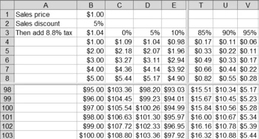
For example, you may want to provide a data table listing retail sales prices and their equivalent sales prices with sales tax added, as shown in Figure 2-3. Cells A3 through A102 list whole dollar amounts from $1.00 to $100.00, while cells B3 through B102 list the correspon-ding whole dollar amounts with sales tax added. So, if the sales tax rate were 8.8%, cell A3 would display $1.00, and cell B3 would display $1.09. Similarly, cell A99 would display $97.00, and cell B99 would display $105.54.

(46)

Going further with this example, you may want to provide a data table listing the same retail prices, but with various discount percentages applied and their equivalent discounted sales prices with sales tax added after that, as shown in Figure 2-4. Cells B4 through B103 list whole dollar amounts from $1.00 to $100.00 as before, but cells C3 through V3 list discount percentages in 5% increments, from 0% to 95%. So, cell B4 would still display $1.00, while cell T4 (an 85% discount) would display $0.17. Similarly, cell A99 would still display $96.00, while cell E99 (a 10% discount) would display $94.01.

Figure 2-3.A data table listing retail sales prices with and without sales tax added (panes split

for readability)

Figure 2-4.A data table listing retail sales prices with discounts and sales tax added (panes split

(47)

How Do I Create Data Tables?

To create data tables, you need to understand the two types of data tables. You should also be familiar with how data tables are constructed with input and output data in various worksheet cells.

You can create either one-variable or two-variable data tables. The difference is in the number of input valuescontained in the table. In a one-variable data table, input values consist of one input cell. In a two-variable data table, input values consist of two input cells. These input cells contain the replaceable values in the formula that are substituted from the row or column input values (for one-variable data tables) or the row and column input val-ues (for two-variable data tables).

Data tables also contain result values. Result values are, as the name suggests, the results of substituting the input values in the formula.

For example, in the data table in Figure 2-5, cells B1 and B2 are the input cells, cells B4 through B13 are the column input values, cells C3 through L3 are the row input values, and cells C4 through L13 (the cells with the values 1.4 through 14.1) are the result values.

Now that you understand data tables terminology, you will learn how to work with one-variable and two-variable data tables.

Working with One-Variable Data Tables

You must organize the data on your worksheets in a certain way in order for Excel to properly create data tables. You design one-variable data tables so that input values are listed either down a column or across a row. A formula used in a one-variable data table must refer to a single input cell.

Figure 2-5.A data table listing values according to the Pythagorean Theorem,

(48)

Here’s the general procedure for setting up and creating a one-variable data table:

1. Type the formula in the appropriate location:

• If the input values are listed down a column, type the formula in the row above the first column value, and then one cell to the right of the column of values. • If the input values are listed across a row, type the formula in the column one cell

below the row of values.

2. Select the group of cells that contains the formula and input values that you want to substitute.

3. Click Data ➤Table.

4. Identify the input cell reference:

• If the input values are listed down a column, type or click the input cell reference in the Column Input box.

• If the input values are listed across a row, type or click the input cell reference in the Row Input box.

5. Click OK.

For example, Figure 2-6 shows how to set up a one-variable data table with input values down a column. Notice that the formula is in the cell above and then to the right of the first column input value. Cell B1 and cells A3 through A12 contain the number of free airline trips. Cell B2 holds the formula =B1*25000. The data table automatically calculates the values in cells B3 through B12.

Figure 2-7 shows how to set up a one-variable data table with input values across a row. Notice that the formula is in the cell below the first row input value. Cells B1 through K1 con-tain the number of free airline trips. Cell B2 concon-tains the formula =B1*25000. The data table automatically calculates the values in cells C2 through K2.

(49)

Working with Two-Variable Data Tables

Unlike one-variable data tables, two-variable data tables’ input values are listed both down a column and across a row. A formula used in a two-variable data table refers to two different input cells.

Here’s the general procedure for setting up and creating a two-variable data table:

1. Type the formula that will serve as the basis of the two-variable data table.

2. Type the list of column input values below the formula in the same column.

3. Type the list of row input values in the same row as the formula, just to the right of the formula.

4. Select the group of cells that contains the formula and the column and row of input values that you want to substitute.

6. In the Column Input box, type or click the column input cell reference.

7. In the Row Input box, type or click the row input cell reference.

8. Click OK.

For example, Figure 2-8 shows how to set up a two-variable data table. In this example, the formula is the sum of basketball free throws and field goals made multiplied by the points for each free throw and field goal. Notice that the list of column input values begins below the formula in the same column as the formula. The list of row input values begins in the same row as the formula, just to the right of the formula.

Figure 2-7.Setting up a one-variable data table with input values across a row (panes split

(50)

Clearing Data Tables

After you create a data table, you may discover that you entered the wrong input cell references, and you want to re-create the data table. Here’s how to do this:

1. Select all of the data table’s result values.

2. Click Edit ➤Clear ➤Contents.

3. Create the data table again.

If you want to clear an entire data table, including the formula, the input cells, the input values, and the result values, follow these steps:

1. Select the entire data table, including all formulas, input cells, input values, and result values.

2. Click Edit ➤Clear ➤All.

Converting Data Tables

You may want to convert formula result values into constant values (in other words, to remove the formulas from result value cells). Here’s how to do this:

1. Select all of the data table’s result values.

2. Click Edit ➤Copy.

3. Click Edit ➤Paste Special.

4. Click the Values option.

5. Click OK.

6. Press Enter.

(51)

Adjusting Data Table Calculation Options

If you recalculate the values in a workbook and the workbook contains data tables, by default, the data tables’ result values will be recalculated as well, even if the result values themselves have not changed. This results in slower overall recalculation performance for the workbook. To speed up recalculations for a workbook that contains data tables, follow these steps:

1. Click Tools ➤Options, and then click the Calculation tab.

2. Click the Automatic Except Tables option.

3. Click OK.

■

Note

To manually recalculate a data table later, click the data table’s formula, and then press F9 (to recal-culate all worksheets in all open workbooks) or press Shift+F9 (to recalrecal-culate only the active worksheet).

Now that you know how to create data tables, practice using them in the following Try It exercises.

Try It: Use Data Tables to Forecast Savings

Account Details

In this exercise, you will use one-variable and two-variable data tables to forecast savings account financial details. These exercises are included in the Excel workbook named Data Tables Try It Exercises.xls, which is available for download from the Source Code area of the Apress web site (http://www.apress.com). This exercise’s data tables are on the workbook’s One-Variable Interest Rates and Two-Variable Interest Rates worksheets.

Notice that on these two worksheets, cells B1 through B4 contain the initial input data, as follows:

• Cell B1 represents the initial savings account investment. • Cell B2 represents the interest rate, compounded monthly. • Cell B3 represents the savings term in months.

• Cell B4 represents the ending savings account value, expressed using the function

=FV(Rate, Nper, , Pv). In this function, Rateis the interest rate (cell B2 divided by 12),

(52)

One-Variable Data Table to Forecast Savings Account Details

To create the one-variable data table, start with the data on the One-Variable Interest Rates worksheet, as shown in Figure 2-9.

Next, determine what the ending savings account value would be for initial investment amounts of $100.00 to $1,000.00, in $100.00 increments. Do the following to create the data table and format the results:

1. In cell A5, type 100.

2. Select cells A5 through A14.

3. Click Edit ➤Fill ➤Series.

4. In the Step Value box, type 100.

5. Click OK.

6. Select cells A4 through B14.

8. In the Column Input Cell box, type or click cellB1.

9. Click OK.

10. Select cells A5 through B14.

11. Click Format ➤Cells.

12. Click Currency in the Category list.

13. Click OK.

Compare your results to Figure 2-10.

Figure 2-9.Initial data before creating the one-variable data table to forecast savings account

financial details

Figure 2-10.Completed

(53)

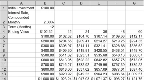
Two-Variable Data Table to Forecast Savings Account Details

To create the two-variable data table, start with the data on the Two-Variable Interest Rates worksheet. The initial data looks just like the data in the One-Variable Interest Rates work-sheet, shown earlier in Figure 2-9.

Next, determine what the ending savings account value would be for initial investment amounts of $100.00 to $1,000.00, in $100.00 increments and savings terms of 12 months to 60 months. Do the following to create the data table and format the results:

1. In cell B5, type 100.

2. Select cells B5 through B14.

5. Click OK.

6. In cell C4, type 12.

7. Select cells C4 through G4.

9. In the Step Value box, type 12.

10. Click OK.

11. Select cells B4 through G14.

12. Click Data ➤Table.

13. In the Row Input Cell box, type or click cell B3.

14. In the Column Input Cell box, type or click cell B1.

15. Click OK.

16. Select cells B5 through G14.

19. Click OK.

(54)

Now try using one-variable and two-variable data tables to determine artist royalty payments.

Try It: Use Data Tables to Determine Royalty

Payments

In this exercise, you will create one-variable and two-variable data tables to determine music artist royalty payments. These exercises are available on the Data Tables Try It Exercises.xls workbook’s One-Variable Royalty Payments and Two-Variable Royalty Payments worksheets.

• Cell B1 represents the recording units’ suggested retail price.

• Cell B2 represents the units’ wholesale price expressed as a percentage of the suggested retail price.

• Cell B3 represents the artist’s royalty rate expressed as a percentage. • Cell B4 represents the number of recording units sold.

• Cell B5 represents the artist’s royalty, using the simple formula B1*B2*B3*B4.

(55)

One-Variable Data Table to Determine Royalty Payments

To create the one-variable data table, start with the data on the One-Variable Royalty Payments worksheet, as shown in Figure 2-12.

Next, determine what the artist’s royalty payments would be for recording units sold of 10,000 to 100,000, in 10,000-unit increments. Do the following to create the data table and format the results:

1. In cell A6, type 10000.

5. Click OK.

8. In the Column Input Cell box, type or click cell B4.

9. Click OK.

10. Select cells B6 through B15.

13. Click OK.

Figure 2-12.Initial data before creating the one-variable data table to determine artist royalty

(56)

Two-Variable Data Table to Determine Royalty Payments

To create the two-variable data table, start with the data on the Two-Variable Royalty Payments worksheet. The initial data looks just like the data in the One-Variable Royalty Payments work-sheet, shown earlier in Figure 2-12.

Next, determine what the artist’s royalty payments would be for recording units sold of 10,000 to 100,000, in 10,000-unit increments and artist royalty percentages from 8% to 10% in 0.5% increments. Do the following to create the data table and format the results:

1. In cell B6, type 10000.

2. Select cells B6 through B15.

5. Click OK.

6. Type the following values in the following cells: C5: 8.0%

D5: 8.5%

E5: 9.0%

F5: 9.5%

G5: 10.0%

7. Select cells B5 through G15.

(57)

9. In the Row Input Cell box, type or click cell B3.

10. In the Column Input Cell box, type or click cell B4.

11. Click OK.

12. Select cells C6 through G15.

15. Click OK.

■

Note

The initial number of units sold in cell B4 of Figures 2-13 and 2-14 and the initial artist royalty rate in cell B3 of Figure 2-14 can be any value. These values are used initially to form the worksheet function in cell B5 of Figures 2-13 and 2-14. However, the data tables substitute these initial values with the values in cells A6 through A15 in Figure 2-13, and cells B6 through B15 and cells C5 through G5 in Figure 2-14.

Now try using one-variable and two-variable data tables to calculate stock dividend payments.

(58)

Try It: Use Data Tables to Calculate Stock

Dividend Payments

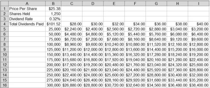
In this exercise, you will create one-variable and two-variable data tables to calculate stock dividend payments. These exercises are available on the Data Tables Try It Exercises.xls work-book’s One-Variable Dividends Payments and Two-Variable Dividends worksheets.

• Cell B1 represents the price per share of stock. • Cell B2 represents the number of shares held.

• Cell B3 represents the dividend rate per share of stock, expressed as a percentage. • Cell B4 represents the total dividends paid, using the simple formula B1*B2*B3.

One-Variable Data Table to Calculate Stock Dividend Payments

To create the one-variable data table, start with the

data on the One-Variable Dividends Payments work-sheet, as shown in Figure 2-15.

Next, determine what the stock dividend pay-ments are for shares of stock held from 25,000 to 300,000, in 25,000-share increments. Do the following to create the data table and format the results:

1. In cell A5, type 25000.

5. Click OK.

8. In the Column Input Cell box, type or click cellB2.

9. Click OK.

10. Select cells B5 through B16.

13. Click OK.