CONTOURS ON ABDOMINAL IMAGE BOUNDARY DETECTION
Cherry Ballangan
Faculty of Industrial Technology, Informatics Engineering Department, Petra Christian University e-mail: [email protected]
ABSTRACT: Active contour, or snake, is an energy minimizing spline that is useful in image boundary detection. Active contours are stimulated by internal forces, image forces and external forces which maintain the shape of the contours while attract the contours to some desired features, usually edges. Problems in implementing active contours such as convergence and initialization have motivated researchers to modify image forces of the active contours. This paper presents a comparative study among three different image forces: traditional snakes, balloon and gradient vector flow (GVF). The study is validated by experiments on abdominal image boundaries detection.These lead to the conclusion that GVF gives the most appropriate results among the other approaches.
Keywords: active contours, snake, balloon, gradient vector flow.
INTRODUCTION
An active contour, developed by Kass et al [1], is a tool for detecting a particular feature (especially edges) in an image. Active contours use energy minimization to impose a contour toward an edge. While the contours minimizing their energy, they slither toward the boundary that make them called
snakes.
The use of active contours has become popular in computer vision such as in image morphing [2], shape modeling [3], image segmentation [4] and image registration [5], and has been studied and modified by many researchers [6-8].
In this paper, a comparative study is presented to investigate the behavior of active contours under different image forces approaches: traditional snakes, balloon and gradient vector flow (GVF). First, the basic theory of active contours followed by the numerical implementation is presented. Then, balloon and GVF are also explained followed by the result of the experiments and a discussion.
ACTIVE CONTOURS
Basics
Active contours are influenced by internal forces, image forces, and external constraint forces. The internal forces serve as a smoothness constraint, keeping the contour from discontinuity or bending too much. The image forces are responsible for attracting the snake to the desired boundary, whereas the external constraint forces are the conditions that are set by the users.
The energy functional is represented mathe-matically by:
( )
( )
∫
=∗ 1
0E vs ds
Esnake snake
=
∫
01Eint( )
v( )
s +Eimage( )
v( )
s +Econ( )
v( )
s ds(1)
Where v(s) = [x(s), y(s)] is a curve and s∈ [0, 1].
• The first term of equation Eq. 1 represents the internal energy responsible for the smoothness and deformation of the contour and is expressed as:
( ) ( )
( ) ( )
(
2 2)
2int s v s s v s
E = α s +β ss
If α =0, discontinuity happened whereas if
0
=
β , the snake will develop a corner.
• The second term of Eq. 1 forces the snake to the true edge of the image. Kass et al presents three different energy functionals, i.e. line, edge and termination, which can be expressed as:
term term edge edge line line
image w E w E w E
E = + +
• The third term of Eq. 1 comes from external
constraints imposed either by a user or some other higher level process which may force the snake toward or away from particular features.
Numerical Implementation
Snake can be implemented numerically in the form of matrix equation:
xt = (A + γI)-1(x t-1 – fx(xt-1,yt-1))
yt = (A + γI)-1(y t-1 – fy(xt-1,yt-1)) (2)
and y axis respectively, γ is a step size and A is a diagonal banded matrix. If a contour is discretised into S points equally spaced by an arc length h and s
For the contour to be converged to the desired edge, an initial contour needs to be placed carefully. This initial contour is then used in Eq. 2 as a start of the deformation. Matrix A can be obtained by using
Eq. 3 where the length of α(s) and β(s) equal to the length of the initial contour.
The next step is calculating fx(x,y) and fy(x,y) to be used in Eq. 2. Let [px, py] be the gradient of the initial contour, then fx(x,y) and fy(x,y) can be obtained by using an interpolation of the boundary specified by the matrices px and py respectively.
ACTIVE CONTOUR MODELS
The active contour model above is very useful since it maintains the shape as a curve and the final form of the contour can be influenced by feedback from a higher level process. Nevertheless, there are some problems in implementing them. One problem that often appears is the difficulty in determining the initial contour which has an important contribution to the success of the real edges detection. Locating the initial contour in a place that is not close to the original contour will make the snake’s convergence go to the wrong result because it will not be pulled toward the original contour.
Some approaches have been proposed by many researchers to solve this problem. Cohen [6]
sugges-ted a method that is called a “balloon”. He claims that the initial contour does not need to be close to the target contour as in the original version of snake. He modifies the original snake by using an inflation force so that the curve reacts like a balloon. The contour will be inflated and pass the weak edges but will be stopped if the edge is strong with respect to the inflation force. This modified image force is presented as
Another effort to solve the problem of initializa-tion and convergences has been performed by Xu et al. [7] by defining a new image force. This image
force field, which is called gradient vector flow
(GVF) is able to move into boundary concavities and can be initialized in quite a distance from the boundary. They defined the GVF as a vector field
v(x, y) = (u(x,y), v(x,y)) that minimizes the energy
where µ is a regularization parameter which should be set according to the amount of noise of the image and f (x, y) is the edge map derived from the image.
EXPERIMENTAL RESULTS
In these experiments, the active contours are used to detect abdominal images boundaries. The initial contours are obtained from the boundary of another corresponding abdominal image.
Firstly, experiments were performed on 5 different abdominal CT (Computed Tomography) images and another series of experiments were carried out on 5 different PET (Positron Emission Tomography) images. Table 1 presents the result of these series of experiments by showing the number of iteration needed for the initial contour to be converged to the true boundary for each approach: traditional snake, GVF, and balloon with force weight parameter 0.05 and 0.01. The image size used in the first five experiments are 512 × 512 pixels, whereas the image size used in the other five experiments are 128 × 128 pixels, which made them converge faster than the previous five experiments.
failed to converge. This will be discussed in the next part.
Table 1.
Number of iteration Images to
be registered
Traditional
snake GVF
Balloon (w=0.05)
Balloon (w=0.01)
CT 1 78 60 22 54
CT 2 168 130 29 99
CT 3 230 218 - 269
CT 4 109 78 32 75
CT 5 246 232 - 275
PET 1 18 11 13 17
PET 2 10 9 10 10
PET 3 16 11 25 18
PET 4 18 12 22 17
PET 5 15 9 25 18
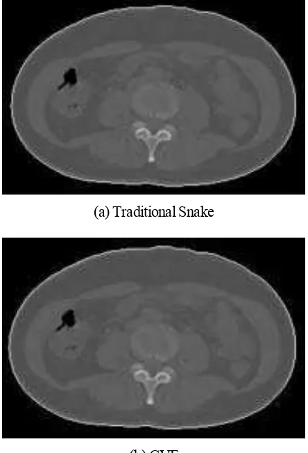
Besides convergence speed, the results between traditional snake, GVF, and balloon approach are comparable. That is because the images used in those experiments are relatively smooth and do not contain a concave shape. The results of the deformed contour for CT 3 in Table 1 are presented in Figure 1. It can be seen that the deformed contours fit perfectly to the true boundary.
(a) Traditional Snake
(b) GVF
(c) Balloon
Figure 1. Results of The Active Contours After Converged.
DISCUSSION
Balloon
The balloon approach had unpredictable results in some experiments. The balloon method works well if the initial contours positioned inside the true boundaries. However, in some cases we need to place the initial contours outside or even crossing the boundaries. For example, for registering two abdo-minal images, the initial contours can be obtained from the first stage of the registration, which are usually located crossing the true boundary.
As shown in Table 1, when the pressure para-meter is set to a higher value, the contour will converge remarkably quickly. However, for some images (e.g. CT 3 and CT 5 in Table 1), when the initial contours positioned outside the boundaries and the distance is quite far, this model failed to converge, since the initial contours tended to expand rather than shrink to the boundaries.
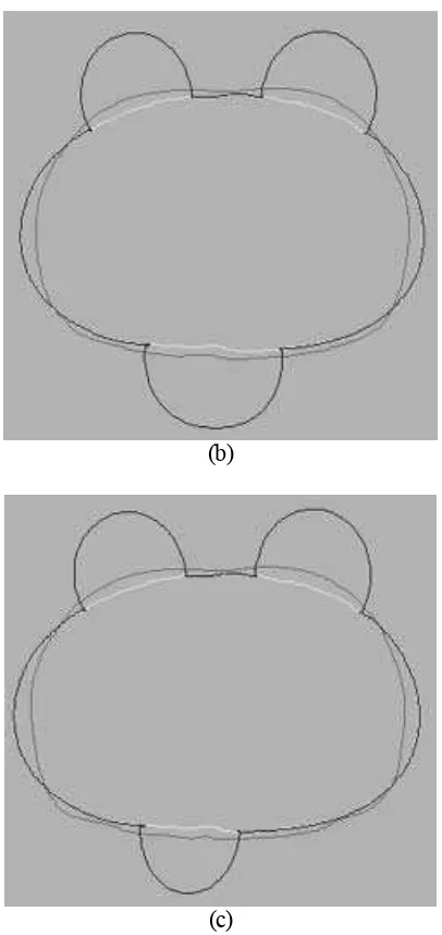
Figure 2 presents the result of balloon approach for CT 1, CT 3 and CT 5 mentioned in Table 1. The magenta contours are the initial contours, the yellow contours are the target boundaries, and the blue contours are the deformed contours after they reached convergence, or after the 500th iteration. Note that in Figure 2(a), the blue contour fits the yellow contour since the initial contour can converge well to the target boundary.
(a)
(b)
(c)
Figure 2. The contours result of Balloon Approach
(a)
(b)
(c)
Figure 3. The contours results of Balloon Approach
If the pressure parameter is set to a lower value, the contour will have behavior that is similar to the traditional snakes, because the expanding force is relatively small. Hence, the choices of the parameters are very important to obtain a good performance and results.
GVF
that GVF encourages convergence to boundary concavities. This cannot be shown by abdominal images
The behavior of the GVF approach that is able to converge to boundary concavity can be explained from the Euler equations used to find the GVF field. These Euler equations are:
(
)
(
2 2)
02 − − + =
∇ u u fx fx fy
µ
( )
(
2 2)
02 − − + =
∇ v v fy fx fy
µ
where ∇2 is the Laplacian operator, f (x, y) is the edge map derived from the image I(x, y), and v(x, y) = (u(x,y), v(x,y)) is the vector field. When I(x, y) is constant, then the gradient of f (x, y) is zero, which means u and v are determined by Laplace’s equation. As a result, the gradient vector field is interpolated from the region’s boundary [7].
CONCLUSION
Some experiments on different active contour approaches, including traditional snake, GVF, and balloon, have been done to compare the performance of each approach. The GVF always perform with faster active contour procedures, compared to traditional snake. Balloon methods sometimes can perform the fastest procedure compared to other approaches. However, the results are somehow unpredictable.
REFERENCES
1. Kass, M., A. Witkin and D. Terzopoulos.
“Snakes: Active Contour Models”. International
Journal of Computer Vision. Vol. 1. 1988. pp. 321-331.
2. Lee, S.-Y., K.-Y. Chwa, S. Y. Shin and G.
“Wolberg. Image Metamorphosis Using Snakes
and Free-Form Deformations”. ACM. 1995. Vol.
pp. 439-448.
3. Wang, H. and B. Ghosh. “Geometric active
deformable models in shape modeling”. IEEE
Transactions on Image Processing. 2000. Vol. 9(2). pp. 302 - 308.
4. Davatzikos, C. A. and J. L. Prince. “An Active
Contour Model for Mapping the Cortex”. IEEE
Transactions on Medical Imaging. Vol. 14(1). 1995. pp. 65-80.
5. King, P., S. Mitra and B. Nutter. “An Automated, Segmentation-Based, Rigid Registration System
For Cervigram/Spl Trade/Images Utilizing Simple Clustering and Active Contour Techniques”. 17th IEEE Symposium on Computer-Based Medical Systems. Proceedings. 2004. pp. 292-297.
6. Cohen, L. D. “On active contour models and
balloons”. Computer Vision, Graphics, and Image Processing: Image Understanding. Vol. 53(2). 1991. pp. 211-218.
7. Xu, C. and J. L. Prince. “Snakes, Shapes, and
Gradient Vector Flow”. IEEE Transactions on
Image Processing. Vol. 7(3). 1998. pp. 359-369.
8. Segonne, F., J. P. Pons, B. Fischl and E. Grimson. A Novel Active Contour Framework: Multi-component Level Set Evolution under Topology Control. 2005.
9. Nixon, M. and A. Aguado. Feature Extraction