Full Terms & Conditions of access and use can be found at
http://www.tandfonline.com/action/journalInformation?journalCode=ubes20
Download by: [Universitas Maritim Raja Ali Haji] Date: 11 January 2016, At: 22:59
Journal of Business & Economic Statistics
ISSN: 0735-0015 (Print) 1537-2707 (Online) Journal homepage: http://www.tandfonline.com/loi/ubes20
Evaluating Value-at-Risk Models via Quantile
Regression
Wagner Piazza Gaglianone, Luiz Renato Lima, Oliver Linton & Daniel R.
Smith
To cite this article: Wagner Piazza Gaglianone, Luiz Renato Lima, Oliver Linton & Daniel R. Smith (2011) Evaluating Value-at-Risk Models via Quantile Regression, Journal of Business & Economic Statistics, 29:1, 150-160, DOI: 10.1198/jbes.2010.07318
To link to this article: http://dx.doi.org/10.1198/jbes.2010.07318
Published online: 01 Jan 2012.
Submit your article to this journal
Article views: 610
View related articles
Evaluating Value-at-Risk Models via
Quantile Regression
Wagner Piazza GAGLIANONE
Research Department, Central Bank of Brazil and Fucape Business School, Brasília DF 70074-900, Brazil (wagner.gaglianone@bcb.gov.br)
Luiz Renato LIMA
Department of Economics, University of Tennessee at Knoxville and EPGE-FGV, 527A Stokely Management Center, Knoxville, TN 37996-0550 (llima@utk.edu)
Oliver LINTON
Department of Economics, London School of Economics, Houghton Street, London WC2A 2AE, United Kingdom (o.linton@lse.ac.uk)
Daniel R. SMITH
Faculty of Business Administration, Simon Fraser University, 8888 University Drive, Burnaby BC V6P 2T8, Canada and School of Economics and Finance, Queensland University of Technology, Brisbane Q 4001, Australia
(drsmith@sfu.ca;dr.smith@qut.edu.au)
This article is concerned with evaluating Value-at-Risk estimates. It is well known that using only binary variables, such as whether or not there was an exception, sacrifices too much information. However, most of the specification tests (also called backtests) available in the literature, such as Christoffersen (1998) and Engle and Manganelli (2004) are based on such variables. In this article we propose a new backtest that does not rely solely on binary variables. It is shown that the new backtest provides a sufficient condition to assess the finite sample performance of a quantile model whereas the existing ones do not. The proposed methodology allows us to identify periods of an increased risk exposure based on a quantile regression model (Koenker and Xiao2002). Our theoretical findings are corroborated through a Monte Carlo simulation and an empirical exercise with daily S&P500 time series.
KEY WORDS: Backtesting; Risk exposure.
1. INTRODUCTION
Recent financial disasters emphasized the need for accurate risk measures for financial institutions. Value-at-Risk (VaR) models were developed in response to the financial disasters of the early 1990’s, and have become a standard measure of mar-ket risk, which is increasingly used by financial and nonfinan-cial firms as well. In fact, VaR is a statistical risk measure of po-tential losses, and summarizes in a single number the maximum expected loss over a target horizon at a particular significance level. Despite several other competing risk measures proposed in the literature, VaR has effectively become the cornerstone of internal risk management systems in financial institutions, following the success of the J. P. Morgan (1996) RiskMetrics system, and nowadays form the basis of the determination of market risk capital, since the 1996 Amendment of the Basel Accord.
Another advantage of VaR is that it can be seen as a coherent risk measure for a large class of continuous distributions, that is, it satisfies the following properties: (i) subadditivity (the risk measure of a portfolio cannot be greater than the sum of the risk measures of the smaller portfolios that comprise it); (ii) ho-mogeneity (the risk measure is proportional to the scale of the portfolio); (iii) monotonicity (if portfolioYdominatesX, in the sense that each payoff ofYis at least as large as the correspond-ing payoff ofX, i.e.,X≤Y, thenX must be of lesser or equal risk); and (iv) risk-free condition (adding a risk-free instrument
to a portfolio decreases the risk by the size of the investment in the risk-free instrument).
Daníelsson et al. (2005) and Ibragimov and Walden (2007) showed that for continuous random variables either VaR is co-herent and satisfies subadditivity or the first moment of the in-vestigated variable does not exist. In this sense, they showed that VaR is subadditive for the tails of all fat distributions, pro-vided the tails are not super fat (e.g., Cauchy distribution). In this way, for a very large class of distributions of continuous random variables, one does not have to worry about subadditiv-ity violations for a VaR risk measure.
A crucial issue that arises in this context is how to eval-uate the performance of a VaR model. According to Giaco-mini and Komunjer (2005), when several risk forecasts are available, it is desirable to have formal testing procedures for comparison, which do not necessarily require knowledge of the underlying model, or if the model is known, do not re-strict attention to a specific estimation procedure. The litera-ture proposed several tests (also known as “backtests”), such as Kupiec (1995), Christoffersen (1998), and Engle and Man-ganelli (2004), mainly based on binary variables (i.e., an in-dicator for whether the loss exceeded the VaR), from which
© 2011American Statistical Association Journal of Business & Economic Statistics
January 2011, Vol. 29, No. 1 DOI:10.1198/jbes.2010.07318
150
statistical properties are derived and further tested. More re-cently, Berkowitz, Christoffersen, and Pelletier (2009) devel-oped a unified framework for VaR evaluation and showed that the existing backtests can be interpreted as a Lagrange multi-plier (LM)-type of tests.
The existing backtests are based on orthogonality conditions between a binary variable and some instruments. If the VaR model is correctly specified, then this orthogonality condition holds and one can, therefore, use it to derive an LM test. Monte Carlo simulations showed that such tests have low power in fi-nite samples against a variety of misspecified models. The prob-lem arises because binary variables are constructed to represent rare events. In finite samples, it may be the case that there are few extreme events, leading to a lack of the information needed to reject a misspecified model. In this case, a typical solution will be to either increase the sample size or construct a new test that uses more information than the existing ones to reject a misspecified model.
The contribution of this article is twofold. First, we propose a random coefficient model that can be used to construct a Wald test for the null hypothesis that a given VaR model is correctly specified. To the best of our knowledge no such framework ex-ists in the current literature. It is well known that although LM and Wald tests are asymptotically equivalent under the null hy-pothesis and local alternatives, they can yield quite different re-sults in finite samples. We show in this article that the new test uses more information to reject a misspecified model, which makes it deliver more power in finite samples than any other existing test.
Another limitation of the existing tests is that they do not give any guidance as to how the VaR models are wrong. The sec-ond contribution of this article is to develop a mechanism by which we can evaluate the local and global performances of a given VaR model, and therefore, find out why and when it is misspecified. By doing this we can unmask the reasons of re-jection of a misspecified model. This information can be used to reveal if a given model is underestimating or overestimat-ing risk, if it reacts quickly to increases in volatility, or even to suggest possible model combinations that will result in more accurate VaR estimates. Indeed, it was proven that model com-bination (see Issler and Lima2009) can increase the accuracy of forecasts. Since VaR is simply a conditional quantile, it is also possible that model combination can improve the fore-cast of a given conditional quantile or even of an entire den-sity.
Our Monte Carlo simulations as well as our empirical ap-plication using the S&P500 series corroborate our theoretical findings. Moreover, the proposed test is quite simple to compute and can be carried out using software available for conventional quantile regression, and is applicable even when the VaR does not come from a conditional volatility model.
This study is organized as follows: Section2defines Value-at-Risk and the model we use, Section3 presents a quantile regression-based hypothesis test to evaluate VaRs. In Section4, we briefly describe the existing backtests and establish a suffi-cient condition to assess a quantile model. Section5shows the Monte Carlo simulation comparing the size and power of the competing backtests. Section6presents a local analysis of VaR models and Section7provides an empirical exercise based on daily S&P500 series. Section8concludes.
2. THE MODEL
A Value-at-Risk model reports the maximum loss that can be expected, at a particular significance level, over a given trad-ing horizon. The VaR is defined by regulatory convention with a positive sign (following the Basel accord and the risk man-agement literature). If Rt denotes the return of a portfolio at
timet, and τ∗∈(0,1)denotes a (predetermined) significance level, then the respective VaR (Vt) is implicitly defined by the
following expression:
Pr[Rt<−Vt|Ft−1] =τ∗, (1)
whereFt−1is the information set available at timet−1. From the above definition it is clear that−Vtis theτ∗th conditional
quantile ofRt. In other words,−Vt is the one-step ahead
fore-cast of theτ∗th quantile ofRt based on the information
avail-able up to periodt−1.
From Equation (1) it is clear that finding a VaR is equivalent to finding the conditional quantile ofRt. Following the idea of
Christoffersen, Hahn, and Inoue (2001), one can think of gen-erating a VaR measure as the outcome of a quantile regression, treating volatility as a regressor. In this sense, Engle and Pat-ton (2001) argued that a volatility model is typically used to forecast the absolute magnitude of returns, but it may also be used to predict quantiles. In this article, we adapt the idea of Christoffersen, Hahn, and Inoue (2001) to investigate the ac-curacy of a given VaR model. In particular, instead of using the conditional volatility as a regressor, we simply use the VaR measure of interest (Vt). We embed this measure in a general
class of models for stock returns in which the specification that deliveredVtis nested as a special case. In this way, we can
pro-vide a test of the VaR model through a conventional hypothesis test. Specifically, we consider that there is a random coefficient model forRt, generated in the following way:
Rt=α0(Ut)+α1(Ut)Vt (2)
=x′tβ(Ut), (3)
where Vt is Ft−1-measurable in the sense that it is already
known at period t −1, Ut ∼iid U(0,1), and αi(Ut), i =
0,1, are assumed to be comonotonic in Ut, with β(Ut)= [α0(Ut), α1(Ut)]′andx′t= [1,Vt].
Proposition 1. Given the random coefficient model in Equa-tion (2) and the comonotonicity assumption ofαi(Ut),i=0,1,
theτth conditional quantile ofRtcan be written as
QRt(τ|Ft−1)=α0(τ )+α1(τ )Vt for allτ∈(0,1). (4)
Proof. SeeAppendix.
Now, recall what we really want to test Pr(Rt < −Vt|
Ft−1)=τ∗, that is,−Vtis indeed theτ∗th conditional quantile
ofRt. Therefore, considering the conditional quantile model in
Equation (4), a natural way to test for the overall performance of a VaR model is to test the null hypothesis
Ho:
The null hypothesis can be presented in a classical formula-tion asHo:Wβ(τ∗)=r, for the fixed significance level
(quan-tile) τ =τ∗, where W is a 2×2 identity matrix; β(τ∗)=
[α0(τ∗), α1(τ∗)]′ andr= [0,−1]′. Note that, due to the sim-plicity of our restrictions, the latter null hypothesis can still be reformulated as Ho:θ (τ∗)=0, where θ (τ∗)= [α0(τ∗),
(α1(τ∗)+1)]′. Notice that the null hypothesis should be inter-preted as a Mincer and Zarnowitz (1969)-type regression frame-work for a conditional quantile model.
3. THE TEST STATISTIC AND ITS NULL DISTRIBUTION
Let θ (τ∗) be the quantile regression estimator of θ (τ∗).
The asymptotic distribution ofθ (τ∗)can be derived following Koenker (2005, p. 74), and it is normal with covariance matrix that takes the form of a Huber (1967) sandwich:
√
computed by using, for instance, the techniques in Koenker and Machado (1999). Given that we are able to compute the co-variance matrix of the estimatedθ (τ )coefficients, we can now construct our hypothesis test to verify the performance of the Value-at-Risk model based on quantile regressions (hereafter, VQR test).
Definition 1. Let our test statistic be defined by
ζVQR=T
θ (τ∗)′(τ∗(1−τ∗)Hτ−∗1JHτ−∗1)−1θ (τ∗). (7) In addition, consider the following assumptions:
Assumption 1. Letxtbe measurable with respect toFt−1and
zt≡ {Rt,xt}be a strictly stationary process.
Assumption 2 (Density). Let Rt have conditional (on xt)
distribution functions Ft, with continuous Lebesgue
densi-ties ft uniformly bounded away from 0 and ∞ at the points QRt(τ|xt)=F−
1
t (τ|xt)for allτ∈(0,1).
Assumption 3(Design). There exist positive definite matri-cesJandHτ, such that for allτ∈(0,1):
The asymptotic distribution of the VQR test statistic, un-der the null hypothesis thatQRt(τ∗|Ft−1)= −Vt, is given by
Proposition2, which is merely an application of Hendricks and Koenker (1992) and Koenker (2005, theorem 4.1) for a fixed quantileτ∗.
Proposition 2(VQR test). Consider the quantile regression in Equation (4). Under the null hypothesis in Equation (5), if Assumptions1through4 hold, then, the test statisticζVQR is asymptotically chi-squared distributed with 2 degrees of free-dom.
Proof. SeeAppendix.
Remark 1. Assumption 1 together with comonotonicity of
αi(Ut),i=0,1, guarantee the monotonic property of the
condi-tional quantiles. We recall the comment of Robinson (2006), in which the author argues that comonotonicity may not be suffi-cient to ensure monotonic conditional quantiles, in cases where
xt can assume negative values. In our case, xt≥0.
Assump-tion2relaxes the iid assumption in the sense that it allows for nonidentical distributions. Bounding the quantile function esti-mator away from 0 and∞is necessary to avoid technical com-plications. Assumptions2 through4 are quite standard in the quantile regression literature (e.g., Koenker and Machado1999 and Koenker and Xiao2002) and familiar throughout the liter-ature onM-estimators for regression models, and are crucial to apply the central limit theorem (CLT) of Koenker (2005, theo-rem 4.1).
Remark 2. Under the null hypothesis it follows that−Vt= QRt(τ∗|Ft−1), but under the alternative hypothesis the random
nature ofVt, captured in our model by the estimated coefficients
θ (τ∗)=0, can be represented by −Vt=QRt(τ∗|Ft−1)+ηt,
whereηt represents the measurement error of the VaR on
esti-mating the latent variableQRt(τ∗|Ft−1). Note that Assumptions 1through4are easily satisfied under the null and the alterna-tive hypotheses. In particular, note that Assumption4underH1 implies that alsoηtis bounded.
Remark 3. Assumptions 1 through 4 do not restrict our methodology to those cases in which Vt is constructed from
a conditional volatility model. Indeed, our methodology can be applied to a broad number of situations, such as:
(i) The model used to constructVtis known. For instance,
a risk manager trying to construct a reliable VaR measure. In such a case, it is possible that: (ia) Vt is generated from a
conditional volatility model, e.g., Vt =g(σt2), where g(·) is
some function of the estimated conditional varianceσt2, say from a generalized autoregressive conditional heteroscedas-ticity (GARCH) model; or (ib) Vt is directly generated, for
instance, from a conditional autoregressive value at risk by regression (CAViaR) model or an autoregressive conditional heteroscedasticity (ARCH)-quantile method (see Koenker and Zhao1996and Wu and Xiao2002for further details).
(ii) Vt is generated from an unknown model, and the only
information available is{Rt,Vt}. In this case, we are still able
to apply Proposition2as long as Assumptions1through4hold. This might be the case described in Berkowitz and O’Brien (2002), in which a regulator investigates the VaR measure re-ported by a supervised financial institution.
(iii) Vt is generated from an unknown model, but besides {Rt,Vt}a confidence interval of Vt is also reported. Suppose
that a sequence {Rt,Vt,Vt,Vt} is known, in which Pr[Vt < Vt<Vt|Ft−1] =δ, where[Vt,Vt]are, respectively, lower and
upper bounds ofVt, generated (for instance) from a bootstrap
procedure, with a confidence level δ (see Christoffersen and
Goncalves2005; Hartz, Mittnik, and Paolella2006; and Pas-cual, Romo, and Ruiz2006). One can use this additional infor-mation to investigate the considered VaR by making a connec-tion between the confidence interval ofVt and the previously
mentioned measurement errorηt. The details of this route
re-main an issue to be further explored.
4. EXISTING BACKTESTS
Recall that a correctly specified VaR model at level τ∗ is nothing other than theτ∗th conditional quantile ofRt. The goal
of the econometrician is to test the null hypothesis that−Vt
correctly approximates the conditional quantile for a specified levelτ∗. In this section, we review some of the existing back-tests, which are based on an orthogonality condition between a binary variable and some instruments. This framework is the basis of generalized method of moments (GMM) estimation and offers a natural way to construct a Lagrange multiplier (LM) test. Indeed, the current literature on backtesting is mostly represented by LM-type of tests. In finite samples, the LM test and the Wald test proposed in this article can perform quite dif-ferently. In particular, we will show that the test proposed in this article considers more information than some of the ex-isting tests, and therefore, it can deliver more power in finite sample.
We first define a violation sequence by the following indica-tor function or hit sequence:
By definition, the probability of violating the VaR should al-ways be
Pr(Ht=1|Ft−1)=τ∗. (9) Based on these definitions, we now present some backtests usu-ally mentioned in the literature to identify misspecified VaR models:
(i) Kupiec (1995): One of the earliest proposed VaR backtests is due to Kupiec (1995), who proposed a nonparametric test based on the proportion of exceptions. Assume a sample size ofT observations and a number of violations ofN=Tt=1Ht.
The objective of the test is to know whetherp≡N/Tis statis-tically equal toτ∗:
Ho:p=E(Ht)=τ∗. (10)
The probability of observingNviolations over a sample size ofTis driven by a Binomial distribution and the null hypothesis
Ho:p=τ∗can be verified through a likelihood ratio (LR) test
(also known as the unconditional coverage test). This test re-jects the null hypothesis of an accurate VaR if the actual fraction of VaR violations in a sample is statistically different thanτ∗. However, Kupiec (1995) found that the power of his test was generally low in finite samples, and the test became more pow-erful only when the number of observations is very large.
(ii) Christoffersen (1998): The unconditional coverage prop-erty does not give any information about the temporal depen-dence of violations, and the Kupiec (1995) test ignored condi-tioning coverage since violations can cluster over time, which should also invalidate a VaR model. In this sense, Christoffersen
(1998) extended the previous LR statistic to specify that the hit sequence should also be independent over time. The author ar-gued that we should not be able to predict whether the VaR will be violated since if we could predict it, then that information can be used to construct a better risk model. The proposed test statistic is based on the mentioned hit sequenceHt, and onTij
that is defined as the number of days in which a statejoccurred in one day, while it was at state i the previous day. The test statistic also depends onπi, which is defined as the
probabil-ity of observing a violation, conditional on stateithe previous day. It is also assumed that the hit sequence follows a first order Markov sequence with transition matrix given by
=
Note that under the null hypothesis of independence, we have thatπ=π0=π1=(T01+T11)/T, and the following LR
sta-The joint test, also known as the “conditional coverage test,” includes the unconditional coverage and independence proper-ties. An interesting feature of this test is that a rejection of the conditional coverage may suggest the need for improvements on the VaR model to eliminate the clustering behavior. On the other hand, the proposed test has a restrictive feature since it only takes into account the autocorrelation of order 1 in the hit sequence.
Berkowitz, Christoffersen, and Pelletier (2009) extended and unified the existing tests by noting that the de-meaned viola-tions Hitt =Ht−τ∗ form a martingale difference sequence
(mds). By the definition of the violation, Equations (8) and (9) imply that
E[Hitt|Ft−1] =0,
that is, the de-meaned violations form an mds with respect to Ft−1. This implies thatHittis uncorrelated at all leads and lags.
In other words, for any vectorXtinFt−1we must have
E[Hitt⊗Xt] =0, (13)
which constitutes the basis of GMM estimation. The frame-work based on such orthogonality conditions offers a natural way to construct an LM test. Indeed, if we allowXt to include
lags ofHitt,Vtand its lags, then we obtain the well-known
dy-namic conditional quantile (DQ) test proposed by Engle and Manganelli (2004), which we describe below.
(iii) Engle and Manganelli (2004) proposed a new test that in-corporates a variety of alternatives. Using the previous notation, the random variableHitt=Ht−τ∗is defined by the authors, to
construct the DQ test, which involves the following statistic:
DQ=(Hit′tXt[X′tXt]−1X′tHitt)/(Tτ (1−τ )), (14)
where the vector of instrumentsXt might include lags ofHitt, Vt, and its lags. This way, Engle and Manganelli (2004) tested
the null hypothesis thatHittandXtare orthogonal. Under their
null hypothesis, the proposed test statistic follows a χq2, in
whichq=rank(Xt). Note that the DQ test can be used to
eval-uate the performance of any type of VaR methodology (and not only the CAViaR family, proposed in their article).
Several other related procedures can be immediately derived from the orthogonality condition in Equation (13). For exam-ple, Christoffersen and Pelletier (2004) and Haas (2005) pro-posed duration-based tests to the problem of assessing VaR accuracy. However, as shown by the Monte Carlo experiment in Berkowitz, Christoffersen, and Pelletier (2009), the DQ test in which Xt=Vt appears to be the best backtest for 1% VaR
models and other backtests generally have much lower power against misspecified VaR models. In the next section, we pro-vide a link between the proposed VQR test and the DQ test, and we give some reasons that suggest the VQR test should be more powerful than the DQ test in finite samples.
4.1 DQ versus VQR Test
In the previous section we showed that the DQ test pro-posed by Engle and Manganelli (2004) can be interpreted as an LM test. The orthogonality condition in Equation (13) con-stitutes the basis of GMM estimation, and therefore, can be used to estimate the quantile regression model in Equation (4) under the null hypothesis in Equation (5). It is well known that ordinary least squares (OLS) and GMM are asymptoti-cally equivalent. By analogy, quantile regression estimation and GMM estimation are also known to be asymptotically equiva-lent (see, for instance, footnote 5 of Buchinsky1998, and the proofs of Powell1984). However, if the orthogonality condi-tion in Equacondi-tion (13) provides a poor finite sample approxi-mation of the objective function, then GMM and quantile re-gression estimation will be quite different and the LM tests and Wald test proposed in this article will yield very different results. To compare the DQ test and our VQR test, we con-sider the simplest case in which Xt =[1 Vt]′. As shown in
Koenker (2005, pp. 32–37), the quantile regression estimator minimizes the objective function R(β)=nt=1ρτ(yt−Xt′β),
whereρτ(u)=τu1(u≥0)+(τ−1)u1(u<0). Notice thatρτ is a piecewise linear and continuous function, and it is differ-entiable except at the points at which one or more residuals are zero. At such points,R(β)has directional derivatives in all di-rections. The directional derivative ofRin directionwis given by▽R(β,w)= −nt=1ψ (yt−Xt′β,−Xt′w)Xt′w, where then β0 minimizes R(β). Now, consider the quantile prob-lem on which the VQR is based. Therein, if we set yt =Rt, Hit is the same one defined by Engle and Manganelli (2004) and thatHitt=Hit∗t. According to Koenker (2005), there will
be at least p zero residuals where p is the dimension of β. This suggests that the orthogonality conditionn−1nt=1Hitt⊗
[1 Vt]′=0, does not imply▽R(β0,w)≥0 for allw∈R2with
w =1. In this case, the orthogonality condition is not suffi-cient to assess a performance of a quantile modelVt in finite
samples. In practice, the VQR test is using more information than the DQ test to reject a misspecified model, and therefore, it can exhibit superior power in finite samples than the DQ test. Finally, it is possible to generalize this result for a list of in-struments larger thanXt=[1 Vt]′ as long as we redefine our
quantile regression in Equation (4) to include other regressors besides an intercept andVt.
Although the first order conditions n−1nt=1Hitt ⊗
[1 Vt]′=0 do not strictly imply in the optimality condition
▽R(β0,w)≥0 in finite samples, this does not prevent it from holding asymptotically if one makes an assumption that the percentage of zero residuals isop(1)(see the discussion in the
handbook chapter of Newey and McFadden1994). Hence, the DQ test proposed by Engle and Manganelli (2004) and our VQR test are asymptotically equivalent under the null hypoth-esis and local alternatives. However, in finite samples the or-thogonality and the optimality conditions can be quite different and the two tests can, therefore, yield very different results.
Finally, notice that if ▽R(β0,w)≥0 for all w∈R2 with
w =1, then n−1nt=1Hitt ⊗[1 Vt]′ =0. Therefore, the
DQ test is implied by the VQR when the VaR model is cor-rectly specified. Intuitively, this happens because, if −Vt = QRt(τ∗|Ft−1), thenVt will provide a filter to transform a
(pos-sibly) serially correlated and heteroscedastic time series into a serially independent sequence of indicator functions.
In sum, the above results suggest that there are some reasons to prefer the VQR test over the DQ test since the former can have more power in finite samples and be equivalent to the latter under the null hypothesis. A small Monte Carlo simulation is conducted in Section5 to verify these theoretical findings as well as to compare the VQR test with the existing ones in terms of power and size.
5. MONTE CARLO SIMULATION
In this section we conduct a simulation experiment to in-vestigate the finite sample properties of the VQR test. In par-ticular, we are interested in showing under which conditions our theoretical findings are observed in finite samples. We con-sider, besides the VQR test, the unconditional coverage test of Kupiec (1995), the conditional coverage test of Christoffersen (1998), and the out-of-sample DQ test of Engle and Manganelli (2004) in which we adopted the instrumentsXt=[1 Vt]′. We
look at the one-day-ahead forecast and simulate 5000 sample paths of lengthT +Te observations, using the firstTe=250
observations to compute the initial values of Equation (18) with
T= {250;500;1000;2500}(i.e., approximately 1, 2, 4, and 10 years of daily data).
Asymptotic critical values are used in this Monte Carlo ex-periment, but bootstrap methods can also be considered to com-pute finite-sample critical values. For example, for the VQR test we can employ the bootstrap method proposed by Parzen, Wei, and Ying (1994). For the Kupiec, Christoffersen, and DQ tests, finite-sample critical values can be computed by using the method proposed by Dufour (2006). Bootstrap-based critical
values are more difficult to be computed by a financial institu-tion on a daily basis. On the other hand, asymptotic critical val-ues may not be accurate enough in small samples. As the results in this section show, asymptotic critical values are reasonably accurate for a sample size of four years of daily observations, which is not a restriction for many financial institutions.
Nonetheless, the lack of accuracy in asymptotic critical val-ues can give rise to size distortions especially for samples as small as T =250. To avoid that these size distortions favor some tests in terms of power, we will compute the so-called size-adjusted power. In the size-adjusted power, the 5% critical value is going to correspond to the 5% quantile of the test sta-tistic distribution under the null hypothesis. In doing this, we eliminate any power performance of tests caused by the use of asymptotic critical values. Of course, if the empirical size is close to the nominal one, which is 5%, then size-adjusted and asymptotic power will be close to each other as well.
We start evaluating the empirical size of 5% tests. To as-sess the size of the tests we will assume that the correct data-generating process is a zero mean, unit unconditional variance normal innovation-based GARCH model:
Rt=σtεt, t=1, . . . ,T, (15)
σt2=(1−α−β)+α·R2t−1+β·σt2−1, (16) whereα=0.05 andβ=0.90, andεt∼iid N(0,1). We,
there-fore, compute the true VaR as
Vt=σt−τ∗1, (17)
where−τ∗1 denotes theτ∗quantile of a standard normal
ran-dom variable. Since we are computing 5% tests, we should ex-pect that under the null hypothesis each test will reject the cor-rectly specified modelVt=σt−τ∗15% of times.
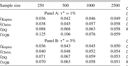
Table1 reports the size of tests forτ∗=1% and τ∗=5%. One can see that the asymptotic critical values do not do a good job whenτ∗=1% and the sample size is as small asT=250. In this case there are few observations around the 1% quan-tile ofRtimplying an inaccurate estimation ofQRt(0.01|Ft−1).
The VQR test responds to it by rejecting the null model more frequently than 5% of the time. However, we can see that if we allow for larger samples, the empirical size of the VQR test con-verges to its nominal size of 5%. It is important to mention that 1000 observations correspond to only four years of daily obser-vations, and therefore, it is a common sample size used in prac-tice by financial institutions. For instance, Berkowitz, Christof-fersen, and Pelletier (2009) used daily data ranging from 2001
Table 1. Empirical size of 5% tests
Sample size 250 500 1000 2500
Panel A:τ∗=1%
ζKupiec 0.036 0.042 0.046 0.049
ζChrist. 0.038 0.045 0.057 0.058
ζDQ 0.088 0.068 0.063 0.058
ζVQR 0.125 0.106 0.076 0.059
Panel B:τ∗=5%
ζKupiec 0.036 0.043 0.045 0.050
ζChrist. 0.040 0.048 0.052 0.054
ζDQ 0.071 0.067 0.059 0.053
ζVQR 0.070 0.063 0.058 0.051
to 2005 (about four years) to test VaR models used by different business lines of a financial institution.
The Kupiec and Christoffersen tests seem to be undersized when τ∗ =1% and the sample is as small as T =250, but their empirical size converges to the nominal size as the sam-ple increases. The same thing happens to the DQ test, which is slightly oversized for small samples but has correct size as the sample size increases. Whenτ∗=0.05, observations become more dense and consequently the quantiles are estimated more accurately. Since the 5% conditional quantile is now estimated more precisely, the improvement in the VQR test is relatively larger than in other tests. Indeed, whenτ∗=5% and sample is as small asT=250 the empirical size of the VQR and DQ tests are almost the same. As the sample increases, the empirical size of all tests converges to the nominal size of 5%. In sum, if the sample has a reasonable size then our theoretical findings are confirmed in the sense that all tests have correct size under the null hypothesis.
The main difference between the tests relates to their power to reject a misspecified model. To investigate power, we will assume that the correct data-generating process is again given by Equation (15). We must also choose a particular implemen-tation for the VaR calculation that is misspecified in that sense it differs from Equation (17). Following the industry practice (see Perignon and Smith2010), we assume that the bank uses a one-year historical simulation method to compute its VaR. Specifically,
Vt=percentile
{Rs}ts=t−Te,100τ
∗ . (18)
Historical simulation is by far the most popular VaR model used by commercial banks. Indeed, Perignon and Smith (2010) doc-umented that almost three-quarters of banks that disclose their VaR method report using historical simulation. Historical simu-lation is the empirical quantile, and therefore, does not respond well to increases in volatility (see Pritsker2001). Combining its popularity and this weakness it is the natural choice for the mis-specified VaR model (we note that Berkowitz, Christoffersen, and Pelletier2009used a similar experiment).
Table2reports the size-adjusted power. Whenτ∗=1% and the sample size is as small as 250, all tests present low power against the misspecified historical simulation model. Even in this situation, the VQR test is more powerful than any other test. When the sample size increases, the VQR test becomes
Table 2. Size-adjusted power of 5% tests
Sample size 250 500 1000 2500
Panel A:τ∗=1%
ζKupiec 0.059 0.113 0.189 0.322
ζChrist. 0.087 0.137 0.216 0.396
ζDQ 0.084 0.171 0.402 0.644
ζVQR 0.091 0.174 0.487 0.800
nzero 2.139 2.238 2.516 3.104
Panel B:τ∗=5%
ζKupiec 0.068 0.146 0.267 0.423
ζChrist. 0.142 0.227 0.319 0.509
ζDQ 0.179 0.316 0.454 0.769
ζVQR 0.215 0.366 0.644 0.883
nzero 2.521 3.033 3.960 6.946
even more powerful against the historical simulation model re-jecting such a misspecified model 17%, 49%, and 80% of the times when T=500, 1000, and 2500, respectively. This per-formance is by far the best one among all backtests considered in this article. The Kupiec test rejects the misspecified model only 32.2% of the times whenT=2500, which is close to the rate of the Christoffersen test (39.6%), but below the DQ test (64.4%). If a model is misspecified, then a backtest is supposed to use all available information to reject it. The Kupiec test has low power because it ignores the information about the time dependence of the hit process. The conditional coverage tests (Christoffersen and DQ) sacrifice information that comes from zero residuals, and therefore, fail to reject a misspecified model when the orthogonality condition holds, but the optimality con-dition does not. The VQR test simply compares the empirical conditional quantile that is estimated from the data with the conditional quantile estimated by using the historical simula-tion model. If these two estimates are very different from each other, then the null hypothesis is going to be rejected and the power of the test is delivered.
There are theoretically few observations below −Vt when τ∗=1%, which explains the low power exhibited by all tests. When τ∗ =5% the number of observations below −Vt
in-creases, giving to the tests more information that can be used to reject a misspecified model. Hence, we expect that the power of each test will increase when one considersτ∗=5% rather thanτ∗=1%. This additional information is used differently by each test. Here again the VQR benefits from using more in-formation than any other test to reject a misspecified model. Indeed, even for T =250 the VQR rejects the null hypothe-sis 21.5% of the times, above Kupiec (6.8%), Christoffersen (14.2%), and DQ (17.9%) tests. ForT=2500, the power of the VQR approaches 90% against 42.3%, 50.9%, and 76.9% for Kupiec, Christoffersen, and DQ, respectively.
Moreover, the reported differences in size-adjusted power can also be linked to the theoretical discussion in Section4.1. For instance, the main difference between the VQR and DQ tests is due to the nondifferentiability of the hit function when the error term is equal to zero. In this sense, we report in Ta-ble2the average number of times the error termutis actually
zero (so-callednzero). Recall from Section4.1thatnzerois
ex-pected to be at least equal to the dimension of β (i.e., in our casenzero≥2). Indeed, this result can be verified in Table2, in
which (in general) the more frequently the eventut=0 occurs,
the bigger the difference in size-adjusted power between the VQR and DQ tests. Also notice that as long as the sample size increases, the ratio nzero
T converges to zero, which gives support
to the assumption that this ratio isop(1)and that the DQ and
VQR are asymptotically equivalent.
Another advantage of the random coefficient framework pro-posed in this article is that it can be used to derive a statistical device that indicates why and when a given VaR model is mis-specified. In the next section we introduce this device and show how to use it to identify periods of risk exposure.
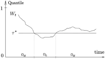
6. LOCAL ANALYSIS OF VAR MODELS: IDENTIFYING PERIODS OF RISK EXPOSURE
The conditional coverage literature is concerned with the ad-equacy of the VaR model in respect to the existence of clustered
violations. In this section, we will take an alternative route to analyze the conditional behavior of a VaR measure. According to Engle and Manganelli (2004), a good Value-at-Risk model should produce a sequence of unbiased and uncorrelated hits, and any noise introduced into the Value-at-Risk measure will change the conditional probability of a hit vis-à-vis the related VaR. Given that our study is entirely based on a quantile frame-work, besides the VQR test, we are also able to identify the ex-act periods in which the VaR produces an increased risk expo-sure in respect to its nominal levelτ∗, which is quite a novelty in the literature. To do so, let us first introduce some notation:
Definition 2. Wt ≡ {QUt(τ ) =τ ∈ [0,1] | −Vt =QRt(τ|
Ft−1)}, representing the empirical quantile of the standard iid uniform random variable, Ut, such that the equality −Vt = QRt(τ|Ft−1)holds at periodt.
In other words,Wt is obtained by comparingVt with a full
range of estimated conditional quantiles evaluated atτ∈ [0,1]. Note thatWtenables us to conduct a local analysis, whereas the
proposed VQR test is designed for a global evaluation based on the whole sample. It is worth mentioning that, based on our assumptions,QRt(τ|Ft−1)is monotone increasing inτ, andWt
by definition is equivalent to a quantile level, i.e.,Wt> τ∗⇔ QRt(Wt|Ft−1) >QRt(τ∗|Ft−1). Also note that if Vt is a
cor-rectly specified VaR model, thenWt should be as close as
pos-sible toτ∗ for allt. However, ifVt is misspecified, then it will
wander away fromτ∗, suggesting that−Vt does not correctly
approximate theτ∗th conditional quantile.
Notice that, due to the quantile regression setup, one does not need to know the true returns distribution to constructWt. In
practical terms, based on the seriesRt,Vtone can estimate the
conditional quantile functionsQRt(τ|Ft−1)for a (discrete) grid
of quantilesτ ∈ [0,1]. Then, one can constructWt by simply
comparing (in each time periodt) the VaR seriesVtwith the set
of estimated conditional quantile functionsQRt(τ|Ft−1)across
all quantilesτ inside the adopted grid.
Now consider the set of all observations=1, . . . ,T, in whichTis the sample size, and define the following partitions of:
Definition 3. L≡ {t∈|Wt< τ∗}, representing the
peri-ods in which the VaR is below the nominalτ∗level (indicating a conservative model).
Definition 4. H≡ {t∈|Wt≥τ∗}, representing the
peri-ods in which the VaR belongs to a quantile above the level of interestτ∗and thus underestimate the risk in comparison toτ∗. Since we partitioned the set of periods into two categories, i.e.,=H+L, we can now properly identify the so-called
periods of “risk exposure”H. Let us summarize the previous
concepts through the following schematic graph (Figure1). It should be mentioned that a VaR model that exhibits a good performance in the VQR test (i.e., in whichHois not rejected)
is expected to exhibitWt as close as possible toτ∗, fluctuating
aroundτ∗, in which periods ofWt belowτ∗ are balanced by
periods above this threshold. On the other hand, a VaR model rejected by the VQR test should present aWt series detached
fromτ∗, revealing the periods in which the model is conserv-ative or underestimate risk. This additional information can be extremely useful to improve the performance of the underlying Value-at-Risk model since the periods of risk exposure are now easily revealed.
Figure 1. Periods of risk exposure.
7. EMPIRICAL EXERCISE
7.1 Data
In this section, we explore the empirical relevance of the the-oretical results previously derived. This is done by evaluating and comparing two VaR models, based on the VQR test and other competing backtests commonly presented in the litera-ture. To do so, we investigate the daily returns of S&P500 over the last four years with an amount ofT=1000 observations, depicted in Figure2.
Note from the graph and the summary statistics the presence of common stylized facts about financial data (e.g., volatility clustering; mean reverting; skewed distribution; excess kurto-sis; and nonnormality, see Engle and Patton2001, for further details). The two Value-at-Risk models adopted in our eval-uation procedure are the popular 12-month historical simula-tions (HS12M) and the GARCH(1,1) model. According to Perignon and Smith (2010), about 75% of financial institu-tions in the U.S., Canada, and Europe that disclose their VaR model report using historical simulation methods. The choice of a GARCH(1,1)model with Gaussian innovations is motivated by the work of Berkowitz and O’Brien (2002), who documented that the performance of the GARCH(1,1) is highly accurate even as compared to more sophisticated structural models.
In addition, recall that we are testing the null hypothesis that the modelVt correctly approximates the true τ∗th conditional
quantile of the return seriesRt. We are not testing the null
hy-pothesis thatVt correctly approximates the entire distribution
ofRt. Therefore, it is possible that for differentτ’s (target
prob-abilities) the modelVtmight do well at a target probability, but
otherwise poorly (see Kuester, Mittik, and Paolella2005). Practice generally shows that different models lead to widely different VaR time series for the same considered return series,
leading us to the crucial issue of model comparison and hypoth-esis testing. The HS12M method has serious drawbacks and is expected to generate poor VaR measures since it ignores the dynamic ordering of observations and volatility measures look like “plateaus” due to the so-called “ghost effect.” On the other hand, as shown by Christoffersen, Hahn, and Inoue (2001), the GARCH-VaR model is the only VaR measure, among several alternatives considered by the authors, which passes Christof-fersen’s (1998) conditional coverage test.
7.2 Results
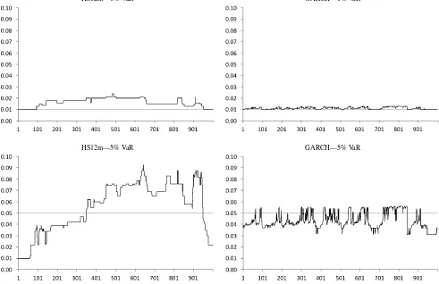
We start by showing the local analysis results for each VaR model. Whenτ∗=1, Figure3shows that the VaR computed by the HS12M method is above the 1% line most of the times, indi-cating that such a model over estimate 1% VaR very frequently. The same does not happen to the GARCH(1,1)model, which seems to yield VaR estimates that are very close to the 1% line. If we now turn our attention to the 5% Value-at-Risk, we can see that both models have a poor performance. Indeed, The VaR es-timated from the HS12M model seems to be quite erratic, with some periods in which 1% VaR is underestimated and other pe-riods in which it is overestimated. The GARCH(1,1) model seems to underestimate 5% VaR most of the times, although it does not seem to yield a VaR estimate that is far below 0.03. Therefore, if we backtest these two models we should expect to reject the 1% VaR estimated by HS12M and the 5% VaR estimated by HS12M and GARCH(1,1). The results from our backtesting are exhibited in Table3. Note that this local behav-ior investigation can only be conducted through our proposed quantile regression methodology, which we believe to be a nov-elty in the backtest literature.
Despite its poor local performance, the HS12M model is not rejected by Kupiec and Christoffersen tests at 5% level of sig-nificance. In part, this can explained by the fact that the Kupiec test is mainly concerned on the percentage of hits generated by the VaR model, which in the case of the HS12M model re-ported in Table3does not seem to be far away from the hypo-thetical levels. The null hypothesis of the Christoffersen test is very restrictive, being rejected when there is strong evidence of first order dependence of the hit function or when the percent-age of hits is far away fromτ∗. It is well known that there are many other forms of time dependence that are not accounted by the null hypothesis of the Christoffersen test. The more pow-erful test of Engle and Manganelli with the ex ante VaR as the
Figure 2. S&P500 daily returns (%).Notes: (a) The sample covers the period from 23/10/2003 until 12/10/2007; (b) Source: Yahoo!Finance.
HS12m—1% VaR GARCH—1% VaR
HS12m—5% VaR GARCH—5% VaR
Figure 3. Local analysis of VaR models.
only instrument performs quite well and rejects the misspecified HS12M model forτ∗=1% and 5%. As expected, the VQR test performs quite well, easily rejecting the misspecified HS12M.
In our local analysis, the GARCH(1,1) model seems to work well when we use it to estimate a 1% VaR, but fails to estimate a 5% VaR accurately. The backtest analysis in Table 3 indicates that neither test rejects the null hypothe-sis that the GARCH(1,1) is a correctly specified model for a 1% VaR. However, as documented by Kuester, Mittik, and Paolella (2005), it is possible that for different τ∗’s (target probabilities) the model can do well at a given target proba-bility, but otherwise poorly at another target probability. Here, the GARCH(1,1) model seems to predict the 1% VaR quite well but not the 5% VaR. However, when we backtest the GARCH(1,1)forτ∗=5% by using the existing backtests, we fail to reject the null hypothesis. These results suggest that the GARCH(1,1)model correctly predicts the 5% VaR despite the
Table 3. Backtesting Value-at-Risk models
Model % of hits ζKupiec ζChrist. ζDQ ζVQR
τ∗=1%
HS12M 1.6 0.080 0.110 0.000 0.000
GARCH(1,1) 1.1 0.749 0.841 0.185 0.100
τ∗=5%
HS12M 5.5 0.466 0.084 0.000 0.000
GARCH(1,1) 4.5 0.470 0.615 0.841 0.042
NOTE: p-values are shown in theζ’s columns.
clear evidence against it showed in Figure3. The results of Ta-ble3indicate that GARCH(1,1)model for the 5% VaR is only rejected by the VQR test, which is compatible with the previ-ous evidence in Figure3. Our methodology is, therefore, able to reject more misspecified VaR models in comparison to other backtests.
8. CONCLUSIONS
Backtesting can prove very helpful in assessing Value-at-Risk models and is nowadays a key component for both regula-tors and risk managers. Since the first procedures suggested by Kupiec (1995) and Christoffersen (1998), a lot of research has been done in the search for adequate methodologies to assess and help improve the performance of VaRs, which (preferably) do not require the knowledge of the underlying model.
As noted by the Basel Committee (1996), the magnitude as well as the number of exceptions of a VaR model is a matter of concern. The so-called “conditional coverage” tests indirectly investigate the VaR accuracy, based on a “filtering” of a seri-ally correlated and heteroscedastic time series (Rt) into a
seri-ally independent sequence of indicator functions (hit sequence
Hitt). Thus, the standard procedure in the literature is to verify
whether the hit sequence is iid. However, an important piece of information might be lost in that process since the condi-tional distribution of returns is dynamically updated. This issue is also discussed by Campbell (2005), who stated that the re-ported quantile provides a quantitative and continuous measure
of the magnitude of realized profits and losses, while the hit indicator only signals whether a particular threshold was ex-ceeded. In this sense, the author suggested that quantile tests can provide additional power to detect an inaccurate risk model. That is exactly the objective of this article: to provide a VaR-backtest fully based on a quantile regression framework. Our proposed methodology enables us to: (i) formally conduct a Wald-type hypothesis test to evaluate the performance of VaRs and (ii) identify periods of an increased risk exposure. We illus-trate the usefulness of our setup through an empirical exercise with daily S&P500 returns in which we construct two compet-ing VaR models and evaluate them through our proposed back-test (and through other standard backback-tests).
Since a Value-at-Risk model is implicitly defined as a condi-tional quantile function, the quantile approach provides a nat-ural environment to study and investigate VaRs. One of the ad-vantages of our approach is the increased power of the sug-gested quantile-regression backtest in comparison to some es-tablished backtests in the literature, as suggested by a Monte Carlo simulation. Perhaps most importantly, our backtest is ap-plicable under a wide variety of structures since it does not de-pend on the underlying VaR model, covering either case where the VaR comes from a conditional volatility model or it is di-rectly constructed (e.g., CAViaR or ARCH quantile methods) without relying on a conditional volatility model. We also in-troduce a main innovation. Based on the quantile estimation, one can also identify periods in which the VaR model might increase the risk exposure, which is a key issue to improve the risk model, and probably a novelty in the literature. A final ad-vantage is that our approach can easily be computed through standard quantile regression software.
Although the proposed methodology has several appealing properties, it should be viewed as complementary rather than competing with the existing approaches due to the limitations of the quantile regression technique discussed in this article. Furthermore, several important topics remain for future re-search, such as: (i) time aggregation—how to compute and properly evaluate a 10-day regulatory VaR? Risk models con-structed through quantile autoregressive (QAR) technique can be quite promising due to the possibility of recursively gen-eration of multiperiod density forecast (see Koenker and Xiao 2006a,2006b); (ii) our randomness approach of VaR also de-serves an extended treatment and leaves room for weaker con-ditions; (iii) multivariate VaR—although the extension of the analysis for the multivariate quantile regression is not straight-forward, several proposals were already suggested in the liter-ature (see Chaudhuri1996and Laine2001); (iv) inclusion of other variables to increase the power of VQR test in other di-rections; (v) improvement of the Basel formula for market re-quired capital; and (vi) nonlinear quantile regressions; among many others.
According to the Basel Committee (2006), new approaches to backtesting are still being developed and discussed within the broader risk management community. At present, differ-ent banks perform differdiffer-ent types of backtesting comparisons and the standards of interpretation also differ somewhat across banks. Active efforts to improve and refine the methods cur-rently in use are underway, with the goal of distinguishing more sharply between accurate and inaccurate risk models. We aim
to contribute to the current debate by providing a quantile tech-nique that can be useful as a valuable diagnostic tool as well as a means to search for possible model improvements.
APPENDIX A: PROOFS OF PROPOSITIONS
Proof of Proposition1
Given the random coefficient model in Equation (2), we can compute the conditional quantile of Rt asQRt(τ|Ft−1)= Q[α0(Ut)+α1(Ut)Vt](τ|Ft−1). Comonotonicity implies that Qp
i=1αi(Ut)= p
i=1Qαi(Ut). Therefore, we can write QRt(τ|
Ft−1)=Qα0(Ut)(τ|Ft−1)+Qα1(Ut)Vt(τ|Ft−1). Sinceαi(Ut)are
increasing functions of the iid standard uniform random vari-able Ut, then we know thatQαi(Ut)=αi(QUt), and therefore, QRt(τ|Ft−1)=α0(QUt(τ ))+α1(QUt(τ ))Vt. Finally, recall that Ut∼iid U(0,1), and therefore,QUt(τ )=τ,τ ∈(0,1), which
impliesQRt(τ|Ft−1)=α0(τ )+α1(τ )Vt,τ ∈(0,1).
Proof of Proposition2
By Assumption1, together with comonotonicity ofαi(Ut), i =0,1, we have that the conditional quantile function is monotone increasing inτ, which is a crucial property of Value-at-Risk models. In other words, we have that QRt(τ1|Ft−1) < QRt(τ2|Ft−1)for allτ1< τ2∈(0,1). Assumptions2through4
are regularity conditions necessary to define the asymptotic co-variance matrix and a continuous conditional quantile func-tion, needed for the CLT (6) of Koenker (2005, theorem 4.1). A sketch of the proof of this CLT, via a Bahadur representa-tion, is also presented in Hendricks and Koenker (1992, appen-dix). Given that we established the conditions for the CLT (6), our proof is concluded by using standard results on quadratic forms: For a given random variablez∼N(μ, )it follows that
(z−μ)′−1(z−μ)∼χr2, wherer=rank(). See Johnson and Kotz (1970, p. 150) and White (1984, theorem 4.31) for further details.
ACKNOWLEDGMENTS
The authors thank the joint editor Arthur Lewbel, an anony-mous associate editor, two anonyanony-mous referees, and Igna-cio Lobato, Richard Smith, Juan Carlos Escanciano, and Keith Knight for their helpful comments and suggestions. Gaglianone gratefully acknowledges financial support from CAPES (scholarship BEX1142/06-2) and Programme Alban (grant E06D100111BR). Lima thanks CNPq for financial sup-port as well as the University of Illinois. Linton thanks the ESRC and Leverhulme foundations for financial support as well as the Universidad Carlos III de Madrid-Banco Santander Chair of Excellence. Daniel Smith thanks the Social Sciences and Humanities Research Council of Canada for financial sup-port. The opinions expressed in this article are those of the au-thors and do not necessarily reflect those of the Central Bank of Brazil. Any remaining errors are ours.
[Received December 2007. Revised May 2009.]
REFERENCES
Basel Committee on Banking Supervision (1996), “Amendment to the Capital Accord to Incorporate Market Risks,” technical paper, BIS—Bank of Inter-national Settlements. [158]
(2006), “International Convergence of Capital Measurement and Cap-ital Standards,” technical paper, BIS—Bank of International Settlements. [159]
Berkowitz, J., and O’Brien, J. (2002), “How Accurate Are the Value-at-Risk Models at Commercial Banks?”Journal of Finance, 57, 1093–1111. [152, 157]
Berkowitz, J., Christoffersen, P., and Pelletier, D. (2009), “Evaluating Value-at-Risk Models With Desk-Level Data,”Management Science, 1–15. Pub-lished online ahead of print January 28, 2009. [151,153-155]
Buchinsky, M. (1998), “Recent Advances in Quantily Regression Models: A Practical Guideline for Empirical Research,”The Journal of Human Re-sources, 33, 88–126. [154]
Campbell, S. D. (2005), “A Review of Backtesting and Backtesting Proce-dures,” Finance and Economics Discussion Series Working Paper 21, Fed-eral Reserve Board, Washington, DC. [158]
Chaudhuri, P. (1996), “On a Geometric Notion of Quantiles for Multivariate Data,”Journal of the American Statistical Association, 91, 862–872. [159] Christoffersen, P. F. (1998), “Evaluating Interval Forecasts,”International
Eco-nomic Review, 39, 841–862. [150,153,154,157,158]
Christoffersen, P. F., and Goncalves, S. (2005), “Estimation Risk in Financial Risk Management,”Journal of Risk, 7, 1–28. [153]
Christoffersen, P. F., and Pelletier, D. (2004), “Backtesting Value-at-Risk: A Duration-Based Approach,”Journal of Financial Econometrics, 2 (1), 84–108. [154]
Christoffersen, P. F., Hahn, J., and Inoue, A. (2001), “Testing and Comparing Value-at-Risk Measures,”Journal of Empirical Finance, 8, 325–342. [151, 157]
Daníelsson, J., Jorgensen, B. N., Samorodnitsky, G., Sarma, M., and de Vries, C. G. (2005), “Subadditivity Re-Examined: The Case for Value-at-Risk,” manuscript, London School of Economics. Available at www. RiskResearch.org. [150]
Dufour, J.-M. (2006), “Monte Carlo Tests With Nuisance Parameters: A Gen-eral Approach to Finite-Sample Inference and Nonstandard Asymptotics in Econometrics,”Journal of Econometrics, 133, 443–477. [154]
Engle, R. F., and Manganelli, S. (2004), “CAViaR: Conditional Autoregressive Value at Risk by Regression Quantiles,”Journal of Business & Economic Statistics, 22 (4), 367–381. [150,153,154,156]
Engle, R. F., and Patton, A. J. (2001), “What Good Is a Volatility Model?”
Quantitative Finance, 1, 237–245. [151,157]
Giacomini, R., and Komunjer, I. (2005), “Evaluation and Combination of Con-ditional Quantile Forecasts,”Journal of Business & Economic Statistics, 23 (4), 416–431. [150]
Haas, M. (2005), “Improved Duration-Based Backtesting of Value-at-Risk,”
Journal of Risk, 8 (2), 17–38. [154]
Hartz, C., Mittnik, S., and Paolella, M. (2006), “Accurate Value-at-Risk Fore-casting Based on the Normal-GARCH Model,”Computational Statistics & Data Analysis, 51 (4), 2295–2312. [153]
Hendricks, W., and Koenker, R. (1992), “Hierarchical Spline Models for Con-ditional Quantiles and the Demand for Electricity,”Journal of the American Statistical Association, 87 (417), 58–68. [152,159]
Huber, P. J. (1967), “The Behavior of Maximum Likelihood Estimates Under Nonstandard Conditions,” inProceedings of the 5th Berkeley Symposium on Mathematical Statistics and Probability, Vol. 4, Berkeley, CA: University of California Press, pp. 221–233. [152]
Ibragimov, R., and Walden, J. (2007), “Value at Risk Under Dependence and Heavy-Tailedness: Models With Common Shocks,” manuscript, Harvard University. [150]
Issler, J. V., and Lima, L. R. (2009), “A Panel Data Approach to Economic Forecasting: The Bias-Corrected Average Forecast,”Journal of Economet-rics, 152 (2), 153–164. [151]
Johnson, N. L., and Kotz, S. (1970),Distributions in Statistics: Continuous Univariate Distributions, New York: Wiley Interscience. [159]
Koenker, R. (2005),Quantile Regression, Cambridge: Cambridge University Press. [152,154,159]
Koenker, R., and Machado, J. A. F. (1999), “Goodness of Fit and Related Infer-ence Processes for Quantile Regression,”Journal of the American Statisti-cal Association, 94 (448), 1296–1310. [152]
Koenker, R., and Xiao, Z. (2002), “Inference on the Quantile Regression Process,”Econometrica, 70 (4), 1583–1612. [150,152]
(2006a), “Quantile Autoregression,”Journal of the American Statisti-cal Association, 101 (475), 980–990. [159]
(2006b), Rejoinder to “Quantile Autoregression,” Journal of the American Statistical Association, 101 (475), 1002–1006. [159]
Koenker, R., and Zhao, Q. (1996), “Conditional Quantile Estimation and Infer-ence for ARCH Models,”Econometric Theory, 12, 793–813. [152] Kuester, K., Mittik, S., and Paolella, M. S. (2005), “Value-at-Risk Prediction:
A Comparison of Alternative Strategies,”Journal of Financial Economet-rics, 4 (1), 53–89. [157,158]
Kupiec, P. (1995), “Techniques for Verifying the Accuracy of Risk Measure-ment Models,”Journal of Derivatives, 3, 73–84. [150,153,154,158] Laine, B. (2001), “Depth Contours as Multivariate Quantiles: A Directional
Approach,” Master’s thesis, Université Libre de Bruxelles. [159]
Mincer, J., and Zarnowitz, V. (1969), “The Evaluation of Economic Forecasts and Expections,” inEconomic Forecasts and Expections, ed. J. Mincer, New York: National Bureau of Economic Research. [152]
Morgan, J. P. (1996),RiskMetrics—Technical Document(4th ed.), New York: Morgan Guaranty Trust Company of New York. [150]
Newey, W. K., and McFadden, D. (1994), “Large Sample Estimation and Hy-pothesis Testing,” inHandbook of Econometrics, Vol. 4, Amsterdam: Else-vier B.V. North-Holland, Chapter 36, pp. 2111–2245. [154]
Parzen, M. I., Wei, L., and Ying, Z. (1994), “A Resampling Method Based on Pivotal Estimating Functions,”Biometrika, 81, 341–350. [154]
Pascual, L., Romo, J., and Ruiz, E. (2006), “Bootstrap Prediction for Re-turns and Volatilities in GARCH Models,”Computational Statistics & Data Analysis, 50, 2293–2312. [153]
Perignon, C., and Smith, D. (2010), “The Level and Quality of Value-at-Risk Disclosure by Commercial Banks,”Journal of Banking and Finance, 34, 362–377. [155,157]
Pritsker, M. (2001), “The Hidden Dangers of Historical Simulation,” Finance and Economics Discussion Series 27, Board of Governors of the Federal Reserve System, Washington. [155]
Powell, J. L. (1984). “Least Absolute Deviations Estimation for the Censored Regression Model,”Journal of Econometrics, 25, 303–325. [154] Robinson, P. M. (2006), Comment on “Quantile Autoregression,” by
R. Koenker and Z. Xiao,Journal of the American Statistical Association, 101 (475), 1001–1002. [152]
White, H. (1984),Asymptotic Theory for Econometricians, San Diego: Acad-emic Press. [159]
Wu, G., and Xiao, Z. (2002), “An Analysis of Risk Measures,”Journal of Risk, 4, 53–75. [152]