11 (2000) 255 – 293
Modeling industrial dynamics with innovative
entrants
S.G. Winter
a, Y.M. Kaniovski
b,c, G. Dosi
d,*
aThe Wharton School,Uni6ersity of Pennsyl6ania,2000Steinberg Hall-Dietrich Hall,Philadelphia,
PA19104.6370,USA
bThe International Institute for Applied Systems Analysis,A-2361Laxenburg,Austria cUni6ersity of Trento,Via Inama5,I-38100Trento,Italy
dThe Sant’Anna School of Ad6anced Studies,Via Carducci40,I-56127Pisa,Italy
Accepted 22 June 1999
Abstract
The paper analyzes some generic features of industrial dynamics whereby innovative change is carried, stochastically, by new entrants. Relying on the formal representation suggested in Winter, S.G., Kaniovski, Y.M., Dosi, G., 1997. A Baseline Model of Industry Evolution. [Interim Report IR-97-013/March, International Institute for Applied Systems Analysis, Laxenburg, Austria], it studies both the asymptotic properties of such processes and their appropriability to account for a few empirical stylized facts, including persistent entry and exit, skewed size distributions and turbulence in market shares. © 2000 Elsevier Science B.V. All rights reserved.
Keywords:Evolution; Competition; Learning; Stochastic entry; Entrepreneurial startups; Expanding set of technological opportunities; Industrial dynamics
www.elsevier.nl/locate/econbase
1. Introduction
In this work we explore the dynamic features of industries characterized by the persistent arrival of innovative entrants. The models which follow build upon and modify the baseline model presented in Winter et al. (1997). In an extreme synthesis, in the latter we develop a framework of analysis of the competitive
* Corresponding author.
E-mail address:[email protected] (G. Dosi).
dynamics of industries composed of heterogeneous firms and continuing stochastic entry. There, we show that despite the simplicity of the assumptions, the model is able to account for a rather rich set of empirical ‘stylized facts’, such as: (i) continuing turbulence in market shares; (ii) persistent inflows and outflows of firms; (iii) ‘life cycle’ phenomena — including, in particular, nearer the birth of an industry, relatively sudden ‘shakeouts’, yielding distinctly different industrial struc-ture thereafter; and (iv) skewed size distributions of firms1
.
The ‘heroic’ simplicity of Winter et al. (1997) goes as far as assuming that the set of technological options among which entrants draw — as a formal metaphor of their diverse capabilities — is given from the start and is invariant throughout the unfolding evolution of the industry. While this assumption is certainly in tune with the spirit of most evolutionary game-theoretical set-ups, it is also at odds with an overwhelming empirical evidence highlighting the role of innovators as carriers of technological and organizational discoveries. Typically, these discoveries happen to be tapped at some point in the history of an industry on the grounds of the available knowledge base at that time, but would not have been possible earlier on, given the knowledge base at that earlier time.
More formally, this implies that what is commonly called the ‘production possibility set’ endogenously shifts, due to the cumulative (but stochastic) effects of exploration by potential innovators2
.
The model which follows studies the properties of industrial dynamics which correspond to that archetype of industrial evolution which some authors call
Schumpeter Mark Iregime (cf. Dosi et al., 1995; Malerba and Orsenigo, 1995). In
short, while of course both incumbents and new entrants empirically attempt to explore — to varying degrees — yet unexploited opportunities of innovation, here we focus upon the properties of that extreme archetype whereby only entrants have a positive probability of advancing the current state of technological knowledge. (Hence the name of such a ‘regime’, in analogy with the emphasis of Schumpeter (1934) upon novel entrepreneurial efforts as drivers of change.)
Compared with the cited ‘baseline model’ discussed in Winter et al. (1997), in the following we shall try to disentangle those properties which appear to be generic features of a wide class of processes of industrial dynamics simply resting upon persistently heterogeneous agents and market selection and, conversely, those properties which depend upon more specific forms of innovative learning, such as
theSchumpeter Mark Iregime considered here3. As we shall show below, some of
the emerging ‘stylized facts’ of the modeled dynamics appear to robustly hold in
1This evidence is discussed at much greater length in the special issues ofIndustrial and Corporate
Change, 5, 1997 and ofThe International Journal of Industrial Organization, 4, 1995. See also Baldwin (1995); Carroll and Hannan (1995); Davis et al. (1996); Dunne et al. (1988); Dosi et al. (1995); Geroski (1995); Hannan and Freeman (1989).
2For more detailed empirical corroborations of these points, cf., among others, Dosi (1988) and
Freeman and Soete (1997).
3See Winter et al. (1997) also for some comparative assessment of somewhat germane models of
both set-ups, with or without innovative entry. Other features, including some path-dependence properties, interestingly, appear only when ‘open-ended’ dynamics on technological opportunities is accounted for, as we do in this work.
Section 2 sets out the basic structure of the model, in a first specification with innovative learning by entrants directed at increasing capital productivity, and, conversely, in Section 3, we study the properties of a symmetrical assumption of (stochastically) increasing labour efficiencies.
2. The basic framework of the model: a first setting with increasing capital efficiencies
Let us assume an industry evolving in discrete timet=0, 1, …. Att=0 there are no firms ready to produce, but k firms arrive to the industry, ready to start manufacturing att=1. Techniques are capital-embodied and firm-specific. So, the model which follows can be interpreted as a vintage capital model, with heteroge-neous techniques across firms also within each vintage.
At timet]1 the industry consists of nt firms which are involved in production
and a number of new firms that enter at t and will participate in manufacturing from t+1 onward. Uniformly for the whole industry we have:
6 — price per unit of physical capital, 6\0,
d — depreciation rate of the capital stock, 0Bd51.
In the first version of the model which follows the output is produced by capital alone. The competitiveness of any firm represented in the industry is ultimately determined by its capital per unit of output. Let us designate the latter byaifor the
i-th firm. As time goes on, the ‘best’ capital/output ratio (in real terms) attainable in the industry stochastically decreases.
Let us further assume the following endogenous stochastic mechanism of learning by entrants. Take a random variablejwith positive mean jand a finite variance Dj. Set z for a random variable distributed over [a, b], 0BaBbB . For each time instantt]0 we allow for the industry to havek]1 new firms whose levels of capital per unit of output are randomly determined as exp{−At}zi, tk+15i5
(t+1)k. Here At+1=At+jt+1, t]0, A0=j0 Also, jt, t]0, and ji, i]1, are
mutually independent collections of realizations ofj andz. Thus, all capital ratios feasible for newcomers at time t belong to [exp{−At}a, exp{−At}b]. Their
distribution within this interval is governed by a realization of exp{−At}z.
Consequently, At characterizes in a probabilistic way the highest productivity of
capital attainable to newcomers in the industry at timet. Note that by construction
in this competiti6e en6ironment only newcomers learn to impro6e the producti6ity of
capital.
It is important to notice that the assumption of a fixed number of entrants is just made here for expositional simplicity. The qualitative results do not change if one
allows stochastic entry (as we in fact do in Winter et al., 1997) and if entry probabilities were made dependent upon some state variable of the system, for example, the current level of profitability in the industry: see Remark 2.2. below.
The productive capacity of thei-th firm is Qt i=K
i(t)/ai, where Ki(t) stands for
the capital of thei-th firm at time t. The total productive capacity of the industry involved in manufacturing at time tis
Qt=%
nt
i=1
Qt i.
We assume a decreasing continuous demand functionp=H(q), mapping [0,) in [0,H(0)] such that H(0)B and H(q)0 as q , where as usual, p stands for the price and q for demanded quantities. [Thus, the price at time t equals H(Qt).] The gross profit per unit of output at tis alsoH(Qt) since, without loss of
generality we may also assume zero variable costs. The gross investment per unit of output attis a share of the gross profit, i.e. lH(Qt), where the constantlcaptures
the share of the gross profit which does not leak out as the interest payments and shareholders’ dividends, and can be considered to be a measure for the propensity to invest. The total gross investment per unit of capital for the i-th firm at timet readslH(Qt)/6ai.
For each capital ratio generated at t we shall allow a single entrant. Entrants’ initial capitals are independent realizations ui,
i]1, of a random variable u
distributed over [c,h], 0BcBhB . (It is assumed that the realizations ofj,zand u are mutually independent random variables.)
To complete the description of the competitive environment we need some death mechanism. A firm is dead at time t and does not participate in the production process fromt+1 onward if its capital at t is less than oc, o(0, 1]4
We assume that all random elements are given on a probability space {V,F,P}. In order to study the long run behavior of this industry, let us give a formal description of its evolution.
2.1.A dynamical setting of the model
Let firmibe manufacturing during timet. Our investment rule implies that at the end of this production period its capital is
Qt i
ai
1−d+l
6a
i
H(Qt)
n
.If this value does not drop below the death threshold oc, the firm continues to manufacture during time instantt+1. Otherwise it dies. To capture these possibil-ities, we introduce
4The situation without mortality can be thought of as a limit case when o=0. Conversely, for a
x
Qti
1−d+l
6aiH
(Qt)
n
]oc/aithe indicator function of the event that the firm continues to manufacture. As usual, for a relation Awe set that
xA={1, if A is true, 0, otherwise.
Now the evolution of the i-th firm (in terms of productive capacity) reads
Qti+1=Qti
1−d+l
6ai
H(Qt)
n
xQti
1−d+ l6ai
H(Qt)
n
]oc/ai. (2.1)These equations are not handy for analysis. Mortality implies thatnt, the number
of firms in business, changes over time. Thus, we have a system with a variable dimension. Moreover, these equations do not incorporate the entry process: hence Eq. (2.1) only captures a part of the evolution of the industry. In order to handle entry and variable numbers of incumbents one needs a dynamic representation of the model that leaves room for all feasible development paths. It is nested in an infinite dimensional space.
The intuition is the following. Even if at each time one assumes, quite naturally, a finite number of entrants, as time goes to infinity, one must allow for an infinite number of firms to visit the industry. Moreover, the number of firms is normally changing over time as the joint outcome of entry and selection (entailing mortality). Somewhat similar considerations apply to the input coefficients (i.e. the productiv-ities) which the system explores. The rather novel formal machinery developed below is precisely aimed to rigorously capture these properties.
Introduce a space R of vectors with denumerably many coordinates. Set
R=R
i=1
Ri
n
,where stands for the direct sum of a real lineRand 2k-dimensional real vector spaces Ri, i]1. Thus, for every qR
q=q
i=1q
i
n
(2.2)withqR and qiR
i, i]1. Define an automorphism D(·) on R such that
D(q)=D1(
q)
i=2D
i(
q)
n
,whereD1(·):R
RR1R2 and Di(·):RRi, i]3. Let
D1
1
(q)=q, Ds
1
(q)=0, 25s52k+1, D2k+j+1 1
(q)=qj
1
exp{−q}xA j 1(q),
D3k+j+1
1 (
qk+j
1
1−d+l
6H
%k s=1
qk+s1 exp{
q}/qs
1 +%
i=2
qk+s i
/qs i
n
exp{q}/qj
1
n
xAj 1(q);
Dji(q)=qjixA j i(q),
Dki+j(q)=qki+j
1−d+l
6H
%k s=1
qk1+sexp{q}/qs1+ %
p=2
qkp+s/qps
n
,
qjin
xA j i(q),where 15j5k,i]2, Aj1(
q) designates the relation
qk1+j
1−d+l
6H
%k s=1
qk1+sexp{q}/qs1+%
i=2
qki+s/qsi
n
exp{q}/qj1n
]ocandAji(
q) stands for the relation
qki+j
1−d+l
6H
%k s=1
qk1+sexp{q}/qs1+ %
p=2
qkp+s/qsi
n
,
qjin
]oc.We restrict ourselves to vectorsq defined by Eq. (2.2) belonging to
R
+=[0,)
i=1
R+i
n
and set H()=0 for the case when the iterated sum involved in the above expressions is infinite. Here
R+i ={qiRi: qji\0,qki+j]0,j=1, 2, …,k}, i]1.
Also,Ds
i(·) and q s
i stand for the s-th coordinates of
Di(·) and
qi.
Define infinite dimensional random vectors Yt, t]0, setting
Y1t=jt, Yti+1=ztk+i, Ytk+i+1=utk+i, i=1, 2, …,k, Yjt=0
j]2k+2.
(Note that here we number coordinates linearly rather than in terms of cohorts as above.)
The evolution of the industry is as follows
q(t+1)=D(q(t))+Yt+1
, t]0, q(0)=Y0
, (2.3)
Since Yt are independent in t, this expression defines a Markov process on R
+.
Moreover, since the deterministic operatorD(·) as well as the distribution of Yt do
not depend on time, the process is homogeneous in time.
Conceptually, this phase space is formed by the value characterizing the highest productivity which is potentially attainable at any time in the industry (the first coordinate), capitals per unit of output (the firstkcoordinates in each cohort, that is, a 2k box in the above structure) and individual capital stocks (the last k coordinates in each cohort: that is, to a capital ratio placed at the j-th position corresponds the capital placed at the (k+j)-th position) of all firms that stay alive. Therefore, ifqk+i
n (
t)\0 for somei=1, 2, …,kandn5t, then a firm withqi n(
period. The representation via a direct sum seems to be a handy way of explicitly capturing the dynamic of cohorts.
The formulas for Di(·), i
]2, reflect our investment rule together with the
assumption that the capital ratio remains constant through the life time of a firm. In analogy with Eq. (2.1), they are capturing the dynamic of capital stocks (but more precisely Eq. (2.1) refers to productive capacities). The indicators are needed because of the death rule5. The relation A
j
i(q) gives the criterion that a firm from
thei-th box placed at thej-th position continues to manufacture given the state of the industryq. As from above, the first coordinate carries the value determining the highest productivity attainable in the industry. The further 2kblock is zero to host newcoming firms. The next k ones reflect the learning rule on improvement of productivity adopted by newcoming firms. Finally, the lastk coordinates of D1
(·) are defined according to our investment rule.
Given this formal description of this process of industry evolution, let us proceed to the analysis of its long run behavior.
2.2.Asymptotic properties of the industry
Define B
the minimal s-field in R generated by sets of the following form
A=A
j=1A
j
n
, (2.4)
whereAdesignates a set from the s-field of Borel sets B on the real line, andAj
being a set from thes-field of Borel sets Bj in Rj. For every such set Aone step
transition probability of process Eq. (2.3) reads
p1
(q,A)=P{D(q)+YA}=P{Y*AA1}xD(q)
i=2
Ai (2.5)
HereY* stands for the (2k+1)-dimensional vector whose coordinates coincide with first 2k+1 coordinates of a generic vector Y having the same distribution as Yt,
t]0.
To study the ergodic properties of process (2.3), we need the following condition which is due to Doeblin (see Doob, 1953, p. 192).
There is a finite positive measuref(·) withf(R
+)\0 and a positive numberd
such that for allqR
+p1(q, A)51−d if f(A)5d.
For a setAas in (2.4) letf(A)=P{Y*AA1}. From (2.4) it follow thatp1(q,
A)5f(A). Sincef(R
+)=P{Y*[0,)R 1
+}=1, restricting ourselves tod51/
2, we get that, if f(A)5d then p1(q, A)5d51−d. Thus, Doeblin’s condition
holds for this choice of f(·) and all d(0, 1/2].
Now, by Theorem 5.7 from Doob (1953) (p. 214), we see that
5In particular, applied to the first kcoordinates in a cohort, they prevent from carrying over the
p(q,A)= lim
n 1
n %
n t=1
pt(
q,A)
defines for each qR
+ a stationary absolute distribution. Herept(x, ·) stands for
the transition probability in tsteps, that is,
pt(q,A)=
&
R+
pt−1(y,A) dp1(q,y), t]2.
The stationary distributionp(q, ·) turns out to be the same, that is p£(·) for all q
belonging to the same ergodic set £ (see Doob, 1953, p. 210). It has the following generic property
&
£
p1(
x,A) dp£(x)=p£(A).
In general, it is not possible to find an explicit expression for p£(·) from this relation.
Thus, we may only obtain the following result concerning ergodicity of process Eq. (2.3).
Theorem 2.1. For e6ery setA gi6en by Eq. (2.4) with probability one 1
n %
n t=1
pt
(Y0
,A)p(Y0
,A) (2.6)
as n . Herep(Y0, ·)is a stochastic probability measure(since it depends on Y0),
withp£(·) for any elementary outcomevV whereby Y0 belongs for this elementary
outcome to an ergodic set £.
Consider the implications of this result in terms ofpath dependency. On the one hand, Doeblin’s condition implies that events occuring at t and t+n are getting more and more statistically independent as n increases. Thus, the impact of the initial state vanishes as time goes on. Should one be able to prove that there is a single ergodic set, then the limit of time averages in Eq. (2.6) would not depend on the initial state, and hence the lack of path-dependency. On the other hand, the limit in Eq. (2.6), in general, does depend on the initial state. But the dependency acts in a way that such limit turns out to be the same for all initial states belonging to the same ergodic set. Therefore, there might indeed be some path-dependency which is governed by a partition of V. Note also that this partition, in general,
turns out to be less fine than the one given by Y0.
rt=
QtH(Qt)
%
i=1 %k
j=1
qk+j i (t)
for the gross profit rate att]1. Since there is no production at t=0,r0=0. As a
consequence of Theorem 2.1 we have the following statement.
Corrollary 2.1.If xH(x)5const for x , then with probability one
1
n %
n i=1
ri
&
R+
Q(y)H(Q(y))
%
i=1 %
k j=1
yki+j
dp(Y0, dy) (2.7)
as n . Here for a vectory of the form Eq. (2.2)
Q(y)= %
k s=1
yk+s1 exp{
y}/ys
1 +%
i=2
yk+s i
/ys i
n
.Indeed,QtH(Qt)5const by hypothesis. Also
%
i=1 %
k s=1
qki+j(t)] % k i=1
u(t−1)k+i]kc, t]1.
Hence rt5const/kcB . Which implies that Eq. (2.7) follows from Eq. (2.6).
Note that if limx xH(x)=H, then
1
n %
n i=1
riH
&
R+
dp(Y0, y)
%
i=1 %
k j=1
yk+j i
.
As mentioned, the total productive capacity of this industry unboundedly in-creases as time goes on. More precisely, we have the following statement.
Lemma 2.1. The total producti6e capacity Qt of the industry goes to infinity with
probability one as t .
The lemma is proved in the Appendix.
Now let us study the mortality of firms in this competitive environment.
Theorem 2.2.If o\0, then e6ery firm dies in a finite random time with probability one.
Having shown the unbounded increase of productive capacity as time goes on, let us now characterize its rate of growth.
Theorem 2.3. With probability one exp{−at}Qt as t for e6ery aBEj.
Moreo6er, if
lim
x
H(x)x=0, (2.8)
then with probability one exp{−at}Qt0 as t for e6erya\Ej.
The theorem is proved in the Appendix.
Remark 2.1. The same result obtains if, instead of Eq. (2.8), we require that
lim sup
x
H(x)xBdk6ca
lb . (2.9)
Now, if for a positive number H a demand function decreases as H/x forx ,
then, keeping all other parameters of the model involved in the right hand side of Eq. (2.9) fixed, one can ensure Eq. (2.9) just increasingk. Thus, for such demand functions the second statement of Theorem 2.3 always holds true if the number of newcoming firms is large enough.
We have showed that the productive capacity of the industry always grows faster than exp{ta} for everyaBEj. If, additionally, the demand function declines fast enough (see Eq. (2.8) or Eq. (2.9)), then the productive capacity always grows slower than exp{ta} for every ora\Ej. Consequently,the threshold6alue Ejis the
only candidate for the growth rate in the class of exponential functions of time. This
growth is entirely due to the increasing efficiency of newcoming firms, and is not dependent upon the investment mechanism employed in the model. Interestingly, one is not able to prove that exp{−tEj}Qt converges to a limit as t increases.
Indeed, here we are facing with a 6ariety of growth regimes. Each of them is determined probabilistically by the development path (i.e. also a particular ‘techno-logical trajectory’) and is deviating from the main trend, exp{tEj}, by a value vanishing ast faster than exp{−tb} for every b\0. Hence, these de6iations
are not detectable if we restrict oursel6es to the class of exponential functions
of time. To understand why this happens, let us consider the asymptotic behavior
of the value Vt giving the lower bound for the total productive capacity since
Qt+1]Vt.
The random variableVtis a product of the two other ones: exp{At} andUt. The
latter, Ut does not contribute to the growth rate since its distribution does not
depend ont, being a convolution ofkcopies ofu/z. Hence, let us focus onAt. We
have that
At=%
t i=0
ji
=(t+1)Ej+ %
t i=0
ji,
whereji =ji−Eji,i]0. The law of iterated logarithm (see Loe`ve, 1955, p. 260)
265
S.G.Winter et al./Structural Change and Economic Dynamics11 (2000) 255 – 293
P
>
lim supt
)
%ti=0 ji
)
2Dj(t+1) ln lnDj(t+1)=1
?
=1,
taking into account that the random variables j and j−Ej have the same variance. Consequently, there are subsequenciestn
+, n]1, andt
n
−, n]1, such that
with probability one
lim
n
%
tn+
i=0 ji
2Dj(tn
+
+1) ln lnDj(tn
+
+1)=1
and
lim
n
%
tn−
i=0 ji
2Dj(tn
−+1) ln lnDj(t
n
−+1)=1.
Consequently, as n
exp{At
n
+−(t+n+1)Ej}exp{2Dj(t+n +1) ln lnDj(t+n +1)}
and
exp{Atn−−(tn
−
+1)Ej}exp{−2Dj(tn
−
+1) ln lnDj(tn
−
+1)} (2.10)
with probability one. Thus, what remains in exp{At} if we remove its main part,
exp{(t+1)Ej}, can be converging (along certain sequencies) with probability one to both infinity and zero. Hence, the remaining value does not have any definite rate of growth as time goes on. Also, Eq. (2.10) shows that there is no hope to find a finite limit for exp{−tEj}Qtast . Indeed, sinceQt+1]Vt, by Eq. (2.10) we
get that with probability one
exp{−tn
+Ej}Q
tn+]exp{−tn
+Ej}V
tn+−1 as n .
Hence, we find here a path-dependency property of the model. While we have proved that the threshold value of the rate of growth is exponential, it is history which selects the exact value of such rate.
Remark 2.2.With the foregoing setting one may easily endogenize the entry rate by making it stochastically dependent on some system variable, e.g. current profitabil-ity, without qualitatively affecting the results. Let k be the maximum number of entrants. Fix positive numbers p0,p1, …, pk,
%k
i=0
pi=1.
Let F(·) be a decreasing function mapping [0, ) to [0,1]. For example, F(x)=
exp(−Fx), F\0. The random variable gt(
Qt) governing thenumber of firms that
gt(x)
=
Á Ã Í Ã Ä
0, with probability p0F(H(x)),
s, with probability ps
1−p0
[1−p0F(H(x))],
where 15s5k. For any deterministicxt, the random variablesg t
(xt) are assumed
to be stochastically independent in t. They also do not depend upon j, z and u.
Remark 2.3. Also death rules can be endogenized in this basic framework. For example, one could make them dependent on the total productive capacity of the industry at eacht: that is, a firm is dead and does not participate in the industry evolution thereafter if its productive capacity is less thanoQt, whereo(0, 1) denotes
some critical threshold value. Somewhat related, as we show in Winter et al. (1997), the model withholds also extensions whereby the investment rates depend upon some threshold profit margins.
2.3.Different time-scales of technological learning
So far one has assumed that production, entry and learning (by entrants) all take place on the same time-scale (i.e. at each ‘period’). However, the model can be extended to account also for a timing of innovative ‘events’ asynchronous vis-a`-vis production and entry. Suppose, for example, that the enlargement of innovative opportunities occurs at a slower pace.
This phenomenon may be formalized in the following way.
LetTn,n]0, be an increasing sequence of positive integers such thatT0=0 and
Tn+1−Tn]1. Also, let
An+1=An+j
n+1, n]0,
and the levels of capital per unit of output of all firms to be coming during the time interval (Tn, Tn+1) from the distribution concentrated on [exp{−An}a, exp{−
An}b]. So, capital ratios of the k-firms coming at time t are determined as
exp{−An}z i,tk
+15i5(t+1)kprovided thatTn5tBTn+1. Herej
n,n
]0, and zi, i]1, are mutually independent collections of realizations ofj andz.
The sequenceTn,n]0, characterizes the slower pace of generation of potential
innovations as compared to the timing of manufacturing ‘periods’. Hence the main component of the rate of growth of capital productivity for individual entrants and for the whole industry (under some additional assumptions, cf. Theorem 2.3 and Remark 2.1) ast is determined by the function exp{T−1(t) ·Ej}. Here T−1(·)
designates an inverse function to T(·):nTn. For example, if Tn=s·n for an
integers\1, then
lim
t
exp{T−1
(t) ·Ej}
exp
!
Ejs t
"
=1.
Similarly, if Tn equals to the integer part of exp{a·n} for a real a\0 (and for
lim
t
t−Ej/aexp{ T−1(
t) ·Ej}=1.
Clearly, asynchronous (and slower) paces of expansion of innovative opportunities will imply also slower rates of growth of output of the industry under consideration.
2.4.A computer simulation
To illustrate some quantitative properties of the model, let us consider a computer simulation6
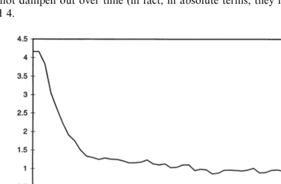
. The run presented here has the following parametrization: k=12, 6=1,d=0.3, l=0.6, a=2,b=6,c=0.02,h=0.04,o=0.5. The demand function is H(x)=4.1667 exp(−0.1x). The random variable z is uniformly dis-tributed over [a, b], j is uniformly distributed over [0, 0.01], and the capitals of newcoming firms are uniformly distributed over [c, h].
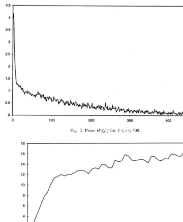
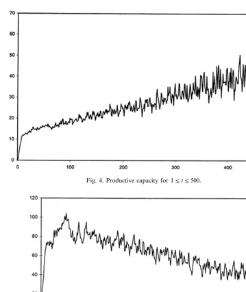
[image:13.612.119.408.300.489.2]Figs. 1 and 2 present the dynamic of prices. While prices decline to 0 with persistent fluctuations, the total productive capacity grows over time with qualita-tively similar fluctuating patterns, whereby the amplitude of fluctuations themselves does not dampen out over time (in fact, in absolute terms, they increase): see Figs. 3 and 4.
Fig. 1. PriceH(Qt) for 15t550.
6A lot of simulations of this kind has been undertaken based on a program from the laboratory for
Fig. 2. PriceH(Qt) for 15t5500.
Fig. 3. Productive capacity 15t550.
for everyone’. At some point, as total supply increases, competitive conditions become more stringent and market selection rather quickly starts affecting growth and survival of lower-efficiency firms7
[image:15.612.84.443.120.546.2]. This change in ‘market selection regime’ is illustrated also by the dynamics of the concentration measures of the industry (see
Fig. 4. Productive capacity for 15t5500.
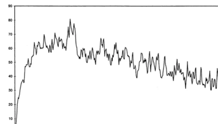
Fig. 5. Total number of firms 05t5500.
7In many respects, the phenomenon recalls the ‘density dependent selection’ emphasized in
Fig. 6. Equivalent number of firms from the Hirfindhal index 15t5500.
Fig. 7. Size distribution fort=50.
Fig. 6 for the ‘equivalent number’ associated with the Hirfindhal index of concentration8
: concentration falls (i.e. the equivalent number increases) up to the ‘shake out’ phase and then increases thereafter. Figs. 7 and 8 provide two
8Callings
i(t) the market share of thei-th firm att, the concentration index is
H(t)=%
nt
i=1
si(t)2.
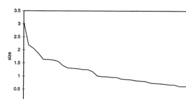
snapshots, measured in terms of productive capacity fort=50 and t=500, where firms are ranked according to their size. What is observed here is something rather close to the Pareto law (see, for example, Ijiri and Simon, 1974)9
[image:17.612.115.417.126.286.2]. Fig. 9 provides the life time distribution of firms for 15t5500 which died before t=500. Life time here means the number of production cycles the firm performs before it dies.
[image:17.612.89.444.240.532.2]Fig. 8. Size distribution fort=500.
Fig. 9. Life time distribution of firms for 15t5500.
9Namely, in one of its versions, for a sample of firms ranked according to their size, the sizesand
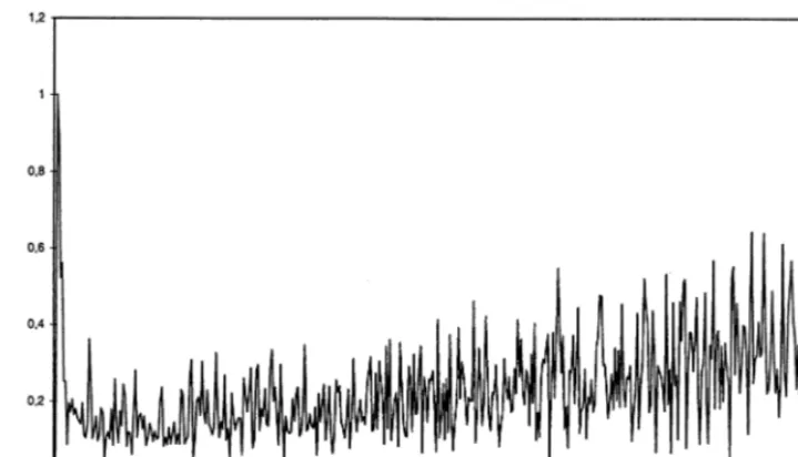
Fig. 10. Turbulence index for 15t5499.
(So for example, in Fig. 9, around 18% of all firms which were born and died before t=500 did die when they were 6-periods old, etc.) Again, the mortality patterns appear to be quite in tune with the evidence, with high mortality rates shortly after birth and a (relative thin) tail of firms with much higher longevity (more on this type of evidence in Hannan and Freeman, 1989; Baldwin, 1995; Geroski, 1995; Carroll, 1997). As known, this survival patterns are sometimes interpreted — especially in the ‘organizational ecology’ perspective — as the outcome of the differential adaptation of subsets of firms in the population. Notwithstanding the likely importance of the latter phenomena, our results here seem to suggest that a distribution of mortality rates which peaks in the early infancy, with a long but thin tale of old survivors might be a rather generic property of a large class of evolutionary processes characterized by heterogenous entry and market selection (cf. also the simulation results in Winter et al., 1997)10.
Finally, Fig. 10 vividly illustrates the evolutionary proposition that whatever persistent regularity emerges in the aggregate, that is likely to be the collective outcome of an ever-lasting microeconomic turbulence. Define a ‘turbulence index’
T(t)= %
nt
i=1
si(t)−si(t+1)+% k j=1
exp{At}u tk+j
/ztk+j.
that is, the sum of the absolute values in the changes of market shares from one period to the next (including gross entry att). As Fig. 10 shows, market turbulence persists — and, if anything tends to increase, throughout the history of the industry.
10A fortiori, one should expect this property to apply also to those circumstances wherein also
3. An alternative dynamic setting: increasing productivity of labor
3.1.Main assumptions
Now we turn to symmetric opposite assumptions compared to the model above and assume that learning concerns only labor productivity11. As above, we have an
industry evolving in discrete timet=0, 1, …. Att=0 there are no firms ready to manufacture, butkfirms come to the industry. They will start producing at t=1. At timet]1 the industry consists ofntfirms which are involved in manufacturing
and new firms that enter at t and will participate in the production process from t+1 on. As in the earlier version of the model we have uniformly for the whole industry:
6 — price per unit of physical capital, 6\0, d — depreciation rate, 0Bd51,
C — capital per unit of output,C\0.
Here, however, the competitiveness of any firm in the industry is determined by its variable costs per unit of output. Let us designate it bymifor the i-th firm. In
this competiti6e en6ironment only newcomers learn how to impro6e(in probability)the
producti6ity of labor. As time goes on the lowest variable costs present in the
industry decreases. In particular, we have the following stochastic mechanism defined endogenously.
Consider a random variablej with positive mean zand a finite varianceDj. Setz for a random variable distributed over [a, b], 0BaBbB . For each time instantt]0 allow for the industry to havek]1 new firms whose variable costs are randomly determined as exp{−At}zitk+15i5(t+1)k. HereAt+1=At+jt+
1
,
t]0,A0=j
0
. Also,jt
,t]0, andzi
,i]1, are mutually independent collections of realizations of j and z. One sees that all variable costs feasible for newcomers at timetbelong to [exp{−At}a, exp{−At}b]. Their distribution over this interval is
governed by a realization of exp{−At}z. Thus At characterizes in a probabilistic
manner the highest productivity of labor attainable by newcomers in the industry at timet.
Alike the model above there is a decreasing continuous demand function p=H(q), mapping [0,) in [0,H(0)] such thatH(0)B andH(q)0 asq .
SetQt
i for the productive capacity of the i-th firm and m
ifor its variable costs.
Then
Qt=%
nt
i=1
Qti, t]1, Q0=0,
is the total productive capacity involved in manufacturing att. The gross profit per unit of output at t for the i-th firm is obviously H(Qt)−mi. Its total gross
investment per unit of capital islmax[H(Qt)−mi, 0]/6C. As above, the constantl
captures the share of the gross profit which is re-invested.
11An assumption, which, together with the constancy of capital/output ratios, seems nearer the
empirical evidence.
For each value of variable costs generated att we shall allow a single entrant. The initial capitals of entrants are independent realizationsui,
i]1, of a random
variableudistributed over [c, h], 0BcBhB . It is assumed that the realizations
of j, z and u are mutually independent random variables.
Again, as above, the death mechanism implies that a firm is dead at timetand does not participate in manufacturing from t+1 onward if its capital at t is less thanoc,o(0, 1]. The situation without mortality corresponds to the limit case when
o=0.
3.2.A dynamic balance equation for industry e6olution
Consider a firmithat is manufacturing at timet. Our investment rule implies that at the end of this production period its capital reads
Qt i
C
!
1−d+ l6Cmax[H(Qt)−mi, 0]
"
.If this value does not drop below the death threshold oc, the firm continues to manufacture att+1. Otherwise it dies12. Hence
Qti+1=Qt
i
!
1−d+l6cmax[H(Qt)−mi, 0]
"
xQti!
1−d+l6Cmax[H(Qt)−mi, 0]
"
]oc/C(3.1)
where xQ
ti{1−d+l/6Cmax[H(Qt)−mi, 0]}]oc/C is the indicator function of the event that
the firm continues to manufacture given the above death rule and the total productive capacity of the industry involved in manufacturing.
This equation describes the evolution of a single firm in business. In analogy with the formalization of the foregoing section, let us proceed to a dynamic representa-tion of the model that reserves room for all feasible development paths of the industry.
For the spaceR introduced in Section 2, define an automorphism D(·) on R such that
D(q)=D1(
q)
i=2D
i(
q)
n
,withD1(·):R
RR1R2 and Di(·):RRi, i]3. Set
D11(q)=q, D1s(q)=0, 25s52k+1, D21k+j+1(q)=qj1exp{−q}xA j 1(q),
D31k+j+1(q)=
!
qk+j1
1−d+ l
6Cmax
H%
p=1 %
k s−1
qk+s p
−qj
1
exp{−q}, 0
nn
"
xAj 1(q),
12In a possibly more realistic setting one could add a sort of bankruptcy rule stating that firms die,
even when their size is greater thanoc, if their gross profits are negative (i.e. [H(Qt)−mi]B0). However,
Dj
1( q)=qj
i
xA j i(q),
Dk+j i
(q)=qk+j i
!
1−d+ l
6Cmax
H %
p=1 %
k s−1
qk+s p
−qj i
, 0
n
"
xAj 1(q),
where 15j5k,i]2, Aj1
(q) designates the relation
qk+j
1
!
1−d+ l
6Cmax
H%
p=1 %
k s=1
qkp+s
−qj1
exp{−q}, 0
n
"
]oc/CandAji(q) stands for the relation
qk1+j
!
1−d+lC
6 max
H%
p=1 %
k s=1
qkp+s
−qij, 0n
"
]oc/C.We restrict ourselves to vectorsq defined by Eq. (2.2) belonging to
R
+=[0,)
i=1
R+i
n
and setH()=0 for the case when the iterated sum is infinite.
The conceptual interpretation of the automorphism is very similar to the one given earlier on. The 2k boxes contain data concerning cohorts, that is groups of firms which were born simultaneously. The only exception is the first box contain-ing two cohorts and additionally (its first coordinate) the value capturcontain-ing the highest productivity of labor attainable in the industry. In each cohort the firstk coordinates are the variable costs and the lastk coordinates represent productive capacities of corresponding firms. The adjustment rule for productive capacities is the same as in Eq. (3.1). (Again, the indicators prevent from carrying over the data related to dead firms.) The relationAji(
q) means that a firm which is placed at the j-th position of the i-th cohort continues to manufacture given the state of the industryq.
Define infinite dimensional random vectors Yt, t
]0, setting
Y1
t
=jt,
Yi+1
t
=ztk+i,
Yk+i+1
t
=utk+i,
i=1, 2, …,k,
Yj t
=0 j]2k+2.
The evolution of the industry is as follows
q(t+1)=D(q(t))+Yt+1
, t]0, q(0)=Y0
, (3.2)
Since Yt
are independent in t, this expression defines a Markov process on R
+.
Moreover, it is homogeneous in time since the deterministic operatorD(·) as well as the distribution ofYt do not depend on time.
3.3.Long run beha6ior of the industry
As above, Doeblin’s condition holds here if we setf(A)=P{Y*AA1} for a
setA given by Eq. (2.4). Here Y* designates a (2k+1)-dimensional vector whose coordinates coincide with first 2k+1 coordinates of a generic vectorYhaving the same distribution as Yt, t]0. The following result establishes the ergodicity of
process Eq. (3.1).
Theorem 3.1. For e6ery setA gi6en by Eq. (2.4) with probability one
1
n %
n t=1
pt(Y0
,A)p(Y0
,A) (3.3)
as n . Herep(Y0, ·) is a stochastic probability measure(since it depends onY0),
beingp£(·)for an elementary outcomevVas long asY0belongs for this elementary
outcome to an ergodic set £.Moreo6er,pt(·, ·)
designates the transition probability in
t steps of process(3.2).
The implications of this theorem in terms of path-dependency (or lack of it) are identical to those discussed above with reference to Theorem 2.1.
Theorem 3.1 implies that for every uniformly bounded characteristic of the industry its time averages converge with probability one to a limit which is a deterministic function of the initial state in the sense given above.
Let us now show that the total productive capacity of the industry is uniformly bounded. Since the minimal size of a firm is bounded by the death threshold, this implies uniform boundedness of the total number of firms in business (if o\0). Hence, we shall be able to derive relations similar to those given in Winter et al. (1997) on convergence of time averages regarding some important characteristics of the industry.
Set Q( =H−1(
d6C/2l) and Q. =max(Q( , 2kh/Cd), where H−1(·) designates the
inverse function.
Lemma 3.1.With certainty Qt5Q*for t]1,where Q=Q. [1+lH(0)/6C]+kh/C.
Proof. Notice thatQ15kh/C5Q*. Eq. (3.1) and the assumption concerning the
entry process imply that
Qt+15Qt
1−d+l
6CH(Qt)
n
+ khC , t]1.
IfQt]Q. for some t]1, we get that Qt+15Q. . Otherwise, if QtBQ. ,
Qt+15Qt
1+l
6CH(Qt)
n
+ khCBQ.
1+l
6CH(0)
n
+ khC .
The lemma is proved.
Corollary 3.1. With probability one
1
n %
n t=1
Qt
&
R0+
%
i=1 %k
p=1
yk+p i dp(
Y0, y)
and, ifo\0,
1
n %
n t=1
6t
&
R0+
%
i=1 %
k p=1
xA
pi(y)dp(Y
0,y)
asn . Here6tdesignates the number of firms in business att. Also, for a vector
q given by Eq. (2.2)
R0 +
=
!
qR+: %
i=1 %
k p=1
qk+p i
5Q
"
.The relationAp i
(y) is defined as above.
Indeed, the infinite sum involved in the first limit is bounded byQ by Lemma 3.1. The sum involved in the second limit does not exceed CQ/ocB if o\0.
Let us turn to the death process.
Theorem 3.2.Ifo\0,then each firm dies in a finite random time with probability one.
The proof is given in the Appendix. The intuition is the following.
For simplicity letoB1. (If o=1, we need a more complicated argument.) Each firm comes with a capital that exceeds c. If it dies, at the moment when this happens its capital does not exceedoc. Since firms with lower variable costs per unit of output have higher investment rates, a notional firm that lives infinitely long would shrink at leasto times during the lifetime of a generic firm characterized by the lowest variable costs per unit of output at some particular time (which nonetheless dies in a finite time). Consequently, to prove that no firm can live infinitely long, it is enough to show that: (a) the capital of every alive firm is bounded from above by a constant; and (b) for every level of variable costs per unit of output there is an infinite chain of firms with lower variable costs that are coming and dying one after another.
The capital of an alive firm is bounded from above by the total capital of the industry which, in turn, is bounded with certainty. Thus, (a) holds. The capital of an alive firm is bounded from below by the death threshold and the total capital of the industry is bounded with certainty. Hence the total number of alive firms is bounded with certainty. Consequently, starting from a finite random timet every newcoming firm dies in a finite time. According to the postulated learning rule, for every given level of variable costs per unit of output, all newcoming firms have lower variable costs starting from a finite random time t%. Thus, from max(t, t%) onward we have the chain required by (b).
H−6Cd/lwill unboundedly grow. Hence, starting from a finite random time with probability one every newcomer will never die, but rather unboundedly grow. The intuition behind this property is the following. AsH(x) approaches its asymptotic value, demand elasticities grow and so does the ‘carrying capacity’ of the market. Correspondingly, selective pressures get weaker. Since output prices have a positive lower bound, if gross margin are high enough (that is if variable costs are low enough) as to sustain positive net investments, then firms which fulfil these conditions will indefinitely survive (and indeed grow), irrespectively of the fact that an infinite number of even more efficient firms will enter thereafter. One will still observe a dynamic on market shares (with all firms having eventually their shares tending to zero), but given an infinitely expanding market, the number of firms will also be allowed to infinitely grow, and mortality will cease to operate as a selection device. Moreover, the total productive capacity of the economy will also grow in the foregoing circumstances faster thangt
ast for every 0BgB1−d+lH/6C but slower than (1−d+lH/6C)t. In these circumstances, (1
−d+lH/6C)t
estab-lishes the upper bound of all feasible rates of growth, with history selecting among them. Hence, some (bounded) path-dependency property of industrial dynamics reappears, as soon as the size of the market is allowed to endlessly grow.
3.4.A numerical run of the model
Let us turn again to an illustration with a computer simulation (for details cf. footnote 6, above).
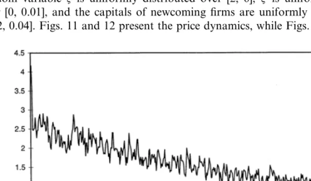
[image:24.612.114.417.398.574.2]The run presented here has the following parametrization:k=12, 6=1,C=2, d=0.3, l=0.6, o=0.5. The demand function is H(x)=4.1667 exp(−0.1x). The random variable z is uniformly distributed over [2, 6]; j is uniformly distributed over [0, 0.01], and the capitals of newcoming firms are uniformly distributed over [0.02, 0.04]. Figs. 11 and 12 present the price dynamics, while Figs. 13 and 14 show
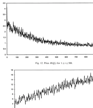
Fig. 12. PriceH(Qt) for 15t5500.
Fig. 13. Total productive capacityQtfor 15t5500.
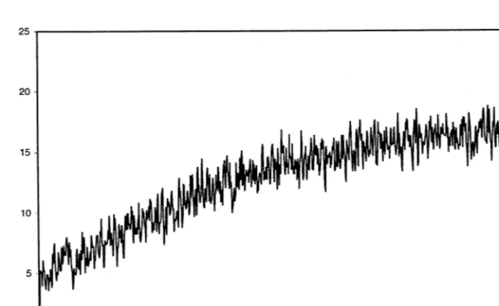
for the same time interval the dynamics of the total productive capacity. The evolution of the total number of firms is shown in Figs. 15 and 16, with Figs. 17 and 18 depicting size distributions at t=50 and t=500. (For prices, productive capacity and number of firms we report also longer simulation runs, witht=1000, for a clearer illustration of the long term properties toward which the system tends to converge.) Fig. 19 provides the life time distribution for firms that die before
Many qualitative properties of the dynamics are similar to those obtained earlier. For example, persistent fluctuations of prices and production capacities and persis-tent market share turbulence (Fig. 20) are a robust feature of both set-ups. And so are Pareto-type size distributions and skewed age profiles. Interestingly, however, no ‘shake-out’ seems to occur in the number of firms at some point in its infancy. In this set-up, notwithstanding the property — given appropriate demand
[image:26.612.84.444.149.370.2]condi-Fig. 14. Total productive capacityQtfor 15t51000.
[image:26.612.93.436.174.564.2]Fig. 16. Total number of firms 05t51000.
Fig. 17. Size distributions att=50.
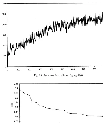
tions — that both productive capacity of the industry and the number of firms have upper bounds, the industry seems to approach them without any major structural discontinuities13 with concentration falling in the long term (Fig.
21).
13A similar profile in the evolution of the number of firms is also obtained, under somewhat similar
Fig. 18. Size distributions att=500.
Fig. 19. Life time distribution for 15t5500. 4. Modeling learning on both capital and labour efficiencies
The two foregoing models may also be combined to account for those (empiri-cally more plausible) circumstances whereby entrants are allowed to innovate, in probability, will respect to both capital and labour efficiencies. In order to define this set-up one needs four random variables:jC, jL, zC, distributed over [aC, bC],
andzL, distributed over [aL,bL]. HereEji\0,DjiB , and 0BaiBbiB ,i=C,
Fig. 20. Turbulence index for 15t5499.
Fig. 21. Equivalent number of firms from the Hirfindhal index for 15t5500.
Set, fort]0
At+1 (C) =A
t
(C)+j
C t+1, A
0
(C)=0, and A
t+1 (L) =A
t
(L)+j
L t+1, A
0 (L)=0.
Allowing for k]1 newcomers at each time, t]0 define their capital ratios and
variable costs as exp{−At
(c)}z c
i and exp{ −At
(L)}z
L i, tk
[image:29.612.87.444.55.461.2]t]0, i=C, L, andzi j,
j]1,i=C,L, are independent (in all indexes) realizations of the corresponding random variables.
For a firmi(whose capital ratio isaiand variable costs aremi) manufacturing at
timet we have as above
Qti+1=Qt
i
!
1−d+ l6aimax[H(Qt)−mi, 0]
"
XQti!
1−d+l
6aimax[H(Qt)−mi, 0]
"
]tc/aiInterestingly, in this set-up productive capacities of newcomers grow to infinity in the same way as in the model with increasing productivity alone. So unboundedly grows the total productive capacity of the industry. Hence, the limit behavior of this industry turns out to be similar to the growth pattern of an industry where newcomers learn how to improve the productivity of capital alone, as in the first of the foregoing models.
5. Conclusions
In this work we have explored some dynamic properties of industrial dynamics driven by an ever-lasting flow of entrants which might, in probability, be carriers of technological innovations (that is, in our simple model, more efficient techniques of production).
Some properties of the ensuing industrial dynamics appear to begenericfeatures of a wide class of evolutionary processes nested into microeconomic heterogeneity and market selection. In particular, (a) persistent fluctuations of aggregate variables — such as price, production capacity, total output — ; (b) turbulence in market shares; and (c) skewed size distributions of firms appear to be robust features of the competitive process, irrespectively of any more detailed characterization of the origins and the bounds upon microeconomic heterogeneity. (In this respect com-pare the results presented here with Winter et al., 1997.) Other properties — corresponding to other empirically observable regularities — depend, on the contrary, upon more specific characterizations of the ways micro heterogeneity is generated. That includes whether and how innovations are generated along the history of the industry.
First, and most intuitively, necessary (but not sufficient) condition for the industry to exponentially grow is the persistent enlargement of notional opportuni-ties of innovation. In the foregoing model the process is represented as an endogenous drift in the set of input coefficients stochastically attainable at each time, conditional on the best-practise knowledge already achieved at such a time. It is an ‘open-ended’ dynamic insofar as, in the limit, there is no bound upon the possibilities of discovery, even if at each time what is attainable is ultimately constrained by what has been learned up to that time.
allow any exogenous demand drift — is that notionally unbounded dynamic increasing returns may fully exert their impact upon output growth only insofar as they are not limited by the extent of the market, to paraphrase the oldadagio by Adam Smith. In the set-up with learning about capital efficiency, the market indefinitely grows in real terms because technical progress provides, for its nature, also a corresponding possibility of expansionary investment in productive capacity. Given the hypotheses of that specification of the model, even if the demand curve does not shift (in nominal terms) over time, capital costs of production per unit of output progressively wither away as time goes on, and, as a consequence, the benefits of increasing returns to knowledge accumulation can be fully reaped throughout.
Conversely, this might not be the case with learning occuring only with respect to labour efficiencies. Here, the long-term evolutionary outcomes depend upon the interplay between the shape of the demand curve and the level of fixed capital costs per unit of output. The latter obviously set a ceiling to the maximum expansion of production capacity from anyttot+1 for whatever gross margin each firm is able to obtain. Whether such a ceiling to micro growth in any finite time carries over to the long-run system properties is, however, a quite different matter. As discussed above, under these circumstances, self-sustained growth of the industry can be attained only if the shape of the demand curve is such as to allow in the long-run an indefinite expansion of total gross surplus and of net investments in production capacity14.
More generally, as both our analytical results and simulations show, the long-run dynamics of the industry depends also on the interplay between patterns of technological learning and demand conditions (this is a point emphasized also in more static set-ups by Sutton, 1998, which turns out to apply in our model even when disposing of any assumption of ‘rational’ consistency amongst microbehaviors).
In this paper we focused upon a specific archetype of learning dynamics, which — in tune with earlier literature — we calledSchampeter Mark I. In such a stylized learning regime, one restricted a positive probability of learning to entrants, with inputs coefficients fixed thereafter for all incumbents. While an obvious violence to a much more messy empirical evidence, this modeling framework allows an easier identification of the properties of that subset of learning processes whereby incum-bent knowledge is highly inertial and the dominant source of change is the arrival of new entrepreneurial trials.
Given the formal Schumpeter Mark I set-up, we show as our third major conclusion that generally the process of competition and collective growth must be fueled by an unending process of entry and exit, with each individual firm dying with probability one in finite time and, whereby, paraphrasing Geroski, the life of each firm tends to be ‘nasty, brutish and short’ — cf. Geroski and Schwalbach (1991) and Geroski (1995). (The only exception we find is under some rather special
14Clearly, the condition would be more easily met if one allowed some positive drift over time in
demand patterns whereby an infinitely growing number of firms can survive, with non-decreasing absolute size, notwithstanding vanishingly small market shares, given exponentially growing markets).
Fourth, with the open-ended innovative dynamics considered here, the role of history, i.e. more formally, path-dependence — more forcefully appears in the account of long-term dynamics. As already noted in Winter et al. (1997). even in a ‘closed’ world of technological options, the expressions for long-term average statistics for the industry contains a possible dependence upon initial conditions (insofar as more than one ergodic set exists, determining the Markovian structure of industry evolution(s)). Here, however, path-dependency acquires much more straightforward implications. In essence, under all conditions whereby the industry unboundedly grows, what one is able to prove,in a history-independent fashion, is that a whole class of exponential functions may fit any pattern generated under these conditions. However, as we show above, path-dependence essentially affects
which growth rateturns out to be selected also in the long-term.
Acknowledgements
We are grateful to Andrea Bassanini, the participants to the Conference on Economic Models of Evolutionary Dynamics with Interacting Agents (The Abdus Salam International Centre for Theoretical Physics, Trieste, Italy, September 1998) and two anonymous referees for their comments on previous drafts. Mariele Berte` and Marco Valente have been of crucial help for the simulation of the model. Francesca Chiaromonte preciously contributed to the endless discussions concern-ing both the fine details of the model and its computer simulations.
We thank the International Institute for Applied Systems Analysis, the Fujitsu Research Institute for Advanced Information (Japan), the University of Trento and the European Union (ESSY Project, TSER, DG XII) which at various stages supported the research leading to this work. Usual caveats apply.
Append