Children’s Achievement
Impacts of State Policies, Family Background,
and Peers
Todd E. Elder
Darren H. Lubotsky
a b s t r a c t
We present evidence that the positive relationship between kindergarten entrance age and school achievement primarily reflects skill accumulation prior to kindergarten, rather than a heightened ability to learn in school among older children. The association between achievement test scores and entrance age appears during the first months of kindergarten, declines sharply in subsequent years, and is especially pronounced among children from upper-income families, a group likely to have accumulated the most skills prior to school entry. Finally, having older classmates boosts a child’s test scores but increases the probability of grade repetition and diagnoses of learning disabilities such as ADHD.
I. Introduction
At what age should children begin kindergarten? During the past 30 years, a steadily increasing fraction of children has entered kindergarten after their sixth birthday instead of the more traditional route of beginning at age five. In
Todd E. Elder is an assistant professor of economics at Michigan State University. Darren H. Lubotsky is an associate professor of economics and labor and industrial relations at the University of Illinois at Urbana-Champaign. The authors thank many seminar participants as well as John Bound, Jeffrey Brown, Ken Chay, Janet Currie, John DiNardo, David Lee, Justin McCrary, Patrick McEwan, Miguel Urquiola, Richard Rothstein, and an anonymous referee for helpful comments. Dan Hanner provided excellent research assistance. The authors gratefully acknowledge financial assistance from the University of Illinois Campus Research Board and the National Institute of Child Health and Human Development under grant R03HD054683. The content is solely the responsibility of the authors and does not necessarily represent the view of the National Institute of Child Health and Human Development or the National Institutes of Health. The authors are willing to offer guidance to other researchers seeking the restricted-use data used in this paper, available by applying to the National Center for Education Statistics.
[Submitted June 2007; accepted April 2008]
ISSN 022-166X E-ISSN 1548-8004Ó2009 by the Board of Regents of the University of Wisconsin System
October 1980, 9.8 percent of five-year-olds were not yet enrolled in kindergarten; by October 2002, that figure had risen to 20.8 percent.1Much of this increase stems from changes in state-mandated cutoff dates that require children to have reached their fifth birthday before a specific day to be eligible to begin kindergarten each fall. (For example, in Illinois a child must have turned five years old by September 1, 2007 to be eligible to enroll in the fall of 2007.) In addition, many parents of children born in the months before the cutoff choose to hold their children out of kindergarten for a year. These children would have been the youngest in their kindergarten class if they began when first allowed to enroll, but instead are among the oldest children in the class that begins the following academic year. These policy reforms and parental choices are largely based on research showing that children who are older when they start kindergarten tend to do better in early grades, perhaps justifying the large price these children pay through delayed entry into the labor market.2
The evidence in this paper presents a contrarian view: Age-related differences in early school performance are largely driven by the accumulation of skills prior to kindergarten and tend to fade away quickly as children progress through school. Rather than providing a boost to children’s human capital development, delayed en-try simply postpones learning and is likely not worth the long-term costs, especially among children from poorer families and those who have few educational opportu-nities outside of the public school system.
Parents, educators, and researchers have long understood that older children tend to do better across a variety of measures than younger children within the same grade. In the early 1930s, the Summit, New Jersey school system was inter-ested in determining which students to admit into first grade. To help answer this question Elizabeth Bigelow (1934) studied the achievement of 127 fourth graders in the school system, found that children who were older when they began first grade were less likely to repeat one of the first three grades, and also tended to score higher on the Modern School Achievement Test. These achievement differ-ences have been validated recently with arguably better samples and statistical techniques. It is perhaps surprising that there is little research about the mecha-nisms that lead these gaps to emerge, whether delayed entry passes a reasonable cost-benefit test, and what the implications are for education policy and parental decisions.
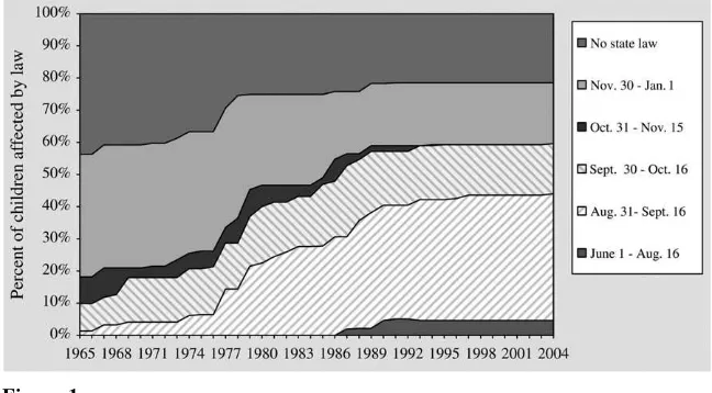
Despite our poor understanding of the consequences of delayed kindergarten enrollment, states have been moving their entry cutoffs earlier in the fall in order to raise the average entrance age. Figure 1 shows the population-weighted fraction of states with entrance cutoffs in six selected categories. In 1975, six states had cutoffs of September 14 or earlier, while 14 states had relatively late cutoffs be-tween November 30 and January 1. An additional 15 states did not have any uni-form state regulation and instead left such decisions up to individual school
1. These figures come from tabulations of the 1980 and 2002 October Supplements to the Current Popu-lation Survey.
districts. From the mid-1970s to the mid-1990s, many states either moved their kindergarten birthday cutoff from December to September or instituted a Septem-ber cutoff when there previously was no statewide mandate. By 2004, 29 states had cutoffs of September 14 or earlier, five states had cutoffs between November 30 and January 1, and only eight states had no uniform state law.
There are two broad reasons why older children do better than their younger classmates, each with different policy implications. The conventional wisdom is that older children are more likely to have the necessary skills and maturity to succeed in school and therefore learn more in each grade. An important impli-cation of this interpretation is that age-related differences in eduimpli-cational out-comes will tend to persist or grow as children progress through school, so that the decision to begin kindergarten at an older age could be a worthwhile investment: Older entrants potentially learn more in school, go further in school, and enter the labor market with more human capital than they otherwise would have.
An alternative view is that age-related differences in early school performance stem solely from prekindergarten learning. Once children begin kindergarten, ac-cording to this view, older and younger children tend to learn at the same rate. The skill differences that existed prior to kindergarten tend to fade away as they come to represent a smaller fraction of children’s overall stock of knowledge and skills. Parents who hold their child out of school, or states that adjust their entrance requirements to raise the average entrance age, will raise achievement in early grades with little or no long-term benefit to compensate for the high cost paid in terms of Figure 1
State Entrance Age Cutoffs, 1965-2005
lost future working years, additional childcare costs, and potentially reduced educa-tional attainment.3
We use two sources of data, the Early Childhood Longitudinal Study-Kindergarten cohort (ECLS-K) and the National Educational Longitudinal Survey of 1988 (NELS:88), to shed light on the mechanisms underlying the relationship between school performance and the age at which children begin kindergarten. Compliance rates with state entrance cutoffs are high in both data sources, implying that the changes in state laws have had powerful effects on the timing of kindergarten en-trance. We exploit the fact that these cutoffs generate individual-specific entrance ages that are arguably exogenous with respect to school performance to measure the relationship between entrance age and outcomes.4 For example, a child born in October who lives in a state with a December 1 cutoff may begin kindergarten in the fall that he turns five years old, while an otherwise similar child that lives in a state with a September 1 cutoff would have to wait an additional year to enter kindergarten. Variation in birthdates throughout the calendar year among children who live in the same state and face the same entrance cutoff generates additional var-iation in age at kindergarten entry. Based on these two distinct sources of varvar-iation in entrance age, we use children’s predicted kindergarten entrance age if they were to begin school when first allowed by law as an instrumental variable for children’s actual kindergarten entrance age in models of reading and math test scores, grade progression, and diagnoses of a variety of learning disabilities including Attention Deficit / Hyperactivity Disorder (ADD/ADHD).5
Three empirical findings point to prekindergarten preparation, rather than learning during kindergarten, as the mechanism underlying the entrance age effect. First, our baseline models indicate that being a year older at the beginning of kindergarten leads to a 0.53 standard deviation increase in reading test scores and a 0.83 standard deviation increase in math scores during the fall of kindergarten, a point in time so early in the academic year that very little learning could have taken place in school. Second, we present compelling evidence that entrance age effects are much larger and more persistent among children from high socioeconomic status families. This
3. Angrist and Krueger (1992) point out that younger entrants reach the compulsory schooling age having completed more schooling than older entrants. Their empirical analyses of the 1960 and 1980 Censuses indicate younger entrants complete more schooling than older entrants. Dobkin and Ferreira (2006) reach a similar conclusion with more recent data. By contrast, Bedard and Dhuey (2006) and Fredriksson and O¨ ckert (2005) show the opposite, while Fertig and Kluve (2005) find no relationship between entrance age and schooling.
4. Most state cutoffs have provisions that allow children to begin a year earlier than proscribed by law if granted permission by local school administrators. Permission is generally not needed to delay kindergarten entry. State entrance laws apply only to public schools; children who attend private schools are not bound by the state cutoffs.
pattern is consistent with a relatively fast rate of accumulation of human capital among high-income children in the years prior to kindergarten.
Finally, as children progress through school, achievement gaps between older and younger children tend to fade away, consistent with the gaps being relics of prekin-dergarten learning. If older children were able to learn at a faster rate, one would ex-pect the achievement gaps to widen from one year to the next. By third grade, there is no statistically significant association between entrance age and test scores among the poorest children. Although the entrance age effects among the most advantaged children persist until at least eighth grade, they are only a fraction of the gradient seen in kindergarten.
Even though test score gradients fade away over time, teachers, parents, and school administrators appear to make important decisions based on these early differ-ences: Being a year younger at entry raises the probability of repeating kindergarten, first, or second grade by 13.1 percentage points, a sizeable effect relative to the 8.8 percent baseline retention rate. Similarly, being a year younger at entry raises the probability of being diagnosed with Attention Deficit/Hyperactivity disorder by 2.9 percentage points, which is also large relative to the 4.3 percent baseline diagno-sis rate.
We present evidence that the age of a child’s peers also has important effects on test scores, grade progression, and diagnoses of learning disabilities. Differences in entrance cutoffs across states generate potentially exogenous variation in the average age of kindergarten students within a school. We use this variation to show that, con-ditional on a child’s own age, having older classmates tends to raise reading and math achievement but also increases the probabilities of repeating a grade and re-ceiving a diagnosis of a learning disability such as ADD/ADHD. For example, we estimate that moving a kindergarten cutoff from December 1 to September 1 in-creases ADD/ADHD diagnoses by approximately 25 percent of the baseline rate among children whose own entrance age is unaffected because these children are now younger relative to their classmates. These negative peer effects likely arise from the fact that grade progression and the decision to refer a child to a behavioral specialist are partly based on judgments about how a child compares to his or her classmates, rather than based solely on an absolute standard.
Our estimates clearly indicate that children’s reading and math abilities increase much more quickly once they begin kindergarten than they would have increased during the same time period if they delayed kindergarten entry. In the absence of a future policy that dramatically increases the accumulation of skills prior to kinder-garten entry, increases in kinderkinder-garten entrance ages have the primary effect of delaying the rapid learning that children experience once they begin school, espe-cially among those from low-income households.
II. The Origin of the Kindergarten Entrance Age Effect
human capital, ht-1, and new human capital acquired through parental investments and through schooling:
ht¼bht21+ItðYÞ+utðS;EAÞ:
ð1Þ
ItðYÞ are the per-year investment of parents in the human capital of their children, which is a function of parental resources,Y. Parental investments include any learn-ing that takes place prior to kindergarten, includlearn-ing the choice to enroll a child in a preschool program. Following past empirical and theoretical literature, we assume that parental resources are positively associated with parental investment, so @ItðYÞ=@Y.0.utðS;EAÞis the contribution of yearSof schooling to human capital for a child who entered kindergarten at age EA. The return to schooling (at least for early grades) may be larger for children who are older at entry, so that @utðS;EAÞ=@EA$0, which captures the idea of ‘‘kindergarten readiness.’’6 ut also could depend on classmates’ ages if, for example, lessons are geared to the average child. We study the effect of class average age,EA, on achievement in Section VII. Without loss of generality, we assume initial investments and human capital are zero,
h0¼I0¼0. (To economize on notation, we have suppressed an individual sub-script.) In this framework, skills depreciate at the rate of (1-b).
This model delivers three important predictions about the relationship be-tween kindergarten entrance age, socioeconomic status, and school achieve-ment: first, gaps in achievement between older and younger kindergarteners will be evident at the beginning of the school year. On the first day of kindergar-ten, children’s human capital consists only of previous parental investments and is given by:
hEA¼+ EA
j¼0
bjIEA2jðYÞ
ð2Þ
Children who are older at the beginning of kindergarten will tend to be more skilled because they will have had more time to accumulate human capital during their pre-school years. The youngest child in a typical kindergarten classroom tends to be about five years old, a full year younger than the oldest child in the classroom. This one year age difference represents a potentially large difference in prekindergarten learning. Formally,@ht=@EAjt¼EA¼IEA21ðYÞ, which captures the influence of addi-tional parental investments prior to schooling on human capital at the beginning of kindergarten. One interpretation of this relationship is the entrance age effect among new kindergarten entrants captures the causal effect of a year of parental invest-ments.
The model also predicts that the positive relationship between entrance age and achievement will be larger among children from high socioeconomic families, as long as parental investments are positively associated with parental resources (@2ht=@EA@Yj
t¼EA.0). Because children in higher socioeconomic families learn
at a faster rate, the additional year of learning prior to kindergarten produces a larger difference in skills between older and younger children in rich families than in poorer families. Put differently, exogenous variation in entrance age potentially allows us to measure the differences between rich and poor families in the causal effect of an ex-tra year of parental time and resources prior to kindergarten.
Once children begin school, differences in achievement between children with dif-ferent entrance ages may result from differences in the return to schooling, differen-ces in contemporaneous parental investments, and differendifferen-ces in prekindergarten skills. For example, human capital one year after kindergarten entry is given by:
hEA+1¼bhEA+IEA+ 1ðYÞ+uEA+ 1ð1;EAÞ:
ð3Þ
The first term,bhEA, represents skills acquired prior to the start of kindergarten, the second term represents parental investments made during the first year of school, and the third term,uEA+1ð1;EAÞ, represents the contribution of the first year of schooling to children’s human capital. Because all three of these terms are potentially corre-lated with a child’s entrance age, estimates of differences in achievement bet-ween older and younger children in later grades by scholars from Bigelow (1934) to Bedard and Dhuey (2006) confound the ability to learn while in school
ð@utð1;EAÞ=@EAjt¼EA+1Þwith the differences in ability that existed prior to kinder-garten.7
Finally, the model has important implications for the long-run impact of entrance age on skills and achievement. Human capital afterkyears of school attendance is given by
The effect of a one-year increase in kindergarten entrance age on human capitalk
years after school entry is then
@ht
Ignoring parental investments after children begin schooling, kindergarten entrance age may have a lasting effect on human capital for two reasons: First, the effects of skills acquired prior to kindergarten entry by older entrants may fade away at a slow rate (ifb ¼0.9, 43 percent of differences in prekindergarten learning will still be noticeable after eight years of schooling). Entrance age effects also may persist if older entrants learn at a faster rate during some grades, so that
@utðj;EAÞ=@EAjt¼EA+j.0. Our final test of whether the relationship between en-trance age and achievement is primarily driven by prekindergarten learning or by heightened ability to learn in school is to test whether differences in performance be-tween older and younger entrants expand from one year to the next, at least during the initial years of school.
III. Data
We analyze two sources of data: the Early Childhood Longitudinal Study-Kindergarten cohort, a nationally representative survey of kindergarteners in the fall of 1998, and the National Educational Longitudinal Study of 1988, a nation-ally representative survey of eighth graders in the spring of 1988. This section describes the data and sample construction. Sample statistics are given in Appendix Table A1.
A. The Early Childhood Longitudinal Study (ECLS-K)
ECLS-K is a National Center for Education Statistics (NCES) longitudinal survey that began in the fall of 1998. The NCES initially surveyed 18,644 kindergarteners from over 1000 kindergarten programs in the fall of the 1998–99 school year. Indi-viduals were resampled in the spring of 1999, the fall and spring of the 1999–2000 school year (when most of the students were in first grade), and again in the spring of 2002 and 2004 (when most were in third grade and fifth grade, respectively). Child-ren’s parents, teachers, and school administrators were also interviewed. We use a base sample of 14,333 children who have data from at least two different interviews and nonmissing information on state of residence.
Kindergarten entrance age is computed as the child’s age on September 1 of the year he or she began kindergarten. Although the ECLS-K contains information on kindergarten cutoff dates at the school level, as reported by a school administrator, we opt to use kindergarten cutoffs that are set as part of state law.8 School level cutoffs, especially for private schools and for all schools in states without a uni-form statewide cutoff, are potentially correlated with the socioeconomic status of parents or the ability level of children. Statewide cutoffs are less likely to suffer this source of bias (we return to the issue of the exogeneity of state cutoffs below and in the Appendix). We assign to each child the kindergarten cutoff in his or her state of residence in the fall of 1998, listed in Appendix Table A2. Some states do not have uniform state cutoffs (commonly known as ‘‘local education authority option’’ states), so we exclude children living in those states from our analysis. We compute predicted entrance age, our key instrument, as the child’s age on Sep-tember 1 in the year he or she was first eligible to enter kindergarten according to the state cutoff. Although private schools are not bound by the state kindergarten policies, we include children who attend private schools in our sample (and
compute their predicted entrance age using the public school cutoff) since the de-cision to attend a private school is plausibly related to the local public school’s entrance policies.
Our central outcomes are children’s performance on math and reading tests ad-ministered in each wave and indicators that a child is retained in grade or diag-nosed with a variety of learning disabilities. We use item response theory (IRT) and percentile test scores to facilitate comparability of scores across individuals and over time. The IRT method of test scoring accounts for the fact that the dif-ficulty level of exam questions depends on how well a student answered earlier questions on the test and on the student’s past test performance. We compute each child’s percentile rank among all children who took the same test in the same year (for example, the percentile among all reading tests taken in the spring of 2000, regardless of the child’s grade). Our measure of grade retention is an indicator that the child was in either first or second grade during the spring 2002 interview, when he or she would have otherwise been in third grade. Finally, parents are asked in each survey whether their child has been diagnosed with any of a series of learning disabilities, including attention deficit disorder (ADD), attention deficit-hyperac-tivity disorder (ADHD), autism, and dyslexia. We create three separate indicators: one for whether a child was diagnosed with any learning disability, one for whether a child was diagnosed with ADD or ADHD, and one for whether a child was diagnosed a disability other than ADD or ADHD. ECLS-K provides a host of questionnaire and longitudinal weights for each follow-up, but because our results are largely insensitive to the use of sample weights, we present unweighted esti-mates throughout.
B. The National Educational Longitudinal Study of 1988 (NELS:88)
NELS:88 is an NCES survey, which began in the spring of 1988; 1,032 schools con-tributed as many as 26 eighth-grade students to the base year survey, resulting in 24,599 eighth graders participating. Parent, student, and teacher surveys provide in-formation on family and individual background and on pre-high school achievement and behavior. Each student was also administered a series of cognitive tests to ascer-tain aptitude and achievement in math, science, reading, and history. We again use standardized item response theory (IRT) and percentile test scores. Our central out-come measures are the eighth grade reading and math test scores and an indicator of whether an individual repeated any grade up to eighth grade. As in the ECLS-K, our results from NELS:88 are not sensitive to the use of sample weights, so we present unweighted estimates below.
Unlike the ECLS-K data, in the NELS:88 we do not know where a student lived when he or she entered kindergarten, nor the year they actually began kindergarten. We assign them the state cutoff in effect at the time of their kindergarten entry in their 1988 state of residence and calculate predicted entrance age in a similar manner to that in the ECLS.9This assignment induces some measurement error in predicted
entrance age, but not actual entrance age, resulting in a decrease in the precision of IV results.10The consistency of the estimates is not affected. We assume children began kindergarten in the fall of 1979 if they had not skipped or repeated grades prior to the eighth grade interview. The NELS includes retrospective reports on grade pro-gression, which we use to calculate the year of kindergarten entry for kids who skip-ped or repeated a grade.11Kindergarten entrance age is computed as the child’s age on September 1 in the year he or she entered kindergarten. Again, we exclude from our analyses children living in states without a uniform kindergarten cutoff.
IV. Using Predicted Entrance Age to Identify the
Entrance Age Effect
In this section, we discuss methods to identify the relationship be-tween entrance age and children’s outcomes. We begin with an intuitive description of our research design, then present the formal instrumental variables framework. The final subsection presents baseline estimates of the relationship between test scores and entrance age.
Variation in kindergarten entrance age potentially stems from three sources: First, the distribution of birthdates throughout the calendar year leads to variation in entrance age among children who begin kindergarten when first allowed by their state’s entrance cutoff. Second, differences across states in kindergarten en-trance cutoffs create variation in kindergarten enen-trance ages among children with the same birthday who live in different states. Finally, some children begin kinder-garten earlier or later than proscribed by their state entrance cutoff. This can hap-pen either because a child goes to a private school or because a parent petitions the local school for an exception to the state cutoff. Our research design estimates the relationship between entrance age and outcomes based only on the first two sources of variation, because these sources produce variation in entrance age that is arguably unrelated to other factors that influence children’s outcomes (this iden-tification assumption is discussed in more detail below). By contrast, parental decisions to delay or expedite their child’s kindergarten entry are almost certainly related to other characteristics of parents and children. For example, children who begin kindergarten early are likely to be particularly skilled or gifted, while parents of children with developmental problems are likely to delay their child-ren’s enrollment.
A. The Reduced-Form Relationship between Entrance Age and Outcomes
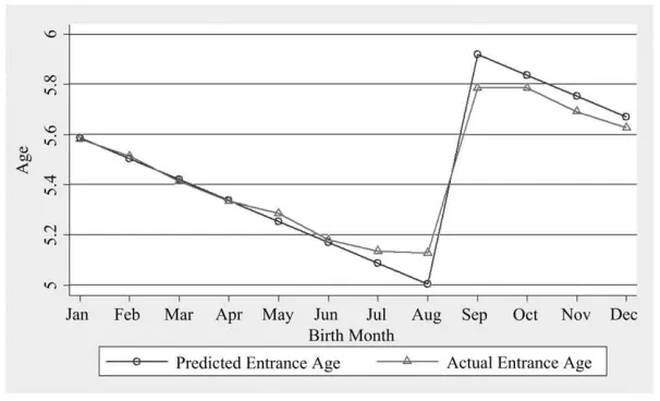
Figure 2 shows the relationship in the ECLS-K between birth month, average actual entrance age, and average predicted entrance age in states with a September 1 cutoff. Recall that we define predicted entrance age as the children’s entrance age if he or
10. Lincove and Painter (2006) also discuss this source of measurement error.
she started kindergarten in the year first allow by law.12Among children born before September 1, variation in birth month is associated with a month-for-month decrease in predicted entrance age. Children born in September, however, are born after the cutoff and are required to wait until the following fall to enroll in kindergarten. Hence, predicted entrance age jumps by 11 months between those with August birth-days and those with September birthbirth-days. Noncompliance on either side of the en-trance cutoff reduces the size of the discontinuity in average enen-trance age to less than 11 months, but the laws clearly exert a powerful influence on actual entrance decisions.
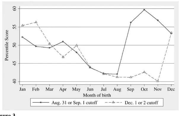
The discontinuity in entrance age is mirrored by a discontinuity in academic performance. Figure 3 shows the relationship in the ECLS-K between birth month and fall kindergarten math percentile scores in states with August 31 or September 1 cutoffs and states with December 1 or 2 cutoffs. In states with December 1 or 2 cutoffs, the oldest children in the class are born in December and the youngest children are born in November. Math test scores are steadily declining from one birth month to the next in these states, but with a sharp increase in scores between November and December births. Those with November birthdays score about 13.2 percentile points lower than their classmates with December birthdays, implying a one-year entrance age effect of 14.4 percentile points (¼ 13.2 / (11/12)). By Figure 2
Average Predicted and Actual Entrance Ages by Birth Month in States with Septem-ber 1 Cutoffs, ECLS-K
contrast, in states with an August 31 or September 1 cutoff, children born in Au-gust are the youngest in the class, while those born in September are the oldest. In these states, there is a clear discontinuity in test scores between kids born in Au-gust and those born in September, with the 14.1 percentile point differential cor-responding to a one-year entrance age effect of 15.4 percentile points. In unreported tabulations, we find a similar pattern with reading scores.
We also note that across-state variation in the entrance cutoff generates differences in the average entrance age within schools or classes. The average entrance age in states with an August 31 or September 1 cutoff is 5.45 years, while the average en-trance age in states with a December 1 or 2 cutoff is 5.25 years. In Section VII, we focus on across-state differences in entrance cutoffs to identify separately the influ-ence of a child’s own entrance age on his or her outcomes from the influinflu-ence of peers’ average entrance age on outcomes.
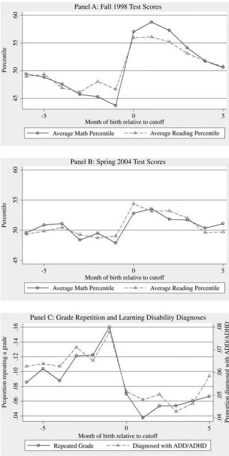
Figures 4a and 4b combine within- and across-state variation in entrance age and show the reduced-form relationships between a child’s birth month relative to statewide cutoffs and average reading and math percentile scores. Figure 4a shows data from the fall of 1998, when children first begin kindergarten. The old-est entrants, born after their state’s cutoff but in the same month, have a value of ‘‘month of birth relative to cutoff’’ of zero and score at roughly the 57th percentile on the math test and the 56th percentile on the reading test.13 The youngest entrants, born before their state’s cutoff in either the same month or the previous Figure 3
Fall Kindergarten Math Scores by Month of Birth, ECLS-K
Figure 4
month, score at approximately the 44th percentile on math and 47th percentile on reading, on average. Apart from the sharp discontinuities among children born near the cutoff, we cannot reject that the relationship between test scores and birth month relative to cutoff is linear. The discontinuity in test scores around the en-trance cutoff is noticeably smaller in the spring of 2004 (Figure 4b), when ontrack children are in fifth grade. The youngest entrants score at the 48th and 49th per-centiles in math and reading, respectively, while the oldest entrants score at the 53rd and 54th percentiles.
Finally, Figure 4c illustrates the reduced-form relationship in ECLS-K between birth month relative to entrance cutoffs and the probability of being diagnosed with a learning disability or repeating a grade in school by grade three, respectively. As in the pattern for test scores, there is a strong relationship between birth month relative to the cutoff and these outcomes, with a large discontinuity between the oldest and youngest predicted kindergarten entrants. Specifically, the youngest children are di-agnosed with learning disabilities at a nearly 50 percent higher rate than the oldest children (note that the figure includes two vertical axes). Among children born just before the cutoff date, the fraction who repeats a grade in school is over 16 percent, nearly triple the grade repetition rate of those born in the months after the cutoff.
Figures 2 through 4 illustrate the essence of the identification strategy we will pur-sue. If birthdays and kindergarten cutoff dates are exogenous with respect to test scores, grade retention, and learning disability diagnoses, variation in entrance age across predicted entrance ages can identify the causal effect of entrance age on these outcomes. Our main results below use both within-state and across-state sources of variation in entrance ages simultaneously.
B. Baseline Instrumental Variables Model
Our identification strategy uses a child’s kindergarten entrance age if he or she began kindergarten when first allowed by state law as an arguably exogenous source of var-iation in his or her actual entrance age. The baseline model is given by the system
Yi¼aEAi+Xig+ei
ð6Þ
EAi¼bPEAi+Xid+ni
ð7Þ
whereiindexes children,Yiis the outcome of interest,EAiandPEAiare actual and predicted entrance age, and Xi represents a vector of demographic, family back-ground, city type, region, and child characteristics that may influence outcomes and actual entrance age.eirepresents unobserved determinants of outcomes, includ-ing cognitive or noncognitive skills, and ni represents unobserved determinants of children’s entrance age, which also may include a child’s ability and maturity, as well as parental characteristics.14The coefficientarepresents the average effect of en-trance age on outcomes. OLS models of Equation 6 will deliver consistent estimates
14. Because actual entrance age and predicted entrance age will always differ by a whole year (or two in rare cases), one can think ofXid+niin Equation 7 as being a linear approximation to a function that takes
ofaif Covðei;EAijXiÞ ¼0, a condition which is not likely to be satisfied because parents choose whether to start a child in kindergarten on time, delay entry, or enter early based on the child’s maturity and ability.ais identified in instrumental vari-ables (IV) models if Covðei;PEAijXiÞ ¼0.
Our covariates include indicators for gender, race, ethnicity, family structure, the marital status of the child’s primary caregiver, Census region, urbanicity, parental education, household income, family size, and quarter of birth. Since we analyze several years of data from the ECLS-K, our covariates for these models reflect char-acteristics in each year. The covariates in the NELS:88 refer to charchar-acteristics when the child was in eighth grade.
Consistent estimation ofarelies on the exogeneity of both sources of variation in predicted kindergarten entrance ages: differences in months of birth across children and differences in kindergarten cutoff dates across states. Bound and Jaeger (2000) discuss a large body of evidence showing correlations between season of birth and family background, education, and earnings, especially among older generations of Americans. Although we find only small, statistically insignificant associations be-tween family background and children’s quarter of birth, we include quarter of birth indicators in all outcome models. The inclusion of these indicators does not substan-tially affect our parameter estimates, nor does including a linear trend in calendar month of birth or individual month of birth indicators. The identification strategy would also be invalid if parents sort into states based on kindergarten cutoffs, or if states choose their cutoffs based on factors correlated with average characteristics of children in the state. The main results include Census region indicators, which control for regional variation in child ability. Our central findings are robust to the inclusion of state fixed effects, which forces identification to come from within-state variation in birthdates, and to limiting the estimation sample to a ‘‘regression discon-tinuity sample’’ of those born within one month of their state’s entrance cutoff date. Although we do not include the school average entrance age in our baseline models in Section IVC. below, our results in Section VII indicate that the influence of a child’s own entrance age on outcomes is not affected when we also include the school average entrance age in the model. The sensitivity of our results is further ex-plored in the Appendix.15, 16
Finally, note that IV estimation of Equations 6 and 7 does not require full compli-ance with entry cutoffs, nor does it require that noncomplicompli-ance be random. Full
15. Because the sampling frames in our data are a kindergarten entry cohort and an eighth grade cohort, rather than birth cohorts, our models compare children born in different years who entered school at the same time. Following birth cohorts and following kindergarten entry cohorts will not necessarily produce similar estimates if birth year or entry year have independent effects on outcomes. Note also that our results for the NELS are conditional on being in eighth grade, while our ECLS-K results do not condition on child-ren’s grade level.
compliance would imply equality of entrance age and predicted entrance age, so OLS and IV would deliver identical results. Similarly, if noncompliance were random, OLS estimation of Equation 6 would be consistent and there would be no need for IV. In the conclusion, we discuss the implication of our findings for children who do not enter when first allowed by state law. As in all IV models, estimates ofaidentify local average treatment effects (LATE) among children whose actual entrance age is af-fected by their predicted entrance age.17The sensitivity analyses in the Appendix in-dicate that the point estimates are quite insensitive to using very different types of variation in entrance age, identifying different local average treatment effects. This provides some assurance that our findings are applicable to a wide set of children.
C. Baseline Estimates of the Relationship Between Entrance Age and Test Scores
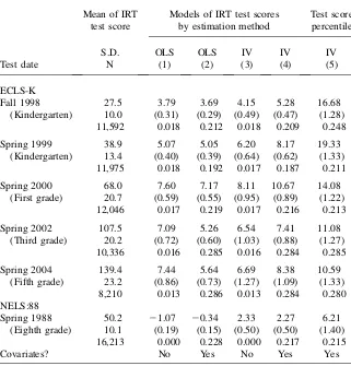
Table 1 presents OLS and IV estimates of the effect of school entrance age on reading test scores from fall 1998, spring 1999, spring 2000, spring 2002, and spring 2004 from the ECLS-K, and from spring 1988 in NELS:88. For a child that follows the normal grade progression, the ECLS-K test dates correspond to the fall and spring of kindergarten, the spring of first grade, the spring of third grade, and the spring of fifth grade. All NELS:88 respondents were in eighth grade in spring 1988. Column 1 shows results from an OLS regression of reading test scores on entrance age with-out any additional covariates. An additional year of age at kindergarten entry is as-sociated with a 3.79-point increase in fall kindergarten test scores, which is 14 percent of the average score of 27.5 and 38 percent of the standard deviation of scores. The associated standard error is 0.31, which is roughly 0.03 of the standard deviation.18Column 2 includes the full set of control variables. The OLS estimate is essentially unchanged, indicating that entrance age is largely uncorrelated with ob-servable determinants of fall 1998 test scores. Columns 3 and 4 present IV estimates with and without control variables. Both of these estimates are larger than the corre-sponding OLS estimates, implying either that delayed entry is more common among students who would otherwise have low test scores or that early entry is more com-mon acom-mong otherwise high-scoring students. The IV estimate with controls shows that being a year older at kindergarten entry increases average fall 1998 test scores by 5.28 points, corresponding to a 0.53 standard deviation effect. Finally, in Column 5 we express the reading test score as a percentile within the ECLS and NELS:88 samples (ranging from one to 100 with a mean of 50), with the IV estimate showing a 16.68 percentile point effect of one year of entrance age.
The relationship between entrance age and reading achievement widens somewhat between the fall and spring of kindergarten, but then steadily declines. An additional year of age at entry is associated with percentile point increases of 19.3 in spring 1999, 14.1 in spring 2000, 11.1 in spring 2002, 11.0 in spring 1998, and 6.2 in eighth grade. While the apparent gains during kindergarten may suggest some heightened ability to learn among older entrants, it is clear that this effect is quite small and short-lived. Note that in the ECLS-K, the raw IRT scores are measured on a common
17. Local average treatment effects are discussed in Imbens and Angrist (1994) and Angrist and Imbens (1995), among others.
scale across survey periods, so test scores increase on average from 27.5 in fall 1998 to 139.4 in spring 2004 and become more dispersed over time. As a result, a given percentile point effect will correspond to a larger IRT score effect in later years than in fall 1998.19
Table 1
Estimates of the Effect of Kindergarten Entrance Age on Reading Test Scores
Mean of IRT test score
Models of IRT test scores by estimation method
Test score percentile
S.D. OLS OLS IV IV IV
Test date N (1) (2) (3) (4) (5)
ECLS-K
Fall 1998 27.5 3.79 3.69 4.15 5.28 16.68
(Kindergarten) 10.0 (0.31) (0.29) (0.49) (0.47) (1.28) 11,592 0.018 0.212 0.018 0.209 0.248
Spring 1999 38.9 5.07 5.05 6.20 8.17 19.33
(Kindergarten) 13.4 (0.40) (0.39) (0.64) (0.62) (1.33) 11,975 0.018 0.192 0.017 0.187 0.211
Spring 2000 68.0 7.60 7.17 8.11 10.67 14.08
(First grade) 20.7 (0.59) (0.55) (0.95) (0.89) (1.22) 12,046 0.017 0.219 0.017 0.216 0.213
Spring 2002 107.5 7.09 5.26 6.54 7.41 11.08
(Third grade) 20.2 (0.72) (0.60) (1.03) (0.88) (1.27) 10,336 0.016 0.285 0.016 0.284 0.285
Spring 2004 139.4 7.44 5.64 6.69 8.38 10.59
(Fifth grade) 23.2 (0.86) (0.73) (1.27) (1.09) (1.33)
8,210 0.013 0.286 0.013 0.284 0.280
NELS:88
Spring 1988 50.2 21.07 20.34 2.33 2.27 6.21
(Eighth grade) 10.1 (0.19) (0.15) (0.50) (0.50) (1.40) 16,213 0.000 0.228 0.000 0.217 0.215
Covariates? No Yes No Yes Yes
Note: The entries for each model are the coefficient, standard error in parentheses, and the regression
r-squared. Standard errors are robust to clustering at the school level. Covariates are described in the text. Grade levels in parentheses reflect the modal grade of students in each survey.
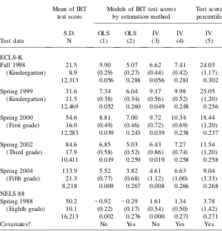
To put the size of these effects into perspective, the coefficients on log family income and mother’s education in IRT test score models are approximately 1.0 and 0.8, respectively, in fall 1998. Therefore, an additional year of age at kinder-garten entry increases average fall kinderkinder-garten reading scores by more than five times as much as raising family income by one log point (a 175 percent increase in income) and by 6.6 times as much as a one-year increase in mother’s education. Table 2 presents estimates of the effects of entrance age on math test scores. IV estimates in Model 5 indicate that an additional year of age at the time of kinder-garten entry is associated with a 24.0 percentile point increase in initial math scores, a 9.0 percentile point increase in math scores in the spring of 2004, and a 3.8 percentile point increase in eighth grade. The initial effects are larger than those for reading scores but show the same pattern of decline from kinder-garten through later grades, with the effect persisting until eighth grade. These estimates are similar in magnitude to Datar’s (2006) findings in kindergarten and first grade and to Bedard and Dhuey’s (2006) findings for third and eighth grade.20
In the IV models presented in Tables 1 and 2, the estimates are generally insen-sitive to the inclusion of a rich set of covariates. Although it is difficult to assess whether predicted entrance age is ‘‘as good as randomly assigned,’’ the similarity of the point estimates in Columns 3 and 4 provides some reassurance about its val-idity as an instrumental variable. As mentioned above, in the Appendix we further assess the validity of our identification strategy in two ways. First, we examine models that use only variation in birth dates or variation in cutoff dates, but not both, as a source of identification. Second, we estimate models that use the discon-tinuity in predicted entrance ages for those born within one month of their state’s cutoff date as the sole source of variation in predicted entrance ages. We find that our baseline results are robust to these alternative specifications, suggesting that these baseline estimates identify a causal effect of entrance age on early educa-tional outcomes.
Our examination of reading and math test scores thus far points to learning prior to kindergarten as the primary source of the relationship between test scores and en-trance age. This relationship is strongest in kindergarten, with nearly all of the effect evident at the very beginning of the fall, before any real learning has taken place in school. Moreover, the performance of older and younger children converge relatively rapidly as children progress through school, which indicates that older children are not able to learn at a faster rate in school. The following section tests the final pre-diction from our model, that entrance age effects are largest among children from rich families.
20. Bedard and Dhuey (2006) use state entrance laws and children’s birthdates to instrument forcurrent
V. Entrance Age, Achievement, and Family Background
A large body of research shows significant differences in early school performance across socioeconomic stratum and racial groups.21Some of these differ-ences are attributable to differdiffer-ences in home environments, parental behaviors, and enrollment in preschool programs. To the extent that high-SES families provide their Table 2
Estimates of the Effect of Kindergarten Entrance Age on Math Test Scores
Mean of IRT test score
Models of IRT test scores by estimation method
Test score percentile
S.D. OLS OLS IV IV IV
Test date N (1) (2) (3) (4) (5)
ECLS-K
Fall 1998 21.5 5.90 5.07 6.62 7.41 24.03
(Kindergarten) 8.9 (0.29) (0.27) (0.44) (0.42) (1.17) 12,313 0.056 0.288 0.056 0.281 0.302
Spring 1999 31.6 7.34 6.04 9.17 9.98 25.05
(Kindergarten) 11.5 (0.38) (0.34) (0.56) (0.52) (1.20) 12,469 0.052 0.260 0.049 0.248 0.256
Spring 2000 54.6 8.81 7.00 9.72 10.34 18.44
(First grade) 16.0 (0.49) (0.46) (0.72) (0.69) (1.20) 12,283 0.039 0.243 0.039 0.238 0.237
Spring 2002 84.6 6.85 5.03 6.43 7.27 11.54
(Third grade) 17.9 (0.58) (0.52) (0.86) (0.74) (1.20) 10,411 0.019 0.259 0.019 0.258 0.258
Spring 2004 113.9 5.52 3.82 4.61 6.63 9.04
(Fifth grade) 21.3 (0.77) (0.68) (1.12) (1.00) (1.33)
8,218 0.009 0.267 0.008 0.266 0.268
NELS:88
Spring 1988 50.2 20.92 20.29 1.61 1.34 3.78
(Eighth grade) 10.1 (0.22) (0.17) (0.54) (0.50) (1.42) 16,213 0.002 0.276 0.000 0.271 0.271
Covariates? No Yes No Yes Yes
Note: The entries for each model are the coefficient, standard error in parentheses, and the regression
r-squared. Standard errors are robust to clustering at the school level. Covariates are described in the text. Grade levels in parentheses reflect the modal grade of students in each survey.
children with higher levels of investment, children’s prekindergarten experience will have a larger effect on test scores among rich children than among poor children. We test this prediction and find evidence that the entrance age effect is substantially larger among children from higher socioeconomic status families, implying that increases in the overall entrance age have the perverse effect of exacerbating socio-economic differences in school performance.
To investigate differences in the effect of kindergarten entrance age on children from different family backgrounds, we begin by classifying children into one of four quar-tiles based on their observable characteristics. Specifically, for ECLS-K children we re-gress the fall kindergarten reading score on all of the exogenous covariates included in Equation 6, such as gender, race and ethnicity, parental income and education, family structure, region, and urbanicity. We then generate a predicted test score for all children in the data based on the coefficients from this model and children’s observable charac-teristics and classify children into quartiles based on this ‘‘family background index.’’ More precisely, this index ranks children according to who is likely to perform well on achievement tests based on their observable characteristics. A similar index is created for children in the NELS:88 based on their eighth grade reading test score.
Table 3 provides descriptive information about children, their families, childcare arrangements, and school performance across the four quartiles in ECLS-K, with Quar-tile 1 representing those with the lowest ‘‘family background index’’ and QuarQuar-tile 4 rep-resenting the highest. Panel A shows that the index is strongly positively correlated with fall kindergarten reading test scores (by construction), maternal education, and family income; and negatively correlated with the probability a child is still in first or second grade in the spring 2002 interview and the probability a child is raised in a one-parent household in the ECLS-K. Although it is not surprising that the variables listed in Panel A are related to the family background index (with the exception of the grade repetition measure, these variables are used to construct the index), the correlations indicate that the index is strongly correlated with familiar measures of family background.
Table 3
Child and Household Characteristics by Family Background Quartile
Panel A: Socioeconomic Characteristics
Quartile 1 22.4 0.174 11.7 19,600 0.403
Quartile 2 25.5 0.084 12.9 35,000 0.274
Quartile 3 28.4 0.048 13.9 50,000 0.157
Quartile 4 33.6 0.037 15.6 80,000 0.036
Overall 27.5 0.088 13.6 45,000 0.214
Panel B: Reading and Related Activities
Parent reads to
Quartile 1 0.365 0.277 0.359 48.6 0.445
Quartile 2 0.411 0.306 0.337 69.6 0.484
Quartile 3 0.448 0.324 0.337 86.4 0.511
Quartile 4 0.602 0.399 0.381 103.5 0.610
Overall 0.461 0.328 0.356 77.3 0.514
Panel C: Primary Childcare Arrangement prior to Kindergarten
Non-Head Start formal care
Quartile 1 0.576 0.334 0.137 0.099 0.078
Quartile 2 0.644 0.167 0.259 0.143 0.109
Quartile 3 0.734 0.057 0.398 0.177 0.117
Quartile 4 0.820 0.013 0.516 0.208 0.086
Overall 0.582 0.139 0.327 0.157 0.098
Note: Family background quartile is defined in the text. Unless noted, data in Panels A and B refer to char-acteristics measured in the fall of kindergarten. Panel C refers to childcare arrangements in the year prior to kindergarten. N¼11,592
library), and these children are also more likely to look at picture books every day. The fraction of children who read (or pretend to read) to themselves is roughly constant across family background quartiles. These correlations between family background and home reading activities during the fall of kindergarten suggest that rich children experience a more enriching home environment that stresses building reading skills and vocabulary.22
Finally, Panel C of Table 3 shows tabulations of children’s primary source of childcare or schooling in the year prior to kindergarten. To varying degrees, formal childcare settings tend to develop young children’s cognitive abilities and the first column of Panel C indicates there are noticeable socioeconomic disparities in for-mal childcare attendance: 57.6 percent of children in the poorest quartile attended some type of formal childcare, while 82.0 percent of children in the richest quartile did so. Data in the second column indicate that about a third of children in the poorest quartile participated in Head Start, accounting for nearly 60 percent of for-mal childcare arrangements among this group.23 The steep gradient in formal childcare enrollment is primarily driven by sharp differences in preschool and prekindergarten enrollment. 51.6 percent of children in the richest quartile were enrolled in preschool or nursery school and an additional 20.8 percent were enrolled in prekindergarten. By contrast, only 23.6 percent of children in the poor-est quartile were enrolled in either type of programs. The three panels in Table 3 indicate clear differences in resources and children’s experiences across the family background spectrum. Next, we turn to direct evidence on differences in the rate of learning prior to kindergarten.
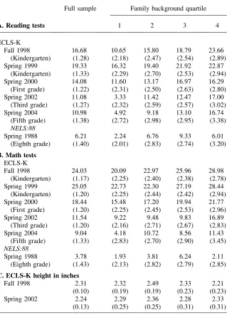
Table 4 explores the variation in the effect of entrance age across the four family background quartiles. Each entry in the table represents an IV estimate ofafrom mod-els of test score percentiles. For both reading and math tests, entrance age effects rise with socioeconomic status. For example, being a year older at kindergarten entry raises average fall 1998 reading scores by 10.65 percentile points among students in the poor-est quartile and by 23.66 percentile points in the richpoor-est quartile; these differences are statistically significant.24The remaining results in Panel A show large differences by quartile in reading score effects through fifth grade, and the results in Panel B show similar effects for math scores. Perhaps more importantly, the benefits of an additional year of entrance age ‘‘fade out’’ relatively quickly for the most disadvantaged children — the effect on reading score percentiles among the upper quartiles in fifth and eighth grade is larger than that for the lowest quartile in third grade. As late as fifth grade, the
22. Lubotsky (2001) and Todd and Wolpin (2006) use the National Longitudinal Survey of Youth-Children to show strong correlations between race or parental resources and a variety of parental behaviors that build children’s skills among families of school-age children.
23. The four righthand columns of Panel C in Table 3 may add up to more than 100 percent because parents could report that their child was in both Head Start and one of the other arrangements. For simplicity, we combine children whose parents report they are in nursery school (1.6 percent of children) with those who report they are in preschool (31.2 percent of children).
Table 4
IV Estimates of Test Score Percentiles and Height, by Family Background Quartile
Full sample Family background quartile
A. Reading tests 1 2 3 4
ECLS-K
Fall 1998 16.68 10.65 15.80 18.79 23.66
(Kindergarten) (1.28) (2.18) (2.47) (2.54) (2.89)
Spring 1999 19.33 16.32 19.40 21.92 22.87
(Kindergarten) (1.33) (2.29) (2.70) (2.53) (2.94)
Spring 2000 14.08 11.60 13.17 16.97 16.29
(First grade) (1.22) (2.31) (2.50) (2.63) (2.80)
Spring 2002 11.08 3.33 11.42 12.47 17.00
(Third grade) (1.27) (2.32) (2.59) (2.57) (3.02)
Spring 2004 10.98 4.92 9.18 13.10 16.74
(Fifth grade) (1.38) (2.72) (2.98) (2.95) (3.38)
NELS:88
Spring 1988 6.21 2.24 6.76 9.33 6.01
(Eighth grade) (1.40) (2.01) (2.83) (2.74) (3.20)
B. Math tests ECLS-K
Fall 1998 24.03 20.09 22.97 25.96 28.98
(Kindergarten) (1.17) (2.25) (2.40) (2.38) (2.78)
Spring 1999 25.05 22.73 22.30 27.19 28.44
(Kindergarten) (1.20) (2.25) (2.44) (2.42) (2.94)
Spring 2000 18.44 15.48 17.20 19.94 21.77
(First grade) (1.20) (2.25) (2.45) (2.53) (2.96)
Spring 2002 11.54 9.22 9.48 9.83 16.89
(Third grade) (1.20) (2.16) (2.71) (2.67) (2.83)
Spring 2004 9.04 4.18 10.72 8.56 11.43
(Fifth grade) (1.33) (2.83) (2.70) (2.90) (3.45)
NELS:88
Spring 1988 3.78 1.93 3.81 6.24 2.11
(Eighth grade) (1.43) (2.13) (2.82) (2.79) (2.85)
C. ECLS-K height in inches
Fall 1998 2.31 2.32 2.49 2.33 2.21
(0.10) (0.19) (0.19) (0.23) (0.23)
Spring 2002 2.24 2.29 2.36 2.28 2.33
(0.13) (0.25) (0.25) (0.31) (0.31)
Notes:
1) All models include covariates. Test scores are measured in percentile units. Standard errors are robust to clustering at the school level.
estimate for the top quartile is larger than the estimate for the bottom quartile for either fall or spring kindergarten. The patterns for math scores are similar but less dramatic. The estimates in Table 4 are consistent with the idea that older children do better in school because they have had more time to build skills prior to entering kindergar-ten. An alternative reason for the association between children’s entrance age and school performance is that age is strongly associated with physical maturity, which may prepare children for the physical and mental rigors of school. Panel C of Table 4 shows IV estimates of the association between a child’s height (as one measure of maturity) and entrance age for the full ECLS-K sample and separately by family back-ground quartile. The results show that each year of age is associated with being 2.3 inches taller in fall 1998 and 2.2 inches taller in spring 2002. More importantly, the next four columns indicate that the relationship between entrance age and height is the same across all four family background groups. The coefficients range from 2.2 to 2.5 inches per year, though the differences across quartiles are not statistically significant in either survey period. We interpret this evidence to mean that physical ma-turity does not play any role in explaining the wide variation in the association between entrance age and educational outcomes across socioeconomic groups. Moreover, since the heterogeneity in Panels A and B is of such a large magnitude, it is unlikely that physical maturity is a driving force in any of the entrance age effects found above.25
VI. The Importance of Entrance Age in Disability
Diagnoses and Grade Retention
As noted above, a number of prior studies have investigated the re-lationship between entrance age and test scores. Much less is known about how en-trance age influences other child outcomes such as the diagnoses of learning disabilities like Attention Deficit/Hyperactivity Disorder (ADD/ADHD) and the suc-cessful progression from one grade to the next. Understanding the determinants of these outcomes is important for a number of reasons. Child mental health is among the most important facets of children’s human capital, a point that the literature on cognitive development has only recently recognized. Currie and Stabile (2006) argue that children who exhibit symptoms of ADD/ADHD, the most common childhood mental health condition, accumulate skills in reading and math at a slower rate than children with common physical health problems, such as asthma. Diagnosis of ADD/ ADHD requires a child to exhibit at least six symptoms by the age of seven and ex-perience these symptoms in at least two settings, such as at home and at school. Teachers are therefore crucial in the process of identifying children who may be in need of professional care. There is also some debate about the accuracy with which child mental health conditions are diagnosed. Since classrooms contain
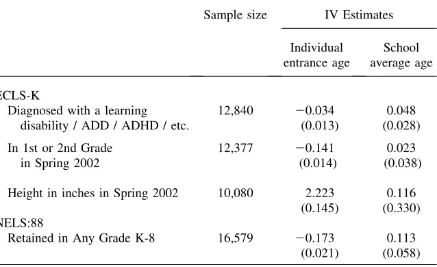
children of varying ages, it is possible that teachers’ perceptions of children who suf-fer from ADD/ADHD are clouded in part by difsuf-ferences in relative age and maturity. Table 5 presents OLS and IV estimates of the effect of entrance age on various measures of learning disability diagnoses and the probability of repeating a grade in school, for both the ECLS-K and NELS:88 full samples and separately by the fam-ily background index described in the previous section. Each survey period, the NCES asks parents of ECLS-K children whether their child had ‘‘been evaluated by a professional in response to {his/her} ability to pay attention or learn.’’ Parents who answered in the affirmative were asked if they received a diagnosis, and what the diagnosis was. The most common diagnoses are dyslexia and related learning disabilities, ADD/ADHD, and developmental delays. We analyze an indicator vari-able that is equal to one if the child was diagnosed in any round of the survey with any type of condition, and we also consider ADD/ADHD diagnoses separately from diagnoses of all other learning disabilities. We present the results for the overall dis-ability measure in the top row of Table 5. The baseline diagnosis rate is 8.8 percent, and the IV estimate in Column 4) indicates that being a year older at the time of kin-dergarten entry reduces the probability of diagnosis by 2.5 percentage points, which represents both the effect of being referred to a specialist and the effect of receiving a positive diagnosis. Note that the OLS and IV estimates are substantially different, im-plying that voluntary delayed entry is positively related to the latent propensity of diagnosis. The next two rows of the table show that ADD/ADHD diagnoses account for the entire entrance age-learning disability gradient, with an additional year of age at entry decreasing the probability of an ADD/ADHD diagnosis by 67 percent (¼
-0.029 / 0.043) relative to the baseline diagnosis rate. Disabilities other than ADD/ ADHD have essentially no relationship with entrance age.
A large literature has documented the association between ADD and ADHD diag-noses and a child’s ‘‘season of birth.’’26The results of Table 5 are insensitive to the inclusion of controls for season or month of birth, implying that it is not season of birth, per se, but a child’s exogenously determined age of entry into kindergarten that influences ADD/ADHD diagnoses.27This interpretation may confirm the notion that ADD/ADHD diagnoses are more subjective than diagnoses of mental retardation and learning disabilities such as dyslexia. Some diagnoses may simply reflect a lack of emotional maturity among young kindergarten entrants; alternatively, the oldest children in a class may be under-diagnosed because their disabilities are masked in comparison to the behavior of younger classmates. Distinguishing between these hypotheses is beyond the scope of this paper, but the results suggest that future re-search into the mechanisms of ADD and ADHD diagnoses may prove fruitful.
The bottom rows of Table 5 present estimates of the effect of entrance age on the probability of repeating a grade in school. The ECLS-K grade repetition measure is equal to one for children who are in first or second grade in the spring 2002 interview, when ontrack children should be in third grade, and the NELS:88 measure is equal to one if a student reported having to repeat any grade before 1988. In both data sets, IV estimates show that children who enter at older ages are significantly less likely to
26. See, for example, Mick, Biederman, and Faraone (1996).
Table 5
The Effect of Kindergarten Entrance Age on Grade Retention and Learning Disabilities in the Full NELS:88 and ECLS-K Samples and by Family Background Quartile
Dependent Variable Mean
N
Family background quartile
OLS OLS IV IV
(1) (2) (3) (4) 1 2 3 4
ECLS-K
Diagnosis of learning disability/ADD/ADHD/etc.
0.088 0.008 0.005 20.026 20.025 20.038 20.006 20.053 20.012
12,860 (0.008) (0.009) (0.011) (0.012) (0.026) (0.028) (0.030) (0.022)
[20.332] [20.056] [20.698] [20.190]
Diagnosis of ADD/ADHD 0.043 20.004 20.011 20.021 20.029 20.040 20.008 20.042 20.034
12,860 (0.006) (0.006) (0.007) (0.009) (0.020) 2(0.049) (0.021) (0.015)
[20.808] [20.132] [20.974] [21.133] Diagnosis of non-ADD/ADHD
learning disability
0.045 0.012 0.014 20.004 0.001 0.000 0.003 20.009 0.018
12,860 (0.005) (0.005) (0.007) (0.008) (0.016) (0.018) (0.017) (0.015)
[20.004] [0.077] [20.311] [0.653]
In 1st or 2nd grade in Spring, 2002
0.088 20.112 20.112 20.116 20.131 20.214 20.135 20.087 20.120
10,431 (0.010) (0.011) (0.013) (0.015) (0.038) (0.029) (0.026) (0.026)
[21.232] [21.609] [21.808] [23.269] NELS:88
Retained in any grade K-8
0.214 20.078 20.092 20.171 20.155 20.185 20.187 20.108 20.112
16,585 (0.011) (0.011) (0.019) (0.022) (0.046) (0.045) (0.039) (0.032)
[20.497] [21.273] [20.734] [21.332]
Covariates? No Yes No Yes Yes Yes Yes Yes
Note: Entries include the coefficient and standard error for each model. Terms in [brackets] are the ratio of the coefficient to the probability of each outcome in each quartile. Standard errors are robust to clustering at the school level.
Covariates are described in the text.
The
Journal
of
Human
repeat a grade. Our preferred estimates in Column 4 are -0.131 for ECLS-K and -0.155 in NELS:88, both of which are strikingly large relative to the sample probabilities of 0.088 and 0.214, respectively. As was the case for math and reading test scores, in the Appendix we find that the full-sample results of Table 5 are insensitive to alternative specifications such as a discrete version of a regression discontinuity design.
In the four rightmost columns of Table 5, we show separate estimates for each family background quartile. The baseline averages vary considerably across the quar-tiles for all five outcomes, so below the coefficients and standard errors we display the ratio of the coefficient to the baseline rate for each cell (in brackets). These mod-els point to larger grade retention effects of entrance age relative to the baseline rate for richer children. For example, an additional year of age at kindergarten entry low-ers the probability of grade retention by 21.4 percentage points among the poorest quartile in the ECLS-K. This group had a baseline retention rate of 17.4 percent, so the ratio of the effect size to the baseline rate is -1.23. Among the richest quartile, the point estimate is 12.0, which is 3.27 times their baseline retention rate of 3.7 per-cent. We find no pattern across quartiles for any of the learning disability diagnoses. Although there appear to be differential effects on grade repetition across the four family background quartiles, this pattern does not shed much light on whether the association is due to learning before or after school entry. Unlike test scores, out-comes such as grade repetition and ADD/ADHD diagnoses confound skills learned prior to school entry and during kindergarten (and later grades) because they are not measured at a point in time immediately after kindergarten entry. Regardless of the reason, younger entrants are apparently more likely to suffer from shortcomings in skills or maturity by the end of kindergarten, and these deficits lead teachers and parents to suggest professional evaluation and grade repetition as remedies. In the following section, we pursue an additional strategy that will shed light on the mech-anism underlying the ADD/ADHD and grade repetition effects.
VII. Peer Effects in Kindergarten Entrance Age – Is
It Relative or Absolute Age That Matters?
We next investigate whether entrance age laws affect outcomes be-cause they influence an individual child’s age, bebe-cause they influence the average age of a class (and hence a student’s age relative to the class average), or both. There are several reasons why the average age of a class may influence student outcomes. First, an older class may have fewer disruptions or allow a teacher to focus on more advanced material.28Second, the achievement or behavior of older students may have a positive spillover effect on younger students. Alternatively, a child’s own age may matter only through its effect on the child’s location in the classroom age distribution. A five year old may struggle if he is the youngest in a class with a cur-riculum targeted at older students, but the same child may do well if placed in a class with a younger average age.
The distinction between the impacts of a child’s absolute entrance age and his age relative to classmates is important for the design of education policy. If entrance age gra-dients are solely due to the relative age mechanism, changes in entry cutoffs will simply change which children are the youngest in the class and which are the oldest, without any aggregate benefits for skill attainment. These policy changes would involve real costs, though, as some children would be forced to remain out of school an extra year. To model the independent effect of classmates’ average entrance age, we augment Equation 6 withEAs;2i, the average entrance age in schoolsover all sampled chil-dren from a school except childi, andXs;2i, a vector of the school average covariates.
The model of child outcomes thus becomes
Yis¼u1EAis+u2EAs;2i+Xisg+Xs;2iu+eis:
ð8Þ
Unobserved determinants of outcomes are likely to influence individual entrance ages and school averages, so we instrument both measures with predicted individ-ual entrance age and the school average if all students perfectly complied with statewide kindergarten entrance policies. Identification of bothf1andf2is possi-ble because variation in absolute age at entry depends on entrance cutoffs and in-dividual birthdays, although variation in school averages is generated by variation in average birth dates across schools and variation across schools in the entrance age cutoffs.29In practice, almost all of the variation in predicted school average entrance ages is due to variation across states in entry cutoff dates, so the estimates of f1 andf2 are largely insensitive to fixing average birth dates across schools within a state.
Before proceeding, we note that the statistical model in Equation 8 also captures the idea that peers matter because a child’s performance is influenced by his or her age relative to the class average age. To see this, note that the model given by:
Yis¼d1EAis+d2ðEAis2EAs;2iÞ+Xisg+Xs;2iu+eis
ð9Þ
is equivalent to that in Model 8, withu1¼d1+d2andu2¼-d2. Put differently, with-out putting additional structure on the data, we cannot decipher whether peers matter because of direct spillovers from older students to younger ones (or vice versa), or be-cause teachers design curriculums to best teach the average child. Thus, we proceed with estimates of Equation 8 but note that a positive effect of the school average en-trance age (f2) corresponds to a negative effect of a child’s age relative to the school average.
Table 6 presents IV estimates of Equation 8 for math and reading test scores in ECLS-K and NELS:88. The above discussion implies that the class average en-trance age will not be related to fall kindergarten test scores, but may affect later
Reading Tests
Sample Size
IV Estimates Math Tests Sample Size
IV Estimates
Individual entrance age
School average age
Individual entrance age
School average age
ECLS-K ECLS-K
Fall 1998 11,576 17.08 5.28 Fall 1998 12295 24.73 0.98
(1.25) (3.36) (1.17) (2.78)
Spring 1999 11,957 18.66 9.33 Spring 1999 12451 24.33 7.47
(1.22) (3.84) (1.16) (3.09)
Spring 2000 12,032 13.66 5.55 Spring 2000 12269 17.95 5.59
(1.15) (3.58) (1.14) (3.19)
Spring 2002 10,323 10.87 3.01 Spring 2002 10398 10.97 5.71
(1.28) (2.99) (1.20) (3.34)
Spring 2004 8,199 10.55 4.67 Spring 2004 8207 9.52 20.59
(1.44) (3.22) (1.42) (3.76)
NELS:88 NELS:88
Spring 1988 16,209 5.72 3.11 Spring 1988 16206 3.47 2.77 (Eighth grade) (1.41) (3.83) (Eighth grade) (1.33) (4.17)
Note: All models control for the individual covariates described in the text and school averages of those covariates. Standard errors (in parentheses) are robust to clustering at the school level.
Elder
and
Lubotsky