Darius Lakdawalla
Tomas Philipson
a b s t r a c t
We use panel data from the National Longitudinal Survey of Youth to investigate on-the-job exercise and weight. For male workers, job-related exercise has causal effects on weight, but for female workers, the effects seem primarily selective. A man who spends 18 years in the most physical fitness-demanding occupation is about 25 pounds (14 percent) lighter than his peer in the least demanding occupation. These effects are strongest for the heaviest quartile of men. Conversely, a male worker spending 18 years in the most strength-demanding occupation is about 28 pounds (15 percent) heavier than his counterpart in the least demanding job.
I. Introduction
The well-documented rise in obesity has attracted a great deal of at-tention and generated concern (Flegal et al. 1998; Flegal et al. 2002; Mokdad et al. 2000; Mokdad et al. 1999; Seidell and Deerenberg 1994; VanItallie 1996). From 1976 to 2001, the rate of obesity among U.S. adults more than doubled, from just below 9 percent to more than 20 percent (Philipson and Lakdawalla 2006).1 While the most rapid growth in weight has occurred among those who are the most
Darius Lakdawalla is a senior economist at the RAND Corporation. Tomas Philipson is a professor of economics at the University of Chicago. The authors wish to thank seminar participants at AEI, The University of Chicago, Columbia University, Harvard University, MIT, The University of Minnesota, The University of Toronto, UCLA, Yale University, the 2001 American Economic Association Meetings, the 2001 Population Association of America Meetings, the 12th Annual Health Economics Conference, Gary Becker, Shankha Chakraborty, Mark Duggan, Michael Grossman, Bob Kaestner, John Mullahy, Casey Mulligan, Richard Posner, and Chris Ruhm. Erin Krupka provided excellent research assistance. Darius Lakdawalla thanks the RAND Institute for Civil Justice for financial support. The data used in this article can be obtained beginning August 2007 through July 2010 from Darius Lakdawalla, RAND Corporation, 1776 Main Street, Santa Monica, CA 90407, darius@rand.org.
[Submitted July 2005; accepted March 2006]
ISSN 022-166X E-ISSN 1548-8004Ó2007 by the Board of Regents of the University of Wisconsin System
T H E J O U R NA L O F H U M A N R E S O U R C E S d X L I I d 1
overweight, weight growth has been observed throughout the weight distribution. Figure 1 plots the 1976 and 2001 distributions of Body Mass Index (BMI), a measure of height-adjusted weight, for US adults aged 18 to 65. Over this 25-year period, the 25th, 50th, and 75th percentile values for BMI increased by 1.8, 2.2, and 2.8 units, respectively. The adverse health consequences of these trends are well understood. Obesity and overweight are substantial risk factors for most of the high-prevalence, high-mortality diseases, including heart disease, cancer, and diabetes (Tuomilehto et al. 2001, Wolf and Colditz 1998). Conversely, a healthy level of muscle mass has a protective effect on health (see particularly, Kell et al. 2001).
Both the rapid growth in obesity and the associated concern for public health are relatively new phenomena, but weight itself has been rising for more than a century. The period 1864–1991 witnessed a greater than 15 percent increase in height-adjusted weight for middle-aged adult males in the United States (Costa and Steckel 1995). While rising food consumption has been emphasized as a contributor to rising weights (Putnam 2000; Putnam and Allshouse 1999; Putnam et al. 2002), the histor-ical record demonstrates that declining physhistor-ical activity has played an undeniable role. From 1944 to 1961, height-adjusted weight increased by about as much as it did during the comparably long 1976 to 1994 ‘‘obesity boom’’ period, even though Figure 1
Change in the Body Mass Index (BMI) Distribution among U.S. Adults Aged 18–65, 1976–2001.
the supply of calories remained constant or fell.2This historical perspective suggests the importance of understanding the role played by exercise in weight determination, but it also points specifically to the potential role ofjob-related exercise: The rise in developed-country obesity may have been driven in part by economic progress, which not only lowers the price of calories through agricultural innovation but also makes work more sedentary in the shift to a more skilled labor force (Philipson and Posner 1999). Historically, workers were paid to exercise through manual labor. Be-cause on-the-job exercise has become less common, many workers today must pay to exercise, mainly in terms of foregone leisure.
On-the-job exercise is likely to have significant impacts on weight, because even small daily changes in physical activity have large cumulative effects. For example, Hill et al. (2003) argue that walking an additional 15 minutes per day would prevent weight gain in most of the U.S. population. Moreover, according to our data, occu-pations vary quite widely in the physical demands they place on workers. Therefore, differences in occupation may induce substantial variation in weight.
Clearly, however, differences in weight depend on differences both in jobs and in the workers who choose to enter them. This makes it important to separate the causal effects of a job from weight-based selection into jobs. Our empirical analysis sug-gests that causal effects seem dominant for male workers, but that selection seems important for females. Remaining in the most fitness-demanding occupations for 18 years leaves a male worker 3.5 BMI units lighter than if he had spent that time in one of the least demanding occupations. This is approximately equal to 11.2 kg of weight loss (24.7 pounds, or 14 percent of body weight) for a man of average height. Quantile regression analysis suggests that these weight-loss effects are con-centrated in the top decile or quartile of the BMI distribution, where individuals are obese or significantly overweight, and thus likely to benefit from weight reduc-tion. On the other hand, jobs with muscular requirements can encourage weight gain in the form of muscle building. Spending 18 years in an occupation with the most physical strength demands raises BMI by about four units for males, compared to an occupation at the bottom of the strength distribution. This is about 12.8 kg (28.2 pounds, or 15 percent) of weight gain. There is no detectable evidence that se-lection plays a quantitatively significant role in these effects. Female workers, how-ever, seem to select into occupations according to their weight. From the very first year of labor force participation, the weight of female workers differs systematically across occupational types. Moreover, these baseline differences in weight actually
diminishwith exposure to the labor force. In light of both these facts, we cannot
identify an effect of occupation on weight that seems plausibly causal for females. The paper may be briefly outlined as follows. In Section II, we provide some back-ground on occupation and physical activity in the United States, using data from the Dictionary of Occupational Titles. Section III presents the analysis of panel data on occupation and weight for male and female workers from the National Longitudinal
Survey of Youth (NLSY). In Section IV, we estimate the relationship between occu-pational characteristics and body weight, and then investigate the degree to which these effects are causal. Section V concludes.
Our paper relates to the significant economics literature on the relationship be-tween health and labor supply (see Bound et al. 1998; Smith and Willis 1999). In addition, Case and Deaton (2003) have recently studied the impact of occupation on health throughout the life-cycle. They argue that low-paid, manual work damages self-assessed health more than highly paid, skilled work. We focus on a different causal mechanism from labor supply to health—namely body weight—that may have quite different and possibly more complicated distributional implications. This study also relates to the emerging economics literature focused on weight. This lit-erature has stressed technological change in the production of food and the incentive to exercise as key determinants of historical growth in weight (Chou et al. 2004; Cut-ler et al. 2003; Lakdawalla and Philipson 2002; Lakdawalla et al. 2005). Other rel-evant research has examined the links among appearance, weight, and wages (Averett and Korenman 1996; Biddle and Hamermesh 1998; Cawley 2004; Hamermesh and Biddle 1994). So far, however, economists have spent less effort understanding the effects of job-related exercise on weight and the implications of labor supply for the overall weight distribution in a population.3
II. Physical Activity, Occupation, and Weight
A. Measuring Physical Activity
We are interested in the empirical contribution of occupational exercise to the main-tenance of a healthy weight. However, the concept of ‘‘healthy weight’’ is complex, because different kinds of weight gain have different impacts on health. People gain weight because they acquire muscle, and they also gain weight when they lead sed-entary lives that promote fatness. Weight gain benefits health in the first case but harms it in the second. Although it would be preferable to have multidimensional measures of weight, these are not readily available in data sets with detailed data on occupation.4Instead, we use multidimensional measures of job-related exercise in an attempt to separate different kinds of weight gain. Throughout the analysis, we distinguish between physical demands that promote agility and fitness, and strength requirements that encourage muscle gain. We call the former ‘‘fitness demands’’ and the latter ‘‘strength demands.’’ This is similar to the distinction drawn in the medical literature, which distinguishes between muscle-building exercise, and exercise that increases endurance and agility (see Sinaki et al. 2004). The former is empirically associated with weight loss (see Sykes et al. 2004), while the latter is associated with weight gain (see Abe et al. 2003).
3. There has been some research in medicine and public health linking job-related activity to physical fit-ness (see for example, Tammelin et al. 2002). Most such studies have focused on specialized samples and have not been interested in distinguishing between causality and selection.
The distinction between fitness-promoting and strength-building exercise is also relevant for understanding the health impacts of exercise and weight. A wide variety of studies find that weight-reducing exercise in our sense of fitness demands helps prevent chronic disease and protect health. Randomized controlled trials suggest that such physical activity helps control blood pressure (Appel et al. 2003), prevents the onset of diabetes (Gin et al. 2003; Knowler et al. 2002), controls diabetes-related morbidity (Maiorana et al. 2002), prevents coronary heart disease (Thompson and Lim 2003), and improves functional capacity (Maiorana et al. 2001). An emerging literature also suggests that muscle-building resistance exercise (as in strength demands) benefits health (see Katzmarzyk and Craig 2002; Kell et al. 2001).
B. Data on Occupational Characteristics
At the heart of this and the subsequent analysis is our measurement of job-related exercise. The Dictionary of Occupational Titles (DOT), compiled and published by the Department of Labor, contains a wealth of information about the characteris-tics of different occupations in the United States. Department of Labor analysts con-struct detailed occupational characteristics, based on fieldwork and their expert knowledge. First published in 1939, the DOT has been updated over time. We use the revised fourth edition, first published in 1991, and containing the result of updates by Department of Labor analysts from 1981 to 1991, the period during which the NLSY cohort entered the labor force.
The DOT is, literally, a dictionary of all occupations in the United States. Each occupational definition lists a title for the occupation, as well as a description of the occupationÕs skill requirements and demands. Among these listed demands are the jobÕs physical demands, which we use in this study.
For each occupation,5the DOT reports on 20 physical demands. The first is a measure of strength demands, which we use directly. This is an ordinal scale from one to five, corresponding to: sedentary, light, medium, heavy, and very heavy. Since this is an ordinal measure, whose changes do not have a clear quantitative interpretation, we con-vert it to a percentile. For each worker, we compute his or her percentile in the sex-specific distribution of strength ratings, using pooled data over the 1982–2000 NLSY waves. This we call the ‘‘strength demands percentile’’ throughout the text. Later, we discuss the interpretation and testing of models that include a percentile based on an ordinal measure.
Of the remaining 19 physical demands, seven are related to physical agility or fit-ness.6We use these to measure the ‘‘fitness’’ demands of a job. Specifically, the DOT reports on which of the following physical tasks is required by the occupation: climb-ing, balancclimb-ing, stoopclimb-ing, kneelclimb-ing, crouchclimb-ing, crawlclimb-ing, and reaching. We use the sum of the demands present as an index of ‘‘fitness demands.’’ Each occupation can be associated with anywhere from zero to seven fitness demands.
musculoskeletal breakdowns that affect health and possibly also BMI.7 Therefore, our results apply to the whole complex of characteristics associated with physically demanding (or less demanding) jobs.
Figure 2 shows the distribution, by gender, of strength and fitness demands.8By way of example, some common occupations with a strength demand rating of ‘‘sed-entary’’ include accountants, managers and administrators, tabulation machine oper-ators, and photographic process workers. Some common occupations with a strength demand rating of medium include carpenters, automobile body repairmen, and plumbers. The only occupations rated heavy are carpet installers, plumberÕs appren-tices, and garbage collectors. For fitness demands, a few representative sedentary occupations with no measured fitness demands are labor relations workers, and insur-ance agents/brokers/underwriters. A set of active occupations with three or four demands are marine scientists, athletic coaches, teachers, urban/regional planners, carpenters, and construction laborers.
A casual look at the occupations above paints a rich and complex picture of how the physical attributes of jobs vary. Although one might think that physical activity is always higher in less skilled jobs, this is not always the case. Of course, the examples do make clear that education plays a role, and it seems to play even more of a role for strength demands than for fitness demands. Among working men in the 2000 NLSY, college grad-uates were on average 39 percentile points below high school dropouts in the strength rating distribution, and had 1.2 fewer fitness demands than high school dropouts. Perhaps for this reason, fitness demands and strength requirements covary positively, with a cor-relation coefficient around 0.5 to 0.6. Therefore, quite a few jobs promote both healthy weight-reduction and muscle-building, while others do the opposite.
III. The Data on Occupation on Weight
The earlier analysis provided suggestive preliminary evidence that exposure to an occupation has cumulative effects on the weight of male workers. To explore this further, we employ panel data on male workers from the National Longitudinal Survey of Youth (NLSY).
A. NLSY Data
We couple the Revised Fourth Edition of the DOT (released in 1991) with NLSY data from 1982 to 2000. The NLSY started in 1979 with a cohort of 12,686 people aged 14 to 22. It asked respondents about their weight in 1982, 1985, 1986, 1988, 1989, 1990, 1992, 1993, 1994, 1996, 1998, and 2000.9It also asked respondents about their height in 1982 and 1985. Because all respondents were older than 21 in 1985, we take the 1985 height to be the respondentÕs height for the remaining survey years. In addition to questions about height and weight, the NLSY asked respondents about their race, 7. Case and Deaton (2003) investigate the adverse impacts of strenuous jobs on health.
Figure 2
Distribution of Occupational Characteristics in NLSY, 1982-2000.
Source: NLSY, 1982-2000.
walla
and
Philipson
sex, marital status, age, and the individualÕs occupation in terms of the 1970 Census clas-sification. We use the latter variable to link the NLSY to the DOT data on occupational characteristics. The NLSY also asks detailed income questions. We use data on wages earned, the primary source of earned income. Our sample includes all workers for 12 waves during which the NLSY collected data on weight.
In the NLSY, weights are self-reported. Since there tends to be systematic bias in the reporting of weight—women tend to under-report their weight, while light men over-report and heavy men under-report—we use the method of Cawley (2000) to correct for it. We use data from Wave III of the NHANES, which was collected from 1988 to 1994. The NHANES is an individual-level data set containing both self-reported weight and height, and measured weight and height, for each individual in the sample.10We regress self-reported weight and its square on actual weight in the NHANES. This regression is run separately for white males, white females, non-white males, and nonnon-white females. TheR-Squared for all these regressions is over 90 percent, indicating that the quadratic function fits the data quite well. As men-tioned earlier, nearly all women tend to under-report their weight; the under-reporting is somewhat greater for nonwhite women than for white women. The reporting pat-terns of men, on the other hand, differ more by weight. Lighter men, who report weight under 100 Kg, tend to say they are heavier than they really are, while heavier men tend to understate their weight. Using the estimated relationship from the NHANES data, we predict actual weight in the NLSY from the self-reported weight data.11All our analysis is performed using this constructed series. Correcting for reporting error improves the fit of our regressions very slightly, but it does not appre-ciably change the quantitative (and certainly not the qualitative) results.12
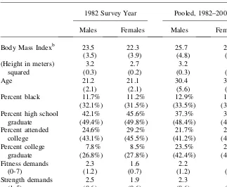
The NLSY data are summarized in Table 1. We report summary statistics for 1982, the first year of our analysis, as well as for the pooled time-series. In 1982, mean BMI for NLSY men and women was in the normal range (20–25). In the overall pooled time-series, however, mean BMI is in the overweight range (25+) for men, and nearly overweight for women. The table also shows the square of height in meters for the average man and woman. This number provides a simple way of trans-lating BMI effects into weight effects: Multiplying this number by an estimated change in BMI yields the equivalent weight change in kilograms for the average person. Finally, the table shows mean fitness demands, and the mean strength rating, using the five-point scale discussed earlier. Recall that in our regression analysis, we use the actual number of fitness demands as a regressor, but use the percentile in the overall pooled sex-specific strength rating distribution (1982–2000).
B. Validating the Occupation Data
Our measures of occupational characteristics come from an external source that is linked to survey data containing measures of respondentsÕweight. The external measures have 10. Unfortunately, the NHANES cannot be used to investigate occupation and weight, because it uses a very coarse system of occupational classification.
11. This general strategy for correcting reporting error is presented in Lee and Sepanski (1995), and Bound et al. (1999). Cawley (2000) applies this strategy to predicting young womenÕs weight.
the advantage of being easily linked to any survey year, but this raises the question of whether our DOT data accurately measure the characteristics of respondentsÕactual occupations. To assess the accuracy of the DOT measures, we analyze self-reported data on occupational characteristics from the 1998–2000 NLSY waves, and see how well the DOT data are associated with these self-reported job characteristics.
Starting in 1998, the NLSY administered a health supplement to its respondents at or above age 40. Part of this supplement included questions about physical activity on the job. The first question is ‘‘How often does your job require lots of physical effort?’’ Respondents must choose one of the following four answers: All or most of the time; most of the time; some of the time; none or almost none of the time. Additionally, NLSY respondents are shown a list of physical demands and asked which, if any, they encounter in their job. Four of these demands are directly related to the strength rating and physical demands measures that we use: (1) lift or carry weights heavier than ten pounds; (2) lift or carry weights lighter than ten pounds; (3) use stairs and inclines; (4) stoop, kneel, or crouch; or (5) reach for supplies, mate-rials, etc. The first (and possibly the second) corresponds to the strength requirements Table 1
Summary Statistics for NLSY
1982 Survey Year Pooled, 1982–2000a
Males Females Males Females
Note: Standard deviations appear in parentheses. Sample limited to workers 18 and older. a. Includes 1982, 1985–86, 1988–90, 1992–94, 1996, 1998, and 2000.
of a job. The last three directly correspond to the fitness demands we are measur-ing—climbing, stooping/kneeling/crouching, or reaching.
Given these self-reported characteristics, we estimate models of the following form:
Charit¼b0 +b1FitDmdit +b2StrengthPctit +b3Demogit+eit ð1Þ
The dependent variable is one of the self-reported job characteristics from the NLSY. The variable FitDmd represents the DOT measure of fitness demands, while
StrengthPctrepresents the percentile in the DOT strength rating distribution, which
is used as an explanatory variable in our analyses. Finally,Demogis a vector of demo-graphic characteristics used in all our analyses: age, age-squared, education dummies (high school graduate, college attendee, and college graduate), survey year dummies, black, hispanic, and decile in the annual earnings distribution. We estimate OLS models for each of the binary job characteristics, and an ordered probit for the one multinomial characteristic (how often does your job require lots of physical effort?). The marginal effects onFitDmdandStrengthPctassociated with each modeled job characteristic are given in Table 2. The table, which shows results for male workers, shows that the DOT measures are reasonably well-correlated with self-reported job characteristics.
Both fitness demands and strength demand ratings are correlated with the general question about physical effort on the job. Not surprisingly, the DOT fitness demands measure is most strongly correlated with the questions about climbing, stooping, and reaching, all of which are fitness demands that the DOT considers. Workers in occu-pations demanding more strength according to the DOT are more likely to report having to lift objects heavier than 10 pounds. A 50 percentile point movement in the strength rating distribution increases this probability by nine percentage points. The results for female workers are somewhat different. For females, the strength rating variable does seem lined up with self-reported weight-lifting requirements: a ten percentile jump in the DOT strength rating distribution increases the probability of lifting weights more than 10 pounds by 4.4 percentage points. Strength ratings are also highly correlated with a womanÕs report that her job requires lots of physical effort. However, the DOT fitness demands measure seems poorly correlated: In-creased DOT fitness demands are positively correlated with climbing and walking around, negatively correlated with lifting light weights, but uncorrelated with all other measures, including the general characterization of physical effort required on the job. Particularly striking is the lack of correlation with stooping, or reaching, both of which are components of the DOT measure for fitness demands. This sug-gests that the fitness demands measure is better for male workers than female work-ers, although the strength rating measure seems adequate for both males and females. This interpretation is quite consistent with all our subsequent analyses using these measures: The fitness demands measure for female workers is the only DOT measure not consistently correlated with weight.
IV. Occupation and Weight Growth Over Time
Table 2
DOT Job Characteristics compared to self-reported job characteristics
Independent Variables
Fitness Demands (0–7)
Strength Demands (Percentile)
Dependent Variable Mean
Marginal Effect
Standard Error
Marginal Effect
Standard Error How often does your job require lots of physical effort?
All or most of the time 26.3% 1.4%* 0.8% 0.36%** 0.03%
Most of the time 18.9% 0.9%* 0.5% 0.23%** 0.02%
Some of the time 29.9% – 0.5%* 0.3% – 0.12%** 0.02% None or almost none of
the timea
24.8% – 1.8% n/a – 0.47% n/a
Does your job require you to lift weights more than ten pounds?
Yes 71.1% 2.3%* 1.3% 0.18%* 0.06%
Noa 28.9% – 2.3% n/a – 0.18% n/a
Does your job require you to climb stairs and inclines?
Yes 54.0% 13.2%** 1.5% – 0.33%** 0.07%
Noa 46.0% – 13.2% n/a 0.33% n/a
Does your job require you to stoop, kneel, or crouch?
Yes 70.5% 6.2%** 1.3% 0.08% 0.06%
Noa 29.5% – 6.2% n/a – 0.08% n/a
Does your job require you to reach for supplies, materials, etc.?
Yes 76.5% 5.1%** 1.2% – 0.10% 0.06%
Noa 23.5% – 5.1% n/a 0.10% n/a
Does your job require you to lift weights less than 10 pounds?
Yes 73.9% 3.3%** 1.2% 0.08% 0.06%
Noa 26.1% – 3.3% n/a – 0.08% n/a
Does your job require you to walk around?
Yes 89.0% 3.6%** 1.0% – 0.15%** 0.04%
Noa 11.1% – 3.6% n/a 0.15% n/a
*Significant at 10 percent; **significant at 5 percent
individualÕs lifetime exposure to physically demanding jobs. A simple approach would be to estimate models that included separate variables that encapsulated the indi-vidualÕs entire history of strength and fitness demands, using (at the extreme) one re-gressor for each wave of data available. Less extreme versions would pool over several waves. We have found that using just two to three regressors for each of the occupational characteristics produces results that are difficult to interpret; the set of occupation variables is highly significant jointly, but the coefficients on individual regressors are unstable and not consistently significant. Therefore, we need a more parsimonious way of summarizing an individualÕs work history.
An individual has experienced adistributionof job characteristics over time. The simplest way to characterize a distribution is with its mean. Therefore, we construct the individualÕs mean fitness demands, and mean strength percentile, starting with 1982. The mean of fitness demands should be interpreted as the mean number of fit-ness demands faced by the worker during his tenure in the labor force observed up to that point.13For example, in 2000, the mean fitness demands span 18 years of data; in 1988, they span six years, and so on. To be precise, in each survey yearT, we have mean fitness demands for individuali:
MeanFitnessiT ¼
1
T
XT
t= 1
FitDmdit
ð2Þ
The mean strength percentile measure is constructed similarly by averaging the per-centile in the strength rating distribution for each respondent. This variable should be interpreted as an individualÕs expected position in the strength rating distribution over his lifetime to date.
While it is simple and attractive to characterize a distribution using only its mean, this may not be complete. We are assuming, for instance, that an individual who spends half his time in a job with two fitness demands and the other half in a job with one de-mand is similar to someone who has faced 1.5 dede-mands throughout. To assess the val-idity of this assumption, and more generally the valval-idity of modeling the distribution of characteristics using only the mean, we tested whether the standard deviations of the two occupational measures had any explanatory power. While the mean experience of an individual proved highly and consistently significant in a variety of specifications, the standard deviation of his historical experience was always insignificant and added no explanatory power, suggesting that the use of mean characteristics alone serves as a simple and useful approximation for the lifetime distribution of job characteristics.
A. Results
Using the mean occupation characteristics described above, we estimate models of the following form for each year of dataT:14
BMIiT =g0+g1MeanFitnessiT+g2MeanStrengthiT+g3DemogiT+eiT ð3Þ
13. We experimented with various weighting schemes for these averages and found the results to be insen-sitive, so we present an unweighted average, which has the simplest interpretation.
Note that each regression is run for a single year in this specification.DemogiT is a vector of demographic characteristics including age, age-squared, dummies for edu-cation group, black, Hispanic, dummies for decile in the annual earnings distribution, and dummies for single-digit 1970 Census occupation category.
Table 3 shows the regression results for year-by-year analyses of weight and life-time occupational characteristics. Early in the cohortÕs life cycle, there is no signif-icant difference in weight across occupations. Signifsignif-icant differences emerge for longer work histories. This suggests that the effects of work take time to accumulate. Remaining in the most fitness-demanding occupations for 18 years leaves a male worker 3.5 BMI units lighter than a demographically similar individual who spent that time in one of the least demanding occupations.15For a man of average height, this is equivalent to losing 11.2 kg of weight (24.7 pounds, or 14 percent of body weight). Moving up one standard deviation in the fitness demands distribution for male workers (gaining 1.2 fitness demands) lowers BMI by about 0.7 units; this is 2.25 kg (5.0 pounds, or 3 percent of body weight) for the average man. On the other hand, spending 18 years in an occupation 25 percentile points higher in the strength demand distribution raises BMI by about one unit for male workers.
Another result of note for male workers is the nonmonotonic effect of schooling: High school graduates have higher BMI than high school dropouts (the excluded group), but BMI seems to decline thereafter. This is consistent with earlier research documenting a nonmonotonic effect of income and socioeconomic status on male BMI (Lakdawalla and Philipson 2002).
For female workers, the effects of being in a strength-demanding occupation are quantitatively similar, although they seem present at the outset of working life. Since they are present before exposure to the effects of occupation, these effects are more likely to be selective than causal, as we discuss later. Moreover, there seems to be little systematic relationship between fitness demands and BMI for female workers. This could be due to the poor correlation of DOT fitness demands with the actual fitness demands of female workers, as discussed in Section B. For both variables, it is difficult to document evidence of plausibly causal effects for female workers.
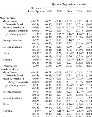
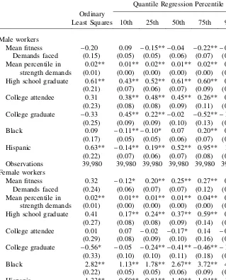
All these effects are evaluated at the mean, but weight gain or loss have very dif-ferent effects at difdif-ferent locations in the BMI distribution. Therefore, we would like to know how these effects vary across the BMI distribution. To do this, we estimate quantile regressions at the 10th, 25th, 50th, 75th, and 90th percentiles of the BMI distribution. Table 4 shows these results for the 2000 NLSY survey year. The table suggests that the effects of strength demands cut across the entire BMI distribution, but that fitness demands seem to matter only for the obese (90th percentile of the BMI distribution). This probably overstates the case a bit, because quantile regres-sions on a single year do not have enough power to rule out smaller negative effects. To address this problem, we conserve statistical power by running pooled quantile models shown in Table 5. Because the coefficients are averaged across occupational histories of different length, they are not directly interpretable. Therefore, we focus on their signs and relative magnitudes. For male workers, fitness demands have the biggest negative effects at the 75th percentile and 90th percentile, with the largest effect at the 90th percentile. There is also a modest significant negative effect at
Table 3
Dynamic Effects of Occupation in the NLSY
1982 1985 1986 1988 1989 1990 1992 1993 1994 1996 1998 2000
Male workers
Mean fitness – 0.01 – 0.02 – 0.06 – 0.01 – 0.03 – 0.08 – 0.49** – 0.39* – 0.46* – 0.50* – 0.31 – 0.57* Demands faced (0.11) (0.14) (0.15) (0.18) (0.19) (0.20) (0.22) (0.23) (0.26) (0.27) (0.34) (0.33) Mean percentile in
strength demands
0.00 0.01 0.02** 0.02** 0.01* 0.02* 0.03** 0.03** 0.03** 0.03** 0.03** 0.04** (0.01) (0.01) (0.01) (0.01) (0.01) (0.01) (0.01) (0.01) (0.01) (0.01) (0.01) (0.01) High school
graduate
0.29* 0.53** 0.53** 0.22 0.43* 0.48* 0.69** 0.58** 0.49 0.85** 1.13** 1.33** (0.17) (0.20) (0.20) (0.25) (0.24) (0.27) (0.28) (0.27) (0.32) (0.35) (0.37) (0.37) College attendee 0.21 0.52** 0.39* 0.01 0.28 0.26 0.17 0.04 0.15 0.31 0.65 0.72* (0.20) (0.22) (0.23) (0.28) (0.29) (0.31) (0.32) (0.31) (0.36) (0.38) (0.42) (0.41) College graduate – 0.34 0.08 – 0.11 – 0.55* – 0.25 – 0.52 – 0.75** – 0.44 – 0.48 – 0.14 0.06 0.19
(0.30) (0.26) (0.26) (0.29) (0.32) (0.32) (0.34) (0.33) (0.38) (0.42) (0.46) (0.45) Black – 0.43** – 0.27* – 0.40** – 0.21 – 0.05 – 0.04 0.31 0.23 0.53** 0.64** 0.70** 0.83**
(0.17) (0.16) (0.16) (0.19) (0.20) (0.21) (0.23) (0.23) (0.25) (0.26) (0.28) (0.30) Hispanic 0.18 0.59** 0.44** 0.82** 0.58** 0.67** 0.74** 0.79** 0.47 0.80** 0.67** 0.92**
(0.17) (0.20) (0.21) (0.24) (0.24) (0.26) (0.28) (0.29) (0.32) (0.33) (0.33) (0.34) R-squared 0.05 0.04 0.04 0.04 0.02 0.04 0.04 0.04 0.04 0.04 0.04 0.04 Observations 4,222 4,181 4,295 3,942 3,886 3,330 3,124 3,064 2,620 2,544 2,379 2,393
The
Journal
of
Human
Demands faced (0.17) (0.21) (0.24) (0.30) (0.33) (0.35) (0.37) (0.39) (0.46) (0.52) (0.54) (0.55) Mean percentile
in strength demands
0.01** 0.01 0.01** 0.02** 0.02** 0.03** 0.02** 0.03** 0.03** 0.03** 0.05** 0.03** (0.00) (0.01) (0.01) (0.01) (0.01) (0.01) (0.01) (0.01) (0.01) (0.01) (0.01) (0.01)
High school graduate
0.11 0.29 0.31 – 0.12 0.50 0.69* 0.41 0.26 0.83* 0.81* 0.61 0.73 (0.24) (0.28) (0.30) (0.33) (0.34) (0.39) (0.41) (0.39) (0.47) (0.46) (0.51) (0.53) College attendee – 0.29 – 0.00 – 0.19 – 0.36 0.03 0.10 – 0.20 0.15 0.46 0.38 0.30 0.40
(0.27) (0.30) (0.32) (0.37) (0.37) (0.41) (0.44) (0.43) (0.50) (0.49) (0.55) (0.56) College graduate – 0.87** – 0.62* – 0.56 – 0.68 – 0.14 – 0.26 – 0.63 – 0.83* – 0.14 – 0.14 – 0.13 – 0.61
(0.35) (0.34) (0.37) (0.41) (0.41) (0.46) (0.49) (0.48) (0.55) (0.56) (0.59) (0.62) Black 1.36** 1.69** 1.71** 2.49** 2.96** 2.85** 3.46** 3.54** 3.74** 3.66** 3.32** 3.73**
(0.19) (0.20) (0.21) (0.25) (0.28) (0.27) (0.30) (0.31) (0.34) (0.33) (0.36) (0.36) Hispanic 0.58** 0.79** 1.00** 1.30** 1.70** 1.37** 1.51** 1.56** 1.87** 1.49** 1.47** 1.68**
(0.19) (0.22) (0.25) (0.27) (0.34) (0.29) (0.33) (0.33) (0.37) (0.39) (0.42) (0.41) R-squared 0.05 0.06 0.06 0.07 0.07 0.09 0.08 0.09 0.09 0.08 0.08 0.08 Observations 3,883 3,988 4,110 3,816 3,734 3,182 2,983 2,872 2,352 2,417 2,292 2,314
*Significant at 10 percent; **significant at 5 percent.
Notes: Robust standard errors in parentheses. Sample restricted to those reporting employment in the survey year. Regressions run separately for males and females. All models include age, age-squared, decile in annual wage distribution, and single-digit 1970 Census occupation category.
Lakda
walla
and
Philipson
Table 4
Occupational Effects Throughout the Weight Distribution, 2000 NLSY
Ordinary Least Squares
Quantile Regression Percentile
10th 25th 50th 75th 90th
Male workers
Mean fitness – 0.57* – 0.23 – 0.39 – 0.09 – 0.42 – 1.10* Demands faced (0.33) (0.35) (0.30) (0.22) (0.31) (0.60) Mean percentile in
strength demands
0.04** 0.02 0.04** 0.03** 0.05** 0.04* (0.01) (0.02) (0.01) (0.01) (0.01) (0.03) High school graduate 1.33** 0.38 1.05** 1.16** 1.46** 1.76**
(0.37) (0.36) (0.36) (0.27) (0.38) (0.67) College attendee 0.72* 0.13 0.63 1.10** 0.51 0.79
(0.41) (0.42) (0.43) (0.32) (0.43) (0.77) College graduate 0.19 – 0.02 0.33 0.39 0.29 – 0.72
(0.45) (0.48) (0.46) (0.36) (0.49) (0.89)
Black 0.83** – 0.15 0.28 0.94** 1.44** 1.68**
(0.30) (0.28) (0.26) (0.20) (0.28) (0.50)
Hispanic 0.92** 0.00 0.43 0.63** 1.83** 2.36**
(0.34) (0.35) (0.31) (0.23) (0.32) (0.56)
Observations 2,393 2,393 2,393 2,393 2,393 2,393
Female workers
Mean fitness – 0.14 – 0.29 – 0.19 – 0.65* – 0.43 0.27 Demands faced (0.55) (0.38) (0.47) (0.38) (0.73) (1.04) Mean percentile in
strength demands
0.03** 0.02** 0.01 0.03** 0.05** 0.06** (0.01) (0.01) (0.01) (0.01) (0.02) (0.02) High school graduate 0.73 0.31 0.02 0.96** 2.00** 0.35
(0.53) (0.37) (0.53) (0.44) (0.84) (1.12) College attendee 0.40 0.09 – 0.60 0.23 1.77** 0.99
(0.56) (0.41) (0.57) (0.46) (0.88) (1.15) College graduate – 0.61 – 0.14 – 1.03* – 0.63 0.33 – 0.52
(0.62) (0.44) (0.61) (0.51) (0.99) (1.34)
Black 3.73** 2.08** 2.82** 4.30** 4.99** 4.53**
(0.36) (0.24) (0.32) (0.27) (0.50) (0.69) Hispanic 1.68** 1.12** 1.26** 2.04** 2.53** 2.08**
(0.41) (0.27) (0.40) (0.33) (0.61) (0.84)
Observations 2,314 2,314 2,314 2,314 2,314 2,314
*Significant at 10 percent; **significant at 5 percent.
Table 5
Occupational Effects Throughout the Weight Distribution, Pooled 1982–2000 NLSY
Ordinary Least Squares
Quantile Regression Percentile
10th 25th 50th 75th 90th
Male workers
Mean fitness – 0.20 0.09 – 0.15** – 0.04 – 0.22** – 0.54** Demands faced (0.15) (0.05) (0.05) (0.06) (0.07) (0.13) Mean percentile in
strength demands
0.02** 0.01** 0.02** 0.01** 0.02** 0.03** (0.01) (0.00) (0.00) (0.00) (0.00) (0.01) High school graduate 0.61** 0.43** 0.52** 0.61** 0.60** 0.84**
(0.21) (0.07) (0.06) (0.07) (0.09) (0.16) College attendee 0.31 0.38** 0.48** 0.45** 0.26** 0.10
(0.23) (0.08) (0.08) (0.09) (0.11) (0.19) College graduate – 0.33 0.45** 0.22** – 0.02 – 0.52** – 1.29**
(0.25) (0.09) (0.09) (0.10) (0.13) (0.22)
Black 0.09 – 0.11** – 0.10* 0.07 0.20** 0.30**
(0.17) (0.05) (0.05) (0.06) (0.07) (0.13) Hispanic 0.63** – 0.14** 0.19** 0.52** 0.95** 1.51**
(0.22) (0.07) (0.06) (0.07) (0.08) (0.14) Observations 39,980 39,980 39,980 39,980 39,980 39,980 Female workers
Mean fitness 0.32 – 0.12* 0.20** 0.25** 0.27** 0.57** Demands faced (0.24) (0.06) (0.07) (0.07) (0.12) (0.24) Mean percentile in
strength demands
0.02** 0.01** 0.01** 0.01** 0.04** 0.04** (0.01) (0.00) (0.00) (0.00) (0.00) (0.01) High school graduate 0.41 0.17** 0.24** 0.37** 0.59** 0.17
(0.27) (0.08) (0.08) (0.09) (0.14) (0.28) College attendee 0.01 0.07 – 0.02 – 0.17* 0.14 – 0.15
(0.29) (0.08) (0.09) (0.10) (0.16) (0.30) College graduate – 0.56* – 0.05 – 0.24** – 0.41** – 0.46** – 1.81**
(0.33) (0.10) (0.10) (0.11) (0.18) (0.36)
Black 2.82** 1.13** 1.78** 2.67** 3.72** 4.33**
(0.22) (0.05) (0.05) (0.06) (0.09) (0.19) Hispanic 1.33** 0.50** 0.81** 1.40** 1.94** 1.99**
(0.24) (0.06) (0.06) (0.07) (0.11) (0.22) Observations 37,943 37,943 37,943 37,943 37,943 37,943 *Significant at 10 percent; **significant at 5 percent.
the 25th percentile, but no other quantile reveals a significant effect. For male work-ers, therefore, it appears that fitness-demanding occupations have their biggest effects on weight at the top of the weight distribution, where weight loss improves health. Strength demands promote weight gain throughout the distribution for male workers, but have the largest estimated effects at the 90th percentile. The muscle-building effects of jobs appear to increase weight for all workers.
For female workers, the positive effects of fitness demands on BMI suggest the importance of selective effects, where heavier women sort into more demand-ing jobs. This is consistent with our later finddemand-ing that women who select fitness-demanding jobs at baselineare significantly heavier than other women. This is an important piece of evidence in the case for selective effects among female workers. Unlike fitness demands, strength demands have similar effects for female and male workers.
B. Investigating Selection
Workers have incentives to select into jobs with different kinds of physical character-istics, but the direction of the selection is unclear a priori and is thus an empirical issue. In the case of fitness demands, for example, workers who are heavier have incentives to select into demanding jobs, because the value of weight-control is higher for them. However, such workers will also find it more difficult and costly to function in those jobs. These two effects offset, so that the net selective effect is unclear. A similar argument applies to strength demands. From an empirical point of view, it is also important that workers switch jobs or occupations for a variety of reasons un-related to physical activity, such as learning about job-specific ability (see Jovanovic 1978), or business cycle factors (see Barlevy 2001). Therefore, both the direction and the relative importance of weight-based selection are theoretically unclear a priori.
We use the panel structure of the NLSY to investigate selection. None of our ana-lyses is dispositive, because it is impossible to rule out completely the existence of latent tendencies for weight gain that are correlated with occupational choice. Our approach is to search for these tendencies from every perspective that the data provide. The underlying principle of our analysis is that an occupation-weight rela-tionship predating actual exposure to that occupation is evidence of selection. Con-versely, a relationship that postdates and grows in size with exposure is more consistent with a causal interpretation. This principle manifests itself in three differ-ent tests of selection:
1. Is there a relationship between the level of BMI and occupational characteris-tics at baseline, before individuals have been exposed to their jobs?
2. Do workers experiencing weight changes systematically switch into certain occupations?
3. Is there a relationship between current weight andfutureoccupational choices, as opposed to the expected one between current weight and past occupational choices?
cycle: (1) Does the level of BMI affect thebaselinechoice of occupation? (2) Do changes in BMI trigger occupationaltransitionsin a systematic way? (3) Is the cur-rent level of BMI systematically related tofuturetrajectories in occupation?
There is no evidence in the NLSY panel of any type of selection for male workers; the data for men are consistent with primarily causal interpretations. For female workers, however, we see evidence of baseline occupational selection on strength requirements for females, and the magnitude is fairly significant. We also continue to see consistent evidence of poorly measured fitness demands for female workers. Taken together, this suggests that the NLSY results cannot be interpreted causally for female workers, but there is no detectable evidence of quantitatively significant selection for male workers.
1. BMI Level and Baseline Occupational Choice
The results we already presented in Table 3 shed some initial light on the first test. They demonstrate the absence of a relationship between baseline occupation and weight for male workers, but the presence of a baseline relationship in strength demands for female workers. This suggests the interpretation that is reinforced by all our subsequent analyses: Selective effects are quantitatively important for female workers, but apparently not for males. It is also significant that, in Table 3, the effects of occupation accumulate over time for males: The effects in 2000 are significantly different from the earliest years of the survey; this is consistent with the causal effects of prolonged exposure to job characteristics.
A relationship between baseline occupational choices and baseline BMI suggests weight-based selection into occupation. An even stronger version of this test is whether current occupation has any relationship with current BMI, even in the year after baseline. Table 6 tackles these tests in earnest by showing the relationship be-tweencurrent (rather than mean historical) occupational characteristics and BMI. The table repeats regression Equation 3, but using contemporaneous fitness demands and contemporaneous strength percentile in place of mean historical measures. Each column in the table is a single regression: The first column is a pooled fixed-effects specification, while each subsequent column is a cross-sectional regression corre-sponding to the single year indicated in the table.
These regressions measure the short-run effect of being in an occupation. Ab-stracting from serial correlation, the coefficients measure the impact on weight of being in an occupation for one survey wave. Since occupations are serially correlated, gra-dients could emerge and strengthen over time, even if occupation is causal. However, if all effects are causal, there ought to be no cross-sectional relationship between weight and occupation in the earliest years of labor force participation, because indi-viduals would not yet have been exposed to the causal effects of occupation.
The results for male workers are more consistent with causal effects than selective ones, but the results for females show the opposite tendency.16Among male workers, there is no static gradient in fitness demands (with the one exception of 1996). For strength percentile, a gradient is absent until 1988. Male workers do not initially sort
Table 6
Static effects of Occupation in the NLSY
Fixed
Effects 1982 1985 1986 1988 1989 1990 1992 1993 1994 1996 1998 2000
Male workers
Fitness demands 0.03 – 0.00 – 0.02 – 0.12 – 0.13 – 0.09 – 0.06 – 0.17 – 0.15 – 0.22 – 0.39** – 0.04 – 0.10
(0.03) (0.10) (0.11) (0.10) (0.11) (0.15) (0.13) (0.15) (0.13) (0.16) (0.17) (0.21) (0.21)
Strength demands – 0.00 – 0.00 – 0.00 0.01 0.01** 0.02** 0.01 0.01 0.02** 0.01 0.02* 0.00 0.00
percentile (0.00) (0.01) (0.01) (0.01) (0.01) (0.01) (0.01) (0.01) (0.01) (0.01) (0.01) (0.01) (0.01)
High school graduate 0.20 0.29* 0.47** 0.47** 0.18 0.42* 0.39 0.65** 0.52* 0.43 0.81** 1.12** 1.22**
(0.17) (0.17) (0.20) (0.20) (0.25) (0.24) (0.27) (0.29) (0.27) (0.32) (0.35) (0.38) (0.37)
College attendee 0.01 0.18 0.42* 0.27 – 0.11 0.16 0.10 0.06 – 0.14 – 0.05 0.20 0.51 0.44
(0.19) (0.20) (0.22) (0.23) (0.28) (0.28) (0.31) (0.32) (0.31) (0.35) (0.38) (0.41) (0.40)
College graduate – 0.31 – 0.38 – 0.01 – 0.29 – 0.76** – 0.36 – 0.74** – 0.94** – 0.72** – 0.76** – 0.28 – 0.19 – 0.35
(0.22) (0.30) (0.26) (0.25) (0.29) (0.35) (0.31) (0.33) (0.32) (0.36) (0.40) (0.44) (0.42)
Black — – 0.43** – 0.26 – 0.43** – 0.25 – 0.06 – 0.03 0.32 0.23 0.53** 0.65** 0.68** 0.89**
(0.17) (0.16) (0.16) (0.19) (0.21) (0.21) (0.24) (0.23) (0.26) (0.26) (0.29) (0.30)
Hispanic — 0.15 0.49** 0.36* 0.76** 0.57** 0.59** 0.72** 0.74** 0.46 0.80** 0.64* 0.94**
(0.17) (0.20) (0.21) (0.24) (0.25) (0.26) (0.29) (0.30) (0.32) (0.33) (0.33) (0.34)
R-Squared 0.84 0.05 0.04 0.03 0.04 0.02 0.04 0.04 0.04 0.03 0.04 0.04 0.03
Observations 42,017 4,191 4,145 4,263 3,882 3,827 3,282 3,077 3,009 2,577 2,506 2,348 2,361
The
Journal
of
Human
(0.03) (0.13) (0.14) (0.16) (0.18) (0.16) (0.20) (0.19) (0.19) (0.24) (0.26) (0.28) (0.26) Strength demands
percentile
– 0.00 0.01** 0.01** 0.01** 0.01** 0.02** 0.02** 0.01* 0.01 0.01 0.01 0.02** 0.01
(0.00) (0.00) (0.01) (0.01) (0.01) (0.01) (0.01) (0.01) (0.01) (0.01) (0.01) (0.01) (0.01)
High school graduate 0.37 0.07 0.23 0.18 – 0.23 0.36 0.51 0.24 0.10 0.65 0.62 0.28 0.45
(0.23) (0.24) (0.28) (0.30) (0.33) (0.33) (0.39) (0.41) (0.39) (0.47) (0.46) (0.52) (0.52)
College attendee 0.26 – 0.36 – 0.12 – 0.33 – 0.55 – 0.21 – 0.16 – 0.44 – 0.12 0.13 0.11 – 0.12 0.10
(0.25) (0.27) (0.30) (0.32) (0.37) (0.36) (0.41) (0.43) (0.42) (0.50) (0.48) (0.55) (0.55)
College graduate 0.21 – 0.93** – 0.71** – 0.70* – 0.81** – 0.38 – 0.49 – 0.89* – 1.13** – 0.50 – 0.52 – 0.73 – 1.01*
(0.28) (0.35) (0.34) (0.36) (0.41) (0.41) (0.46) (0.48) (0.48) (0.55) (0.55) (0.60) (0.62)
Black — 1.36** 1.68** 1.72** 2.54** 2.99** 2.90** 3.58** 3.62** 3.84** 3.76** 3.42** 3.79**
(0.19) (0.20) (0.22) (0.25) (0.29) (0.27) (0.30) (0.31) (0.34) (0.33) (0.35) (0.36)
Hispanic — 0.56** 0.78** 0.96** 1.26** 1.64** 1.35** 1.52** 1.53** 1.82** 1.45** 1.42** 1.65**
(0.19) (0.23) (0.25) (0.27) (0.35) (0.29) (0.33) (0.33) (0.38) (0.39) (0.43) (0.42)
R-Squared 0.84 0.05 0.06 0.06 0.06 0.06 0.08 0.07 0.08 0.08 0.07 0.07 0.07
Observations 40,079 3,874 3,968 4,087 3,783 3,701 3,153 2,962 2,851 2,333 2,392 2,262 2,285
*Significant at 10 percent; **significant at 5 percent.
Notes: Robust standard errors in parentheses (clustered by respondent in pooled fixed-effects models). Sample restricted to those reporting employment in the survey year. Regressions run separately for males and females. All models include age, age-squared, along with dummies for decile in annual wage distribution, and single-digit 1970 Census occupation category.
Lakda
walla
and
Philipson
into physically demanding occupations on the basis of weight. For fitness demands, the results are even stronger: there is very little evidence of any relationship between current occupation and BMI, suggesting that historical occupational experience is more important than current occupation throughout the study period. This argues against persistent latent characteristics that determine both occupation and the level of BMI.
However, there is evidence of weight-based selection for female workers. At base-line, women in jobs requiring strength are heavier, as are women in jobs requiring fitness (although the latter effect disappears for all other years). This suggests initial sorting of heavier female workers into strength-demanding jobs. It is striking that the effects of strength percentile actually become weaker over time for women; this is the opposite of what a causally driven explanation would suggest. There is less evi-dence of selection for fitness demands, but Table 3 also showed no evievi-dence support-ing a causal interpretation for that variable.
2. Occupational Transitions and BMI
The above evidence tests for persistent latent effects that drive both occupation and the level of BMI. We now investigate whetherchangesin BMI are correlated with current or future changes in occupation.
The fixed-effects regressions in Table 6 show there is no systematic relation-ship—for male or female workers—between changes in weight and changes in oc-cupation. Note that this is true for a fixed-effects regression run with the entire data set, or any subset of the survey years. This remains true if we compare lagged changes in weight to current changes in occupation.17Moreover, the standard errors on our estimates are quite small: For males, we are able to detect 0.06 unit changes in BMI associated with a unit change in fitness demands; this represents a very small fraction of the estimated effects of long-term occupational exposure in Table 3. There is thus little evidence for males or females that changes in weight are system-atically related to current or future occupational transitions.
The fixed-effects regression shows that occupational transitions are not signifi-cantly associated with BMI changes. We ran some additional tests that showed oc-cupational transitions to be similarly unaffected by BMI levels. To the regressions in Table 6 we added indicators for whether respondents had switched into more or less demanding jobs from the last wave to the current wave; these indicators were unrelated to respondentsÕBMI levels.
3. The Level of BMI and Future Occupational Trajectories
than future ones. The data show that, for both male and female workers, future oc-cupational choices have no explanatory power over current weight, but past occupa-tional choices have a great deal of power.
We wish to estimate BMI as a function of current occupation, past occupation, and future occupation. For ease of interpretation, we orthogonalize these variables into current occupation, past occupation purged of current, and future occupation purged of current.18This model informs us about the effects of: (1) Current occupation; (2) Occupational information from the past; and (3) Occupational information from the future. This suggests the following regression model:
BMIit=d0 +d1Currentit+d2 PastTit–EðPastTitjCurrentitÞ
Currentit is a two-dimensional vector, containing strength percentile and fitness
demands, of current occupational characteristics for individualiat timet.PastT it is a two-dimensional vector of mean occupational characteristics over thelast Tyears, measured for individuali at time t,19and FutureT
it is similarly a two-dimensional vector of mean occupational characteristics over the next T years. Therefore,
PastT
it–EðPastTitjCurrentitÞis the set of residuals from a regression of past character-istics on current charactercharacter-istics, andFutureTit–EðFutureTitjCurrentitÞis similarly de-fined.20We varyT, the length of the occupational history, and perform this analysis for four-, six-, eight-, ten-, and twelve-year histories. Finally,Demogis the same vec-tor of demographic characteristics we have used throughout.
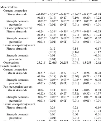
Table 7 displays the results of these regression models, where past and future oc-cupational trajectories are computed over eight-, ten-, and 12-year intervals.21The table demonstrates that both current and past occupational characteristics affect BMI in the expected manner for male workers, but that future occupational charac-teristics are unrelated. This is a significant result, since these regressions are designed to provide future characteristics with as much statistical power as past characteris-tics: Both are computed over the same length of interval, and both are residualized by regressing on current characteristics. Because the timing of occupation seems to matter, it is unlikely that fixed latent characteristics drive both occupation and weight, and it is similarly unlikely that weight variation drives future variation in
18. Clearly, a regression that did not use residualized versions of past and future occupational characteristics would produce the same fit as the one described above. However, it would not necessarily produce the same coefficients on the variables of interest, because current occupational characteristics would affect both the past and future occupational trajectories. Therefore, the overall effect of current occupation would be apportioned across all variables; this would make the test results much harder to interpret. Note that this test is more con-servative than it could be, because we leave information about the past inside future occupational data. 19. For example,
20. We regress past fitness demands on current fitness demands (and nothing else), past strength demands on current strength demands, and so forth.
Table 7
BMI and the Timing of Exposure to Physical Demands on the Job
Length of Past and Future Intervals
8 Years 10 Years 12 Years
Male workers Current occupation
Fitness demands – 0.40** – 0.39** – 0.48** – 0.46** – 0.53** – 0.48** (0.15) (0.17) (0.17) (0.19) (0.20) (0.22) Strength demands 0.02** 0.02** 0.03** 0.03** 0.03** 0.02**
percentile (0.01) (0.01) (0.01) (0.01) (0.01) (0.01) Past occupationjcurrent
Fitness demands – 0.24 – 0.34* – 0.36* – 0.47** – 0.41* – 0.53** (0.15) (0.18) (0.18) (0.21) (0.22) (0.24) Strength demands 0.02** 0.02** 0.02** 0.02** 0.03** 0.02**
percentile (0.01) (0.01) (0.01) (0.01) (0.01) (0.01) Future occupationjcurrent
Fitness demands – 0.12 – 0.14 – 0.17
(0.15) (0.16) (0.17)
Strength demands – 0.01 – 0.01 – 0.01
percentile (0.01) (0.01) (0.01)
Observations 25,215 22,665 20,255 17,761 15,253 12,827 Female workers
Current occupation
Fitness demands – 0.27* – 0.28 – 0.27 – 0.27 – 0.26 – 0.28 (0.16) (0.18) (0.18) (0.20) (0.21) (0.23) Strength demands 0.03** 0.03** 0.03** 0.03** 0.03** 0.04**
percentile (0.01) (0.01) (0.01) (0.01) (0.01) (0.01) Past occupationjcurrent
Fitness demands 0.04 0.21 0.00 0.14 – 0.06 0.03 (0.22) (0.28) (0.27) (0.32) (0.32) (0.37) Strength demands 0.02** 0.02** 0.03** 0.03** 0.03** 0.04**
percentile (0.01) (0.01) (0.01) (0.01) (0.01) (0.01) Future occupationjcurrent
Fitness demands 0.26 0.22 0.19
(0.20) (0.21) (0.23)
Strength demands 0.00 0.00 0.01
percentile (0.01) (0.01) (0.01)
Observations 23,236 20,658 18,491 15,997 13,962 11,552
*Significant at 10 percent; **significant at 5 percent.
occupational decisions. These are two important channels of selection, although by no means the only possible channels. None of our tests can rule out the existence of latent time-varying characteristics that cause occupational transitions and then
delayed changes in weight. Such a mechanism produces temporal orderings that
are observationally equivalent to a causal mechanism.
Future characteristics are not significant predictors for female workers either, but fitness demands—past or current—are also unrelated to BMI. This is consistent with the explanation that fitness demands are poorly measured for female workers. Past and current strength percentiles do seem to affect female BMI in the expected manner; there is no evidence that current weight influences future trajectories in strength demands. Therefore, it appears that selection for female workers occurs primarily at baseline, where heavier women sort into jobs requiring more strength.
V. Conclusion
We have presented evidence suggesting that occupation has a real effect in the determination of weight for male workers. This could be the direct re-sult either of more activity on the job, or of the fact that a more demanding job causes an individual to stay fitter. For female workers, on the other hand, there is no clear evidence of an effect, due in part to poor measurement of job character-istics for females, and due to baseline occupational selection of female workers by weight status. A male worker who spends 18 years in the most fitness-demanding occupation has a Body Mass Index 3.5 full units (24.7 pounds) lighter than a per-son in the least demanding occupation. Comparatively little of this relationship seems due to selective transition into and out of jobs by individuals of different weights.
The data are not conclusive enough to support an explanation of how and why males and females differ, but several possibilities emerge. First, causal effects could be smaller for females, because they expect less lifetime labor force attachment and engage in relatively more leisure-time or home production activities that have their own levels of exercise. Alternatively or additionally, selective pressures could be more severe for females, if a smaller proportion of women are able to perform stren-uous on-the-job activities. As such, that specific subgroup may be ‘‘funneled’’ toward strenuous jobs, while no such selection is necessary for male workers. It is also pos-sible that causal effects do exist for women, but that the DOT occupation data are not measured well enough for female workers to permit this inference.
would help us disentangle the relationship between on-the-job exercise and incen-tives for off-the-job exercise. A fuller picture of exercise and weight requires better data on exercise away from work.
Appendix 1
Occupation Data from the DOT
Our study links data on occupations from the Dictionary of Occupation Titles (DOT) to NLSY survey data. This appendix discusses the occupational data and how it is linked to the NLSY.
A. Linking Procedure
The 1991 DOT data are based on the DOTÕs own occupational taxonomy, which is distinct (and much more detailed) than the Census taxonomies typically found in the NLSY. To link these data to the NLSYÕs 1970 Census taxonomy, we use the National Occupational Information Coordinating Committee (NOICC) crosswalk be-tween the DOT occupation codes and the two Census classification systems.22The NOICC crosswalk assigns each DOT occupation code to exactly one 1970 Census code. However, because the DOT taxonomy is so much more detailed, each census code ends up associated with many DOT codes, and possibly many different values for occupational characteristics.
To solve this problem, we adopt the approach of England and Kilbourne (1989), who faced a similar problem in linking a Current Population Survey-based version of the 1977 DOT (which used 1970 census codes) to the 1980 census taxonomy of occupations. They computed mean characteristics within each 1980 census code. Similarly, we compute mean characteristics within each 1970 census code, by aver-aging over all the relevant DOT occupation codes linked to each 1970 code. We have found that various ways of weighting these averages—for example, by sex-specific proportion of the labor force in various years—produce nearly identical quantitative results. In the interests of simplicity and ease of interpretation, therefore, we con-struct unweighted averages, just as England and Kilbourne do.
B. Distribution of Physical Demands
The overall distribution of physical demands for male and female workers was dis-cussed in the text. As Figure A1 documents, this distribution changes for male work-ers very slightly with the aging of the NLSY cohort, with the most strenuous jobs becoming a bit less prevalent. However, Figure A2 shows that the distribution for fe-male workers does not even change by this much over time. These results suggest that changes over time in the effects of occupation are not likely to be driven by changes in occupational composition that accompany life-cycle transitions into less strenuous jobs.
Figure A1
Change Over Time in the Distribution of Physical Demands, Male NLSY Workers.
Source: NLSY, indicated years.
walla
and
Philipson
Figure A2
Change Over Time in the Distribution of Physical Demands, Female NLSY Workers.
Source: NLSY, indicated years.
The
Journal
of
Human
Appendix 2
NLSY Data
A. Height and Weight
The NLSY asked respondents to self-report their current height in the 1982 and 1985 survey years. We use the most recent height in all our analysis.
The NLSY asked respondents to self-report weight in the following survey years: 1981, 1982, 1985, 1986, 1988, 1989, 1990, 1992, 1993, 1994, 1996, 1998, 2000.
Height and weight are available in: 1982, 1985, 1986, 1988, 1989, 1990, 1992, 1993, 1994, 1996, 1998, and 2000. We report results from all these years.
B. Schooling
The NLSY asks: ‘‘What is the highest grade or year of regular school that you have completed and gotten credit for?’’ The answer to this question is coded as Grades 1– 12, and the number of years of post-high school education. Based on this variable, we define ‘‘high school dropouts’’ as having completed less than the 12th grade, ‘‘high school graduates’’ as having completed the 12th grade but no more, ‘‘college attend-ees’’ as having at least one but less than four years of post-high school education, and ‘‘college graduates’’ as having at least four years of post-high school education.
C. Earnings
For each individual, we compute her decile in the annual sex-specific earnings dis-tribution; this decile measure is used in our regressions. Since BMI is measured at the time of the interview, we measure earnings for thecurrentcalendar year, rather than the previous calendar year. For example, to construct 1986 earnings, we take the value from the 1987 survey, in which the respondent is asked to report his 1986 earn-ings. Moreover, since respondents are never explicitly asked about 1994, 1996, 1998, or 2000 earnings (only 1993, 1995, 1997, and 1999 earnings), we exponentially in-terpolate to obtain values for these years. The inin-terpolated values are defined only if the person reports nonzero earnings in both adjacent years. In the case of 2000, we extrapolate the growth observed from 1998 to 1999, and impute the variable only when both years are nonmissing and the individual reports working in 2000.
D. Occupation
We measure occupation as the respondentÕs primary (or CPS) occupation in the NLSY. Respondents are asked about their current or most recent job, and their an-swer is coded according to the 1970 Census occupational taxonomy.
Sensitivity analyses suggest that incomplete occupation histories do not substan-tially alter our results. Quantile and OLS regressions run on sex-specific pooled sam-ples of workers who reported at least 10 of 12 possible occupation-years were qualitatively similar to models run on the full sample.
References
Abe, T., K. Kojima, C. F. Kearns, H. Yohena, and J. Fukuda. 2003. ‘‘Whole Body Muscle Hypertrophy from Resistance Training: Distribution and Total Mass.’’British Journal of Sports Medicine37(6):543–45.
Appel, L. J., C. M. Champagne, D. W. Harsha, L. S. Cooper, E. Obarzanek, P. J. Elmer, V. J. Stevens, W. M. Vollmer, P. H. Lin, L. P. Svetkey, S. W. Stedman, and D. R. Young. 2003. ‘‘Effects of Comprehensive Lifestyle Modification on Blood Pressure Control: Main Results of the PREMIER Clinical Trial.’’Journal of the American Medical Association
289(16):2083–93.
Averett, Susan, and Sanders Korenman. 1996. ‘‘The Economic Reality of the Beauty Myth.’’ Journal of Human Resources31(2):304–30.
Barlevy, Gadi. 2001. ‘‘Why Are the Wages of Job Changers So Procyclical?’’Journal of Labor Economics19(4): 837–78.
Biddle, Jeff E., and Daniel S. Hamermesh. 1998. ‘‘Beauty, Productivity, and Discrimination: Lawyer’s Looks and Lucre.’’Journal of Labor Economics16(1):172–201.
Bound, John, C. Brown, and N. Mathiowetz. 1999. ‘‘Measurement Error in Survey Data.’’ InHandbook of Econometrics, ed. James Heckman, and Edward Leamer. New York: Springer-Verlag.
Case, Anne, and Angus Deaton. 2003. ‘‘Broken Down by Work and Sex: How Our Health Declines.’’ Working Paper 9821, National Bureau of Economic Research. Cambridge, Mass.: National Bureau of Economic Research.
Cawley, John. 2000. ‘‘Body Weight and Women’s Labor Market Outcomes.’’ Working Paper 7841, National Bureau of Economic Research. Cambridge, Mass.: National Bureau of Economic Research.
———. 2004. ‘‘The Impact of Obesity on Wages.’’Journal of Human Resources39(2): 451–74.
Chou, Shin-Yi, Michael Grossman, and Henry Saffer. 2004. ‘‘An Economic Analysis of Adult Obesity: Results from the Behavioral Risk Factor Surveillance System.’’ Journal of Health Economics23(3):565–87.
Costa, Dora, and Richard Steckel. 1995. ‘‘Long-Term Trends in Health, Welfare, and Economic Growth in the United States.’’ Historical Working Paper 76, National Bureau of Economic Research. Cambridge, Mass.: National Bureau of Economic Research. Cutler, David M., Edward L. Glaeser, and Jesse M. Shapiro. 2003. ‘‘Why Have Americans
Become More Obese?’’Journal of Economic Perspectives17(3):93–118.
Flegal, Katherine M., Margaret D. Carroll, R. J. Kuczmarski, and Clifford L. Johnson. 1998. ‘‘Overweight and Obesity in the United States: Prevalence and Trends, 1960–1994.’’ International Journal of Obesity and Related Metabolic Disorders22(1):39–47.
Flegal, Katherine M., Margaret D. Carroll, Cynthia L. Ogden, and Clifford L. Johnson. 2002. ‘‘Prevalence and Trends in Obesity among U.S. Adults, 1999–2000.’’Journal of the American Medical Association288(14):1723–27.
Gin, H., V. Rigalleau, and L. Baillet. 2003. ‘‘[Diet and Physical Activity in Type 2 Diabetes Prevention].’’Revue du Praticien53(10):1074–77.
Hill, James O., H. R. Wyatt, G. W. Reed, and J. C. Peters. 2003. ‘‘Obesity and the Environment: Where Do We Go from Here?’’Science299(5608):853–55.
Jovanovic, Boyan. 1978. ‘‘Job Matching and the Theory of Turnover.’’Journal of Political Economy87(5):972–90.
Katzmarzyk, P. T., and C. L. Craig. 2002. ‘‘Musculoskeletal Fitness and Risk of Mortality.’’ Medicine and Science in Sports and Exercise34(5):740–44.
Kell, R. T., G. Bell, and A. Quinney. 2001. ‘‘Musculoskeletal Fitness, Health Outcomes and Quality of Life.’’Sports Medicine31(12):863–73.
Knowler, W. C., E. Barrett-Connor, S. E. Fowler, R. F. Hamman, J. M. Lachin, E. A. Walker, and D. M. Nathan. 2002. ‘‘Reduction in the Incidence of Type 2 Diabetes with Lifestyle Intervention or Metformin.’’New England Journal of Medicine346(6):393–403. Lakdawalla, Darius N., and Tomas J. Philipson. 2002. ‘‘Technological Change and the Growth
of Obesity.’’ Working Paper 8946, National Bureau of Economic Research. Cambridge, Mass.: National Bureau of Economic Research.
Lakdawalla, Darius, Tomas Philipson, and Jay Bhattacharya. 2005. ‘‘Welfare-Enhancing Technological Change and the Growth of Obesity.’’American Economic Review: AEA Papers and Proceedings95(2):253–57.
Lee, Lung-fei, and Jungsywan H. Sepanski. 1995. ‘‘Estimation of Linear and Nonlinear Errors-in-Variables Models Using Validation Data.’’Journal of the American Statistical Association90(429):130–40.
Maiorana, A., G. O’Driscoll, L. Dembo, C. Goodman, R. Taylor, and D. Green. 2001. ‘‘Exercise training, vascular function, and functional capacity in middle-aged subjects.’’ Medicine and Science in Sports and Exercise33(12):2022–28.
Maiorana, A., G. O’Driscoll, C. Goodman, R. Taylor, and D. Green. 2002. ‘‘Combined Aerobic and Resistance Exercise Improves Glycemic Control and Fitness in Type 2 Diabetes.’’Diabetes Research and Clinical Practice56(2):115–23.
Mokdad, A. H., M. K. Serdula, W. H. Dietz, B. A. Bowman, J. S. Marks, and J. P. Koplan. 2000. ‘‘The Continuing Epidemic of Obesity in the United States.’’Journal of the American Medical Association284(13):1650–51.
———. 1999. ‘‘The Spread of the Obesity Epidemic in the United States, 1991–1998.’’ Journal of the American Medical Association282(16):1519–22.
Philipson, Tomas J., and Darius N. Lakdawalla. 2006. ‘‘The Economics of Obesity.’’ InElgar Companion to Health Economics, ed. Andrew M. Jones. Cambridge, U.K.: Edward Elgar.
Philipson, Tomas J., and Richard A. Posner. 1999. ‘‘The Long-Run Growth in Obesity as A Function of Technological Change.’’ Working Paper 7423, National Bureau of Economic Research. Cambridge, Mass.: National Bureau of Economic Research.
Putnam, Judith Jones. 2000. ‘‘Major Trends in U.S. Food Supply: 1909–99.’’Food Review 23(1):8–15.
Putnam, Judith Jones, and Jane E. Allshouse. 1999. ‘‘Food Consumption, Prices, and Expenditures, 1970–97.’’ Statistical Bulletin 965, Economic Research Service, U.S. Department of Agriculture. Washington, D.C.: Economic Research Service, U.S. Department of Agriculture.
Putnam, Judy, Jane Allshouse, and Linda Scott Kantor. 2002. ‘‘U.S. Per Capita Food Supply Trends: More Calories, Refined Carbohydrates, and Fats.’’Food Review25(3): 2–15.
Seidell, J. C., and I. Deerenberg. 1994. ‘‘Obesity in Europe: Prevalence and Consequences for Use of Medical Care.’’Pharmacoeconomics5(Suppl 1):38–44.