Thomas G. Koch is an economist with the Federal Trade Commission. Scholars who wish to attain the key variables used here may apply to CFACT Data Center. The author is willing to offer guidance. The appendix mentioned in this paper can be found at jhr.uwpress.org. This research was supported by the Non- Senate Faculty Fund at UC- SB. The research in this paper was conducted at the CFACT Data Center, and the support of AHRQ is acknowledged. The results and conclusions of this paper are those of the author and do not indicate concurrence by AHRQ or the Department of Health and Human Services. The views expressed in this article are those of the author and do not necessarily refl ect those of the Federal Trade Commission. The data used in this article can be obtained from the author beginning March 2016 through April 2019 from 600 Pennsylvania Avenue NW, M- 8059, Washington D.C. 20580. Telephone: 512- 809- 8014. Email: tkoch.at.ftc.gov.
[Submitted June 2013; accepted May 2014]
ISSN 0022- 166X E- ISSN 1548- 8004 © 2015 by the Board of Regents of the University of Wisconsin System
T H E J O U R N A L O F H U M A N R E S O U R C E S • 50 • 4
All Internal in the Family?
Measuring Spillovers from
Public Health Insurance
Thomas G. Koch
KochABSTRACT
Measurements of the impact of public health insurance have typically focused on the health and insurance outcomes of the newly eligible child. In this paper, I investigate the consequences of public health insurance for the other members of the household. Using a regression discontinuity design, I fi nd that a child’s public health insurance eligibility crowds out the private health insurance of parents by 11 percentage points when it is not accompanied by parental eligibility. This loss of insurance corresponds to changes in self- reported health and preventive care for women.
I. Introduction
Measurements of the impact of public health insurance have focused on the outcomes of the newly eligible child. Starting with Cutler and Gruber (1996) and Currie and Gruber (1996a), the consequences of Medicaid on insurance and uti-lization were child- centric—measuring the crowdout of children’s private insurance or whether the number of children’s lives saved by public health insurance satisfi ed cost- benefi t analysis. Pregnant women were also considered, but, with few exceptions, economists have measured the impact of own eligibility on own outcomes.
medical insurance in the employer- provided market is explicitly oriented around fam-ily structure. Public insurance was being given to individuals (children) who were expressly part of a larger unit (the family) that shares a budget constraint.
Using detailed family- level data and state- year- age public insurance eligibility guidelines, I estimate the causal impact of children’s public health insurance eligibil-ity on the insurance received by the adults within the child’s household, as well as on the quantity and quality of the parents’ healthcare. These effects are estimated using a regression discontinuity design based upon the income thresholds used to determine child eligibility. Making a child eligible for public health insurance without making the adult also eligible decreases the incidence of health insurance among the adults in the same household by 11 percentage points. This is due to a large and statistically signifi cant decrease in the incidence of private health insurance among those adults. This decrease in private health insurance is associated with decreases in the use of some preventive care and with lower self- reported health.
Previous investigations on the causal effects within a child’s household have been limited to searching for potential instruments, as in Gruber and Simon (2008). Yet little, if anything, is known about the external impact on the family of a newly eligible child. Cutler and Gruber (1996) estimated the impact of Medicaid expansions for chil-dren and pregnant women for the private health insurance on adults. Their focus on adult men who were not the subject of those earlier expansions points to spillovers, though their focus is limited to insurance outcomes. Monheit and Vistnes (2010) used the variation in the parent versus child insurance patterns (private and private versus private and public, for example) but cannot rule out that the insurance patterns are endogenous.
My fi ndings also add texture to the “job lock” literature that, starting with Madrian (1994), found that workers were hesitant to switch jobs due to health insurance. More to the point of this paper, Garthwaite, Gross, and Notowidigdo (2014) found that an expansion of public health insurance in Tennessee decreased labor supply (on the extensive margin) likely because it relieved such pressures.
My fi ndings are also distinct from the measurements of parental eligibility on pa-rental outcomes. Busch and Duchovny (2005), Hamersma and Kim (2009, 2013), and Aizer and Grogger (2003) perform the classical crowdout analysis in this fashion. Here, I am able to isolate the effects of child eligibility on parental outcomes, which refl ects a spillover rather than a direct effect. The estimates presented here complement the fi ndings of Koch (2013), which used the same identifi cation strategy to measure the causal impact of eligibility on the newly eligible child. My analysis expands our understanding of how these policies impact the broader population. Like Leininger, Levy, and Schanzenbach (2010), which measured the effect of eligibility on household consumption, focusing on the household provides a broader picture of how public insurance impacts families. The impact on spending measures the consumption- based welfare effects. By measuring the external (aside from the child, within the house-hold) consequences of eligibility, my estimates capture a more complete picture of the impact on healthcare utilization of Medicaid and State Children’s Health Insurance Program (SCHIP).
health-Koch 961
care and health are in fact the very same. The design of the Oregon lottery measures the treatment effect for the average of the lottery- eligible adults. In contrast, this study focuses on the local treatment effect for the parents of the marginally eligible child. This study considers these marginal parents in all sampled states, so it may be con-sidered more general in some ways, as Koch (2013) fi nds a great deal of variation in treatment effects across states.
My work also relates to Anderson, Dobkin, and Gross (2012), which uses regression discontinuity on a different threshold—the age 19 cutoff for public health insurance plans. Similarly, they estimated a large drop from public to no insurance, though they had limited data on medical spending and its sources. Their fi ndings on emergency and inpatient care are not a contradiction to my work; they focus on a separate population, using a different source of identifi cation. Moreover, their estimated dropoff in insur-ance is ostensibly forced as children age out of insurinsur-ance, while the rise in uninsurinsur-ance here is at least partly a matter of choice.
A similar RD design was employed in two studies of the causal effects of Medi-care—Card, Dobkin, and Maestas (2009) and Card, Dobkin, and Maestas (2008). Like Anderson, Dobkin, and Gross (2012), a discontinuity in age, not income, was used to fi nd the causal impact of a separate public insurance program. Those studies focused on the impact of Medicare as it creates near- universal insurance for the newly elderly population. The predominant transition under study here, the switch from private to no insurance, is related to studying the universalization of insurance due to Medicare. This is, again, a test of the generalizability of the results for Medicare to the broader adult population.
Use of age cutoffs raises a more general concern that the strategy used here avoids. When using an RD design in age, the empirical specifi cation compares the just- eligible to the about- to- be- eligible. Absent extreme discounting, the treatment effect calculated with that comparison may not be valid when individuals gain or lose eligibility with something less than exact predictability.
Previous estimates, such as those found in Currie and Gruber (1996a, 1996b), found that increasing the number of eligible children would lead to increases in the quality and quantity of care. While seminal contributions to the literature, their data were limited either to survey questions of healthcare use (“Did you go to the doctor in the previous year?”) or focused measures of utilization on special groups (the healthcare quantity and outcomes of pregnant women and their newborn children). Here, we can bridge those two works by utilizing data that is both focused on a variety of healthcare outcomes but also provides a representative sample of those on the margin of public policy.
II. A Theory of Crowdout and Group Insurance
Consider a household H with N = size(H) members. In the absence of public programs, full insurance has value πi to each member i∈H. The cost of insuring each member is pi. In a market unfettered by household- level constraints, a member of the household is insured if πi > pi and not otherwise.
the child. Thus, it may be the case that the parent would not take up employer- provided insurance him- or herself (πparent < pparent) but would when that insurance is bundled with insurance for a dependent (πparent + πdependent > pparent + pdependent).
Also, with group insurance, there is a disconnect between individual- level charac-teristics, such as health and expected medical costs, and the price of insurance. In a competitive market with symmetric information, we would expect πparent + πdependent > pparent + pdependent to hold as a consequence of each component inequality πi > pi via risk aversion. However, with group insurance, each component inequality may not hold. When a child becomes eligible for public health insurance, this provides a low- cost and lower- quality substitute for private insurance.1 The theoretical model of Cutler and Gruber (1996), itself an extension of Peltzman (1973), describes why and when this would happen. The public insurance offer will diminish the consumer surplus from private health insurance, πdependent – pdependent, and potentially reverse the household- level insurance bundle choice.
The effects measured here may not be due purely to changes in insurance. The switching of children from private to public insurance, and the dropping of insurance for the parent altogether, coincides with a pretax growth in income, pparent + pdependent, or whatever fraction of that is returned to the employee when insurance is not part of compensation. If healthcare (both quantity and quality) is more normal than other goods, this should bias the estimates up (that is, make them less negative).
III. Data and RD Design
In order to estimate the impact of public health insurance eligibility on health insurance and healthcare outcomes, we need a data set that combines mea-surements of household labor supply and income to determine eligibility, as well as healthcare utilization and spending. The Medical Expenditure Panel Survey (MEPS) is ideally suited to the task. The MEPS is a short- panel data set starting in 1996 that covers nationally representative samples of the United States. It includes measures of an individual’s health, healthcare utilization, insurance status, and related information, such as labor market outcomes and family structure. Five interviews are conducted over two years for each panel, and information about the entire household is collected. Monthly insurance variables and annual utilization and expenditure data are among the publicly available data.
Individual- level data, such as age, gender, employment status, and health insurance coverage and its sources, are collected for each member of the household. Because a child’s eligibility may well depend upon his or her age, this level of detail is essential. For each individual job reported, there is a reported wage and hours worked. Because a child’s eligibility depends upon the household’s income, information on all jobs held by members of the household is required.
Whether a child is eligible for public health insurance depends upon an income test—is the household income larger or smaller than some multiple of the house-hold’s Federal poverty guideline? The househouse-hold’s Federal poverty guideline depends
Koch 963
upon household structure, which is available in the public data. However, which mul-tiple depends upon the state of residence and age of the child. State of residence is not publicly available in the MEPS due to confi dentiality concerns. Measurements of eligibility were constructed by the Agency for Healthcare Research and Quality (AHRQ), which administers the MEPS; these variables for 1996 to 2005 were made available to this researcher under a confi dentiality agreement. The eligibility variables were not constructed for their parents. The eligibility thresholds were calculated by AHRQ but were not made available to this researcher. The thresholds are required to determine the distance of the household from eligibility, which is key for the empirical investigation below. In lieu of AHRQ’s measures of eligibility, the MEPS data have been merged with eligibility rules from the TRIM3 database, which is a collection of welfare rules constructed by the Urban Institute and van Kerm (1999), which provides the relevant guidelines by year and family structure. (The actual merging by state, year, and age was performed by an AHRQ contractor to satisfy the confi dentiality requirements.) This information was supplemented by the eligibility rules published in a series of reports by the Kaiser Family Foundation (Cohen Ross and Cox 2000, 2002). These rules include the state- year- age specifi c eligibility thresholds for SCHIP, Medicaid and Medicaid extension programs, as well as the rules governing income disregards. Income and eligibility may well be measured with error, and the online appendix contains robustness exercises to evaluate the likelihood and consequences of this possibility.2
The SCHIP expansion began in 1997 and provided funds for states to expand the number of children eligible for public health insurance. As documented in Figure 1, once fully implemented in the early 2000s, SCHIP doubled the number of children eligible for public health insurance. Its consequences for the number of children who actually had insurance were not as impressive. As seen in Figure 2, this large expan-sion of public health insurance coincided with similarly sized decreases in the number of children privately insured.
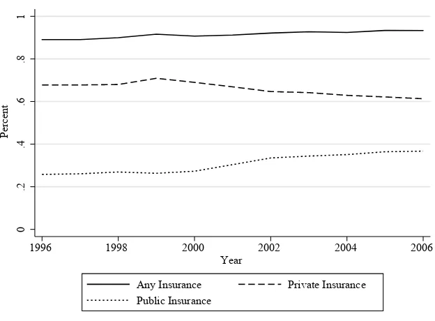
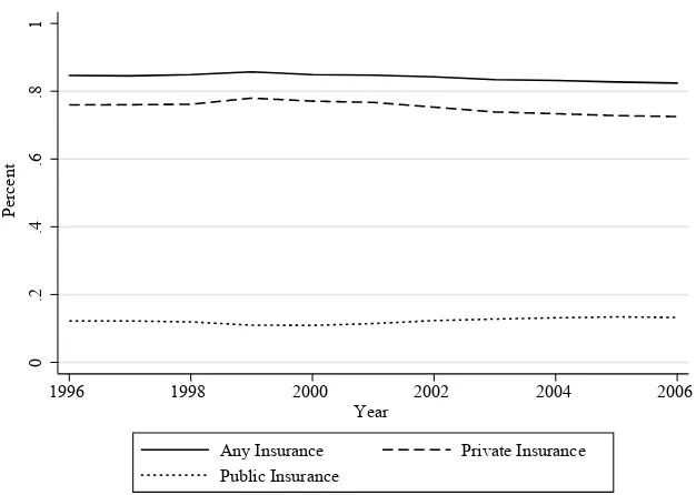
The growth in children’s public health insurance did not have a corresponding change in the nonelderly adult population. Figure 3 plots the incidence of public health insurance for nonelderly adults over this time period along with the rates of private and any insurance. This fi gure does not demonstrate a consistent decrease in the incidence of private health insurance or any health insurance at all over this period. However, as Figure 2 is not proof of crowdout among children, this fi gure does not demonstrate that parental insurance did not respond to the public insurance options of children. The nature of eligibility rules allows for a regression discontinuity (RD) design estimation. SCHIP expansions were either literal expansions of Medicaid or new programs whose eligibility rules were similarly constructed. In either case, eligibility for public insur-ance depends upon the ratio of family income to the Federal poverty guideline. A key
0
.2
.4
.6
.8
1
P
erc
ent
1996 1998 2000 2002 2004 2006
Year
Any Eligibility SCHIP
Medicaid
Figure 1
Public insurance eligibility for children.
Figure 2
Insurance rates for children.
0
.2
.4
.6
.8
1
P
erc
ent
1996 1998 2000 2002 2004 2006
Year
Koch 965
eligibility criterion is met if this ratio is smaller than a threshold, which depends upon the age of the child, state of residence, and year. The implementation of SCHIP plans lead to dramatic increases in the eligibility thresholds across states.
A. Design Implementations
Does public insurance alter the incidence of insurance and the incidence and treatment of disease? Suppose I attempt to measure the effect of public medical insurance on healthcare demand using the equation below:
(1) ci = Liγc + Xiβc + εc,i
where ci is adult i’s insurance or healthcare outcome under study; Liis equal to one if the child in adult i’s household is eligible for public insurance; Xi is a set of other relevant information, such as race, ethnicity, age, and state of residence;3 and ε
c,i is the
usual residual. What does γc measure? First, since this is a measurement of eligibility and not of takeup, there is no takeup endogeneity bias. In part, γc measures the causal effect of public insurance eligibility on the healthcare outcome. However, because eligibility is determined by family income and the child’s age, it also picks up the outstanding correlation between income and demand for healthcare. For example, if health is a normal good, without controls for income, γc would be biased down.
3. The AHRQ made available a coded variable that allows observations to be grouped by state but does not disclose the identity of the states.
0
.2
.4
.6
.8
1
P
erc
ent
1996 1998 2000 2002 2004 2006
Year
Any Insurance Private Insurance
Public Insurance
Figure 3
In order to overcome this, I employ a regression discontinuity design, similar to Card and Shore- Sheppard (2004) in their study of Medicaid expansion. Now, the fol-lowing equation is estimated:
(2) ci = Liγc+ Xiβc + G(distancei, Family Incomei) + εc,i,
where G(distancei, Family Incomei) is a nonlinear function of family income and “distance” from the eligibility threshold (that is, family income as a fraction of the poverty guideline less the governing threshold). This distance measure is the forcing, or running variable, as it determines eligibility. The effects picked up by G need not be causal—it just needs to pick up all of the covariation between the outcome variable and the variables that determine eligibility, beyond the causal effects of eligibility itself. Adding these controls leaves γc to measure the effect of public insurance itself. Concerns about the many eligibility thresholds exploited here are addressed when γc
is estimated by eligibility thresholds.
For the preferred specifi cations, G(distancei, Family Incomei) is linear in distance from the eligibility guideline and the family income as a fraction of the poverty guide-line. This last term is added because the relevant guidelines vary dramatically over the period of study.4 Family income includes all nonself- employed wage income within the CPS- type family, and poverty guidelines are calculated accordingly. The public insurance variable, Li, is equal to one if eligible for Medicaid or SCHIP, zero other-wise. Because the MEPS is collected using a complex survey design, all estimates and standard errors are calculated using appropriate weights, strata, and PSU. Because the measures that determine eligibility are close to continuous (income is measured in dol-lars and cents), there is no need to cluster according to a discrete forcing variable, as in Lee and Card (2008). Similarly, the variation being exploited here is in the income distribution in the cross- section and not across time and state (as would be the case for simulated eligibility); thus, there is not the usual reason to cluster by the determinants of eligibility threshold: state and year. The estimates provided below are pooled across the short (twice- observed) panel. Given the panel nature of the data, clustering by individual may be appropriate. In the online appendix, I demonstrate that using only the fi rst of two observations per individual has the expected and modest impact on statistical inference.
Because family income- to- poverty guideline ratios vary greatly within the popula-tion, Equation 2 is estimated using a restricted subsample, where the household has to be within one and a half Federal poverty guidelines from the child’s eligibility threshold. The main specifi cation of Equation 2 requires only a control function G. However, I can also add other control variables, such as a polynomial in adult age in months, and dummy variables for race, Hispanic ethnicity, and whether the parent is a single mother. Year- and state- fi xed effects are also included. The sample and subsample means are reported in Table 1. The subsample represents a group of adults well distributed over age groups. (The age groups presented were constructed to be of similar size.) The subsample is 78 percent white and 16 percent black.
Most of the specifi cations below employ a linear- probability model, save for the few spending and utilization outcomes considered. Because some of the specifi cations
K
oc
h
967
Table 1
Means of the sample
Mean Mean
Variable Full Sample Subsample Variable Full Sample Subsample Subsample N
Demographics Spending and Self- Reported Health
Age: 18 years- 0.1844 0.2187 Total 1,967.13 1,898.30 37,121
27 years, 1 month- 0.1949 0.231 Offi ce- based 442.77 408.54 37,121
33 years, 11 months- 0.2068 0.205 Out- of- pocket 360.76 320.74 37,121
39 years, 6 months- 0.2206 0.1846
46 years, 1 month- 0.1934 0.1607 Excellent or very good 0.624 0.597 37,121
1 = Male 0.465 0.450
1 = White 0.800 0.774 Preventive Care—All
1 = Black 0.136 0.164 Flu shot 0.172 0.155 25,784
1 = Hispanic 0.165 0.221 BP check 0.762 0.736 25,478
Cholesterol check 0.432 0.386 24,664
Insurance by Source Annual exam 0.527 0.492 25,528
Private 0.684 0.642
Any 0.786 0.763 Preventive Care—Women
Public 0.125 0.148 Pap smear 0.640 0.618 14,256
Breast exam 0.643 0.617 14,264
N = 79,253 37,121 Mammogram 0.361 0.315 9,293
involve a robust set of state- and year- fi xed effects, OLS is preferred; those fi xed ef-fects are useful in distinguishing whether or not the mean shifts at the discontinuity.
For censored outcomes, the use of traditional estimators with a global polynomial has been advised by Imbens and Wooldridge (2009). The tables report a fi rst- order approximation of the marginal effects of the Tobit equation—⌽(Xi), the latent equa-tion estimate times the average fi tted probability that the observation is not censored. Due to the nonlinear nature of these estimates, the t- statistics for the underlying pa-rameter estimates are reported for consistency, as they are for the linear probability models.
I also provide graphical evidence of the discontinuities. In general, graphical anal-ysis can be carried out with the average value in “bins” according to the forcing vari-able, as advised by Imbens and Lemieux (2008). Here, the forcing variable is the difference (or distance in the graphs) between the ratio of family income to Federal poverty guideline and the relevant cutoff. The bins used here are as wide as 1 percent of the Federal poverty guideline. This corresponds to a $156- wide 1 percent bin for a family of four in 1996. A fl exible fi tting of the bin averages is also provided in the form of a local linear smoother. The weighting function of the local linear smoother uses a rectangular kernel, as advised by Lee and Lemieux (2010). The bandwidth of kernel is based upon the rule of thumb provided by Fan and Gijbels (1996, Sec-tion 4.2).5
B. Validity of the Design
In order to be valid, the regression discontinuity design needs to be robust to several key concerns. First, the forcing variable here, the fraction of family income to Federal poverty guideline, is a choice variable for the household. In many RD design settings, the forcing variable, such as date of birth, is not a matter of individual choice. That is suffi cient to satisfy concerns of “ducking” under the threshold. If you can exactly change your forcing variable to place yourself precisely below the threshold, then receiving the treatment is partially a matter of self- selection and is not as good as randomly assigned.
However, just because the forcing variable is infl uenced by the choices of the in-dividuals does not mean that an RD design is invalid. Conceptually, this is related to a key adverb used above: Can the forcing variable be manipulated to move precisely below the eligibility threshold? As discussed in Lee and Lemieux (2010), coarse ma-nipulation does not invalidate a RD design. In this context, individuals can vary their wage earnings by varying their hours or insurance choices in order to manipulate the numerator of the forcing variable. Alternatively, they could change their family struc-ture (that is, have a new child), which would increase the family’s Federal poverty guideline and increase the denominator.
The practical obstacles to precise manipulation should be clear. First, the household must know the administrative rules: the eligibility thresholds and the Federal poverty guideline, both of which change over time. Second, the ability of a worker to precisely change his or her wages may be limited. If a worker changes insurance options in
Koch 969
order to become eligible for public health insurance, the premiums are often large and predetermined subject to nondiscrimination policies. Similarly, it may be diffi cult for an employee to add or drop work hours exactly the precise number of hours needed to get just below the threshold. Finally, manipulating household structure may be costly, typically takes at least nine months, and adjusts the denominator of the forcing vari-able in a lumpy, discrete manner.
Moffi tt and Wolfe (1992) found that Medicaid generosity is negatively associated with labor supply. They measure labor supply as having a job, a rather coarse tool to achieve the kind of income- manipulation required to invalidate the RD design. Yelow-itz (1995) and Ham and Shore- Sheppard (2005) both study the effects of the eligibility thresholds themselves on labor supply (that is, working or not). Yelowitz (1995) fi nds a relationship under more restrictive econometric assumptions, while Ham and Shore- Sheppard (2005) fi nds that relaxing those restrictions diminishes the link between eli-gibility rules and labor supply. Similarly, Garthwaite, Gross, and Notowidigdo (2014) found evidence that public health insurance can be linked to decreases of labor supply on the extensive margin, in one particular recent example.
Hamersma (2013) studies the intensive margin (that is, hours) and wage growth. The author fi nds no evidence of “bunching” just below the eligibility threshold. The author does fi nd some evidence of a broader, less- exact relationship between wages and eligibility thresholds. Again, while this broad relationship between the eligibility rules and outcomes is of interest, the lack of a narrow and exact relationship supports the RD design requirement.
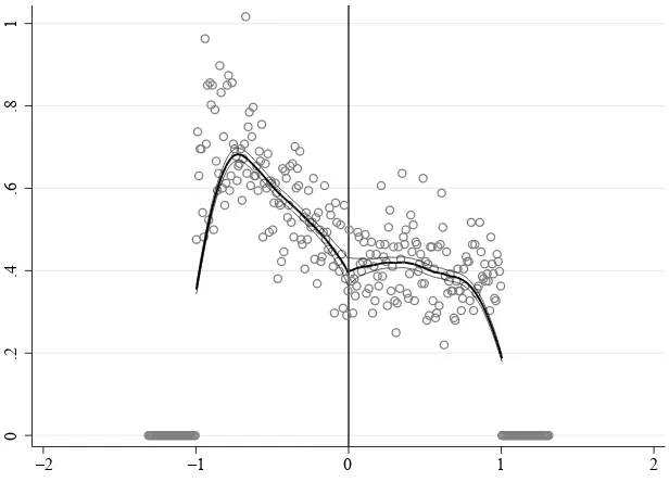
Validating a RD design with a forcing variable that can be manipulated need not be left to the imagination. McCrary (2008) suggests plotting the number of observations in each bin to test for this kind of manipulation. Such a graph in Figure 4 suggests a lack of precise manipulation. The estimated log- difference in density fi nds a 1 percent difference in smoothed density at the discontinuity with a standard error of fi ve times that value. Thus, the estimated change in density lacks both statistical and economic signifi cance. 6
The weekly wages and hours of the parents near the eligibility thresholds reinforce this result. Using the regression framework, neither demonstrates evidence that house-holds are manipulating their earnings or hours near the threshold. If they did, then we would expect an unusually small number of hours worked by households near the eligibility threshold. Likewise, households that manipulate their weekly wage to become just- eligible would have unusually low weekly earnings near the threshold. The regression estimates (not reported) are not statistically signifi cant, with t- statistics below one.
In the online appendix, I present evidence of manipulation using predetermined characteristics, using methods similar to Fang, Keane, and Silverman (2008). If there is no manipulation of the forcing variable, then the frequency of predetermined char-acteristics around the threshold should be constant. The graphs suggest a modest decrease in percentage black near the eligibility threshold. The estimates below are largely stable to the inclusion of demographic controls, including race.
IV. Results
Table 2 presents the estimated equations for insurance outcomes—the adult having private insurance, public insurance or any insurance at the time of the child’s eligibility determination. Estimates are reported for two specifi cations: fi rst, when the only repressors are linear controls for the forcing variable; and second, when state of residence, year, age, race, and single mother status are also included. The table also reports the estimates separately by gender of the parent and whether or not the parent shares an eligibility threshold with the child. That is, in addition to considering only parents whose child’s threshold is 1.85 times the poverty guideline, parents are excluded if they lived in those states for the years where adult extension programs existed per the TRIM3 or Kaiser Family Foundation sources listed above.7
As suggested by the theoretical model above, some adults do drop private health insurance with the eligibility of a child in the same household. In all, there is an 18 (if no additional controls are added) or 16 (if they are) percentage point decrease among parents who have private insurance. In the subsample, 64 percent of the parents have private health insurance, so this corresponds to a 25 percent change. The table also reports a three percentage point increase in takeup of public insurance at their child’s eligibility threshold. Parents may share eligibility thresholds with their children. The
7. Those states are Arizona, Wisconsin, Minnesota, and Massachusetts, for various years over the same. Other states, such as Iowa, offered extension programs at levels below the child eligibility thresholds.
0
.2
.4
.6
.8
1
–2 –1 0 1 2
Figure 4
K
oc
h
971
Table 2
Estimated effect with coeffi cient and t- statistics for child’s public insurance eligibility on same- household adults insurance
All Men Women Different Threshold
Private insurance –0.180*** –0.158*** –0.201*** –0.164*** –0.162*** –0.153*** –0.132*** –0.109***
(–11.09) (–10.39) (–9.75) (–8.13) (–9.28) (–9.44) (–6.60) (–5.61)
Any insurance –0.152*** –0.135*** –0.195*** –0.154*** –0.116*** –0.118*** –0.134*** –0.114***
(–9.82) (–9.05) (–9.37) (–7.55) (–6.99) (–7.19) (–7.77) (–6.79)
Public insurance 0.039*** 0.036*** 0.003 0.015 0.068*** 0.056*** 0.004 0.003
(3.52) (3.52) (0.22) (1.33) (4.66) (4.15) (0.38) (0.25)
N = 37,119 20,936 16.183 22,816
Demographic controls X X X X
Notes: Insurance outcomes are estimated using a linear probability model. All specifi cations include linear controls for family income- to- poverty guideline ratio and distance to eligibility threshold (denominated in the same). The fi rst column reports the coeffi cients and t- statistics when no other controls are included. The second column reports the same when year- and state- fi xed effects, as well as the demographic controls described in the text, are included. To be included in the estimation sample, the household of the adult must be within 1.5 Federal Poverty Guidelines of the relevant eligibility threshold.
net effect on overall insurance coverage is a 15 or 14 percentage point drop in having any insurance, or roughly 20 percent of the subsample’s overall coverage rate, inde-pendent of source. The online appendix describes in detail how these point estimates change when G is approximated using a higher order polynomial. In short, the magni-tudes vary modestly but the qualitative patterns remain.
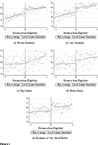
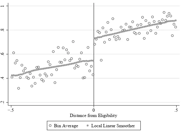
These estimates are supported by comparison to the local- linear estimates in Fig-ures 5a and 5b. The jump in the local linear smoother corresponds to the estimates in Table 2, allowing for a different style of fl exibility. These effects are smaller than the effects on children’s private health insurance found in Koch (2013). For reference, Figure 6 reproduces the graphical illustration of children’s eligibility on children hav-ing private health insurance. Likewise, the increase in public health insurance for adults is also one- half to one- third of that for children, suggesting that only a fraction of the adults share an eligibility threshold with their children.
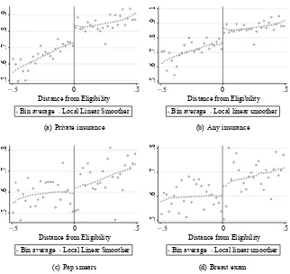
The plots of the data for the not- eligible parents, as well as the local linear regres-sions, can be found in Figures 7a to 7d for the outcomes of private insurance and any insurance. The bins of these fi gures are two percentage points of the Federal poverty guideline wide because the samples are smaller. They are still noisier than their coun-terparts for the entire sample. However, the local linear fi ts correspond to the point estimates presented in Table 3—a decrease in private and any insurance on the order of ten percentage points with an average incidence around the discontinuity of 73 per-cent, averaged across both genders. The insurance estimates are statistically signifi cant with confi dence intervals at 99 percent. These magnitudes are slightly smaller than the overall estimates. I have isolated the changes in adult insurance due to the changes in child public insurance options, so these estimates correspond to the spillover effects from child eligibility.
These results cannot be directly compared to the only other similar fi ndings in the literature. Cutler and Gruber (1996) used the percentage of family’s household average medical spending covered by public insurance, instead of whether a child was in-sured, to measure the impact of public coverage on household private coverage. When presenting the total amount of crowdout due to the Medicaid expansions between 1987 and 1992, they report that 600,000 children lost private coverage while half that number of men and women over the age of 44 (who would not have been eligible in those expansions) lost their private coverage. The private insurance estimates I fi nd are larger than the two- to- one ratio of child- to- adult loss of private coverage measured in Cutler and Gruber (1996), though it is exactly the two- to- one ratio when using the same third- order polynomial specifi cation as Koch (2013). That specifi cation uses a higher- order approximation for G and can be found in the online appendix.
Koch 973
In 1996, and starting again in 2000, the MEPS asked a series of questions about the most recent preventive care received by adults. In particular, all respondents were asked when their most recent checkup took place, as well as whether they received a fl u shot, a blood- pressure check, or a cholesterol check. Women were asked when they last had a pap smear, breast exam, and mammogram.
There is some limited evidence that a child’s eligibility impacts a mother’s chances of having more intensive annual preventive care. In the regression specifi cations, there is an eight to nine percentage point decrease in breast exams for women as a child be-comes eligible for public health insurance, with mixed results on the incidence of pap smears. These effects are similar to the local- linear estimates in Figure 5d for breast exams, though the graphical evidence in Figure 5c does not suggest an effect. The fi fth- order polynomial representation of G(·) further raises doubts about the robustness of the effects on pap smears.
There is no effect on mammograms (asked of women 30 years and older). This is likely because mammograms are much less frequent than the other two screen-ing exams. Regular mammogram screenscreen-ing is not recommended until a woman is in her 40s or 50s. For many younger women, the changes in insurance due to a child’s eligibility for public health insurance would not bind on her decision to (not) have a mammogram.
Table 3 also reports point estimates for the effects on blood pressure checks and an-nual exams that are statistically signifi cant. However, as noted in the online appendix,
.2
.4
.6
.8
1
í 0
Distance from Eligibility
Bin Average Local Linear Smoother
Figure 6
Koch 975
these estimates are particularly sensitive to the specifi cation of G, and the graphs for them (not reported) raise similar doubts.
There are instances where we might expect no effects. These cases can be useful tests for false- positives—is the RD design fi nding effects where there should be none? Flu shots are the least frequent form of preventive care and are often made available through employers or public health agencies. Table 3 fi nds there is no change in a par-ent having a fl u shot as his or her child becomes eligible for public health insurance.
Finally, the MEPS asks for an individual’s self- reported health status with fi ve po-tential answers; I aggregate them into two: Excellent and Very Good for “high health” answer and Good, Fair, or Poor for “low health.”8 There is an eight percentage point decrease in a parent’s self- reported health being in the highest two categories when a child in the parent’s household becomes eligible for public health insurance. This
cor-8. The results are similar if the “Good” responses are included in the “high health” group.
.5
T
he
J
ourna
l of H
um
an Re
sourc
es
The effects (and t- statistics) of a child’s public health insurance eligibility on adult outcomes
All Men Women Different Threshold
Spending, by source or use
Total –432.55** –294.40* –755.88** –300.26 –212.67 –199.75 –610.88** –400.90* (–2.53) (–1.94) (–2.39) (–1.24) (–1.59) (–1.47) (–2.48) (–1.85) Offi ce–based –87.69*** –64.28** –85.88** –37.46 –88.51** –80.82** –108.00*** –67.64**
(–3.31) (–2.31) (–2.58) (–1.07) (–2.52) (–2.28) (–3.37) (–2.07) Out- of- pocket –63.84*** –41.16* –83.53** –40.43 –48.13* –34.78 –63.22** –35.88
(–2.97) (–1.92) (–2.56) (–1.33) (–1.89) (–1.45) (–2.15) (–1.15)
Preventive care, All
Flu shot –0.013 –0.011 –0.014 –0.008 –0.013 –0.014 –0.023 –0.017
(–0.85) (–0.70) (–0.78) (–0.43) (–0.63) (–0.73) (–1.36) (–1.02) Blood pressure check –0.052*** –0.047*** –0.052** –0.033 –0.052*** –0.053*** –0.056*** –0.049**
(–3.12) (–2.97) (–2.25) (–1.46) (–2.95) (–3.07) (–3.21) (–2.85) Cholesterol check –0.046** –0.043** –0.054** –0.031 –0.040* –0.051** –0.028 –0.024 (–2.51) (–2.51) (–2.16) (–1.28) (–1.72) (–2.38) (–1.33) (–1.20) Annual exam –0.052*** –0.061*** –0.040 –0.032 –0.062*** –0.080*** –0.047** –0.051***
(–2.87) (–3.42) (–1.60) (–1.27) (–2.63) (–3.50) (–2.41) (–2.64)
Preventive care, Women
Pap smear –0.066*** –0.077*** –0.066*** –0.077*** –0.072*** –0.087***
(–2.98) (–3.65) (–2.98) (–3.65) (–2.96) (–3.66)
Breast exam –0.078*** –0.092*** –0.078*** –0.092*** –0.082*** –0.093***
(–3.46) (–4.34) (–3.46) (–4.34) (–3.26) (–3.79)
Mammogram –0.050* –0.057** –0.050* –0.057* –0.021 –0.028
(–1.82) (–2.18) (–1.82) (–2.18) (–0.72) (–0.98)
Self- reported health
Excellent or very good –0.076*** –0.078*** –0.057*** –0.067*** –0.090*** –0.090*** –0.059*** –0.053*** (–5.37) (–5.47) (–2.82) (–3.37) (–5.21) (–5.03) (–3.18) (–2.94)
Koch 977
responds to a 10–13 percent decrease in the reporting of excellent or very good health. Women’s reports of their own health are more responsive than that of men, and both are statistically signifi cant. In all instances, the magnitude of this effect is similar to the point estimates found in Finkelstein et al. (2012), which randomizes public health insurance in Oregon with a lottery.
Figure 5e supports the point estimates presented in Table 3. Because the changes in insurance and utilization are occurring at the same time, I cannot disentangle which, if either, is responsible for this change in self- reported health. The recent fi ndings of Finkelstein et al. (2012) suggest that much of this may be psychological, but the timeframe under study here is too broad to make a similar judgment.
V. Conclusion
Public health insurance for children has been shown to have conse-quences for children. But the prior literature has not examined its conseconse-quences for the child’s family. Using a regression discontinuity design in eligibility, this paper investigates how giving a child public health insurance can impact the members of that child’s household. In particular, there is a spillover of about eight percentage points where adults lose private health insurance when their child becomes eligible. There also are negative and statistically signifi cant decreases in preventive care associated with this loss of insurance.
This research reminds us that the consequences of public policy are beyond the scope of its target. While this idea is nothing new, it should not be surprising in this case. When states and the federal government expanded public health insurance in the late 1990s and early 2000s, children were the primary focus. As the theoretical model developed above suggests, it is unreasonable to expect this policy not to impact parents whose private health insurance decisions are directly linked to those for their children. Here, I have measured the quantitative impact of these policies upon the tangled nature of household insurance choices. This suggests that family- based public policy interventions can offset the potential adverse coverage and health consequences of child- centric policies for current- day adults.
References
Aizer, Anna, and Jeffrey Grogger. 2003. “Parental Medicaid Expansions and Health Insurance Coverage.” NBER Working Paper 9907.
Anderson, Michael, Carlos Dobkin, and Tal Gross. 2012. “The Effect of Health Insurance
Coverage on the Use of Medical Services.” American Economic Journal: Economic Policy
4(1):1–27.
Busch, Susan H., and Noelia Duchovny. 2005. “Family Coverage Expansions: Impact on
Insurance Coverage and Health Care Utilization of Parents.” Journal of Health Economics
24(5):876–90.
Card, David, and Lara D. Shore- Sheppard. 2004. “Using Discontinuous Eligibility Rules to
Identify the Effects of the Federal Medicaid Expansions on Low- Income Children.” Review
of Economics and Statistics 86(3):752–66.
Insurance Coverage on Health Care Utilization: Evidence from Medicare.” American Economic Review 98(5):2242–58.
———. 2009. “Does Medicare Save Lives?” Quarterly Journal of Economics 124(2):597–636.
Cohen Ross, Donna, Laura Cox, and Kaiser Commission on Medicaid and the Uninsured. 2000. “Making It Simple: Medicaid for Children and CHIP Income Eligibility Guidelines and Enrollment Procedures: Findings from a 50- State Survey.” Washington D.C.: Kaiser Commission on Medicaid and the Uninsured.
———. 2002. “Enrolling Children and Families in Health Coverage: The Promise of Doing More.” Washington D.C.: Kaiser Commission on Medicaid and the Uninsured
Currie, Janet, and Jonathan Gruber. 1996a. “Health Insurance Eligibility, Utilization of
Medi-cal Care, and Child Health.” Quarterly Journal of Economics 111(2):431–66.
———. 1996b. “Saving Babies: The Effi cacy and Cost of Recent Changes in the Medicaid
Eligibility of Pregnant Women.” Journal of Political Economy 104(6):1263–96.
Cutler, David, and Jonathan Gruber. 1996. “Does Public Insurance Crowd Out Private
Insur-ance?” Quarterly Journal of Economics 111(2):391–430.
Decker, Sandra. 2007. “Medicaid Physician Fees and the Quality of Medical Care of Medicaid
Patients in the USA.” Review of Economics of the Household 5(1):95–112.
Fan, Jianqing, and Irene Gijbels. 1996. Local Polynomial Modelling and Its Applications. New
York: Chapman and Hall.
Fang, Hanming, Michael Keane, and Daniel Silverman. 2008. “Advantageous Selection in the
Medigap Insurance Market.” Journal of Political Economy 116(2):303–50.
Finkelstein, Amy, Sarah Taubman, Bill Wright, Mira Bernstein, Jonathan Gruber, Joseph P. Newhouse, Heidi Allen, Katherine Baicker, and the Oregon Health Study Group. 2012. “The
Oregon Health Insurance Experiment: Evidence from the First Year.” Quarterly Journal of
Economics 127(3):1057–106.
Garthwaite, Craig. 2012. “The Doctor Might See You Now: The Supply Side Effects of
Public Health Insurance Expansions.” American Economic Journal: Economic Policy
4(3):190–215.
Garthwaite, Craig, Tal Gross, and Matthew J. Notowidigdo. 2014. “Public Health
Insur-ance, Labor Supply, and Employment Lock.” Quarterly Journal of Economics 129(2):
653–96.
Gruber, Jonathan, and Kosali Simon. 2008. “Crowd- Out 10 Years Later: Have Recent Public
Insurance Expansions Crowded Out Private Health Insurance?” Journal of Health
Econom-ics 27(2):201–17.
Ham, John, and Lara D. Shore- Sheppard. 2005. “Did Expanding Medicaid Affect Welfare
Participation?” Industrial and Labor Relations Review 58(3):452–70.
Hamersma, Sarah. 2013. “Effects of Medicaid Earnings Limits on Earnings Growth Among
Poor Workers.” B.E. Press Journal of Economic Analysis and Policy (Topics) 13(2):887–
919.
Hamersma, Sarah, and Matthew Kim. 2009. “The Effect of Parental Medicaid Expansions on
Job Mobility.” Journal of Health Economics 28(4):761–70.
———. 2013. “Participation and Crowd Out: Assessing the Effects of Parental Medicaid
Expansions.” Journal of Health Economics 32(1):160 –71.
Imbens, Guido, and Thomas Lemieux. 2008. “Regression Discontinuity Designs: A Guide to
Practice.” Journal of Econometrics 142(2):615–35.
Imbens, Guido W., and Jeffrey M. Wooldridge. 2009. “Recent Developments in the
Economet-rics of Program Evaluation.” Journal of Economic Literature 47(1):5–86.
Koch, Thomas G. 2013. “Using RD Design to Understand Heterogeneity in Health Insurance
Crowd- Out.” Journal of Health Economics 32(3):599–611.
Lee, David, and David Card. 2008. “Regression Discontinuity Inference with Specifi cation
Koch 979
Lee, David, and Thomas Lemieux. 2010. “Regression Discontinuity Designs in Economics.”
Journal of Economic Literature 48(2):281–355.
Leininger, Lindsey, Helen Levy, and Diane Schanzenbach. 2010. “Consequences of SCHIP
Expansions for Household Well- Being.” B.E. Press Forum for Health Economics and Policy
13(1):1–32.
Madrian, Brigitte. 1994. “Employment- Based Health Insurance and Job Mobility: Is There
Evidence of Job- Lock?” Quarterly Journal of Economics 109(1):27–54.
McCrary, Justin. 2008. “Manipulation of the Running Variable in the Regression Discontinuity
Design: A Density Test.” Journal of Econometrics 142(2):698–714.
Moffi tt, Robert, and Barbara L. Wolfe. 1992. “The Effect of the Medicaid Program on Welfare
Participation and Labor Supply.” Review of Economics and Statistics 74(4):615–26.
Monheit, Alan, and Jessica Vistnes. 2010. “Does Public Health Insurance for Children Improve Parents’ Use of Healthcare Services?” Paper presented at the 3rd Biennial Conference of the American Society of Health Economists, Cornell University, June 2010.
Peltzman, Sam. 1973. “The Effect of Government Subsidies- in- Kind on Private Expenditures:
The Case of Higher Education.” Journal of Political Economy 81(1):1–27.
TRIM3 project website. URL trim3.urban.org. Last accessed October 19, 2009.
Van Kerm, Philippe. 1999. Poverty: Stata Module to Calculate Poverty Measures. Statistical Software Components, Boston College, Department of Economics.
Yelowitz, Aaron S. 1995. “The Medicaid Notch, Labor Supply, and Welfare Participation: