T H E J O U R N A L O F H U M A N R E S O U R C E S • 46 • 1
Do Conditional Cash Transfers for
Schooling Generate Lasting Benefits?
A Five-Year Followup of
PROGRESA/Oportunidades
Jere R. Behrman
Susan W. Parker
Petra E. Todd
A B S T R A C T
Conditional cash transfer (CCT) programs link public transfers to human capital investment in hopes of alleviating current poverty and reducing its intergenerational transmission. However, little is known about their long-term impacts. This paper evaluates longer-run impacts on schooling and work of the best-known CCT program, Mexico’s PROGRESA/Oportunida-des, using experimental and nonexperimental estimators based on groups with different program exposure. The results show positive impacts on schooling, reductions in work for younger youth (consistent with postpon-ing labor force entry), increases in work for older girls, and shifts from agricultural to nonagricultural employment. The evidence suggests school-ing effects are robust with time.
Jere R. Behrman is the W. R. Kenan Jr. Professor of Economics and Sociology and PSC research associ-ate at the University of Pennsylvania. Susan W. Parker is a professor/researcher in the Division of Eco-nomics at the Center for Research and Teaching in EcoEco-nomics (CIDE) in Mexico City. Petra E. Todd is professor of economics and a research associate of PSC at the University of Pennsylvania, the National Bureau of Economic Research (NBER) and the Institute for the Study of Labor (IZA). This work received support from the Instituto Nacional de Salud Publica (INSP) and the Mellon Foundation/Population Studies Center (PSC)/University of Pennsylvania grant to Todd (P.I.) on “Long-term Impact Evaluation of the Oportunidades Program in Rural Mexico.” The authors thank three anonymous referees, Bernardo Herna´ndez, Iliana Yaschine and seminar participants at the University of Pennsylvania, the World Bank, and the University of Goettingen for helpful comments on early versions of this paper. The authors espe-cially acknowledge the vision of the late Jose´ Go´mez de Leo´n, founding program director of GRESA/Oportunidades. The authors alone, and not INSP, the Mellon Foundation, the PSC, nor PRO-GRESA/Oportunidades, are responsible for any errors in this study. Table 4 and Figures 1 and 2 have previously been published in Chapter 7 ofPoverty, Inequality and Policy in Latin America, edited by Stephan Klasen and Felicitas Nowak-Lehmann, published by The MIT Press. The authors gratefully ac-knowledge permission from the MIT Press to republish them here. The data used in this article can be obtained beginning August 2011 through July 2014 from Susan W. Parker; CIDE Division of Economics; Carretera Mexico Toluca 3655; Col. Lomas de Santa Fe; 01219 Mexico DF MEXICO; susan.parker@ cide.edu.
[Submitted August 2009; accepted January 2010]
I. Introduction
Conditional cash transfer (CCT) programs were first introduced in Brazil and Mexico more than a decade ago. CCT programs aim, in addition to moderating current poverty, to alleviate future poverty by increasing human capital accumulation of children and youth from poor families and thereby increasing their income when they become adults. Their main innovation, linking cash benefits to families’ investments in human capital (particularly schooling), has been by any measure wildly popular. Well over 30 countries now have as part of their social policy CCT programs, most of which include substantial schooling conditionalities. Some of the most important impacts of CCTs, including their longer-term effects on schooling and work, can be measured directly only after a significant number of years of program operation. Surprisingly little is known about the longer-term im-pacts of CCTs on schooling attainment or other outcomes, despite the rapid spread of these programs. Arguably, little is known of the long-term effects of most school-ing programs, although efforts at systematically evaluatschool-ing programs usschool-ing controlled experiments and nonexperimental statistical methods have expanded.1 Evaluations
are limited for the most part to assessing the impact of a fairly short exposure to a new program (that is, for a year or two) on outcomes over short periods. One important reason for this limitation is that most controlled experimental evaluations only last for a year or two, often because of concerns about the political feasibility or fairness of withholding treatment from controls for longer periods of time. Even if controls are incorporated into the program or if the program is stopped, it also is rare for those being evaluated to be followed for more than two or three years. Short-term estimates based on exposure to a program of a year or two have been used to extrapolate to long-run program impacts (for instance, Behrman, Sengupta and Todd 2005; Schultz 2004), but there are a number of reasons why short-term impacts might not be useful for this purpose (King and Behrman 2009). For example, at least one recent controlled experiment (Banerjee et al. 2007) reports that fairly substantial initial program effects in the first two years largely faded after the pro-gram was terminated.
In this study, we investigate two types of longer-run impacts for the well-known and influential Mexican PROGRESA/Oportunidades CCT program.2The following
matrix helps to clarify the two types. The columns give two alternative durations since program initiation: short-run (say, one to two years) and longer-run (say five to six years). The two rows give two alternative durations of differential program exposure: short (say, one to two years) and longer (say five to six years). Most of the literature on directly evaluating school programs in general, as well as CCTs in particular, falls into Quadrant A with evaluations of the short-run impact of short exposure differentials. Evaluations of longer-run impacts, as indicated in the matrix,
1. Behrman (2009), Glewwe and Kremer (2006), and Orazem and King (2008) review many of these evaluations of schooling-related programs.
Behrman, Parker, and Todd 95
may refer to longer-run effects of short differentials in Exposure B or to longer-run effects of longer differentials in Exposure C. In this study, we evaluate both of these types of longer-run impacts, using both experimental and nonexperimental meth-odologies:
1. Longer-run effects of short differential exposure (Quadrant B): Experimental impacts based on an initial short (18-month) differential in exposure using difference-in-difference (DID) estimates that permit assessing whether initial program impacts from short exposure differentials are robust or fade over time, and
2. Longer-run effects of longer differential exposure (Quadrant C): Difference-in-difference matching (DIDM) impacts based on a longer differential in exposure that provide insight into longer-run program impacts of longer differential in exposure and, in comparison with the estimates of Type 1, into whether there are increasing or diminishing returns to the duration of program exposure.
The latter estimates are obtained using a nonexperimental estimator, because the experimental design was only maintained over a short term (one and a half years in this case), as is common in many evaluation studies. The nonexperimental estimates naturally require stronger assumptions than the experimental estimates regarding the influence of time-varying unobservables on outcomes.
In addition to providing the first longer-term evidence of the impacts of both short and long differentials in program exposure to CCTs on schooling, this paper also investigates program impacts on work, with the hope of beginning to examine po-tential labor market effects of the program as a result of increased schooling attain-ment. Lastly, we examine the implications of the impact estimates for benefit-cost ratios that incorporate the real resource costs of the program.3
0 10 20 30 40 50 60 70 80 90 100
8 9 10 11 12 13 14 15 16 17
%
Age Enrolled In School Working
Figure 1
School Enrollment and Labor Force Participation of Boys in Oportunidades Communities Prior to Program Implementation.
The original short-term evaluation results (Quadrant A) were based on the exper-imental program design that randomly assigned 320 communities to a treatment group and 186 to a control group. In 2000, approximately one and a half years after the start of the experiment, the control group communities also began to receive benefits. We directly estimate both types of longer-run impacts of PROGRESA/ Oportunidades using a followup 2003 dataset to analyze impacts on schooling at-tainment and labor force participation of youth five and a half years after the ex-perimental treatment group first began receiving benefits. The 2003 followup round consisted of the original treatment and control families in the experiment as well as a new group of households in 152 communities that had never received benefits of Oportunidades prior to the survey. The 152 communities were selected by matching observed community-level characteristics to those of the original experimental com-munities. Our analysis focuses on youth who were 9–15-years-old in 1997, just prior to the program intervention, and who were 15–21-years-old in 2003. In 1997, when the program began, this group was at or near the age of the transition from primary to secondary school, a critical juncture in rural Mexico at which many children drop out of school (see Figures 1 and 2, which also illustrates the inverse labor market-schooling enrollment relation).4By 2003, many of these youth had entered the labor
market, which allows some initial evidence on how the program impacts future labor market outcomes.
Behrman, Parker, and Todd 97
0 10 20 30 40 50 60 70 80 90 100
8 9 10 11 12 13 14 15 16 17
%
Age
Enrolled In School Working
Figure 2
School Enrollment and Labor Force Participation of Girls in Oportunidades Communities Prior to Program Implementation.
Section II provides a brief description of the program and summarizes a simple economic model of expected impacts on schooling and work. Section III presents the data and the results for the first type of longer-run impact considered—the impact after five and a half years of an 18-month differential program exposure (Quadrant B of the matrix). Section IV presents the data and the results for the second type of longer-run impact considered—the impact after five and a half years since the ini-tiation of treatment of five and a half years differential exposure and the impact after five and a half years since the initiation of treatment of four years differential ex-posure (Quadrant C). Section V presents cost-benefit analyses and Section VI con-cludes.
II. Program Background and a Simple Economic
Analysis of Subsidy Effects
PROGRESA/Oportunidades began operating in small rural commu-nities in 1997. It gradually expanded to urban areas and now covers five million families, or about one quarter of all families in Mexico. The program provides cash payments to families that are conditional on children regularly attending schools and on family members visiting health clinics for checkups.5Program take up was
Table 1
Monthly amount of schooling grants (pesos) in second semester of 2003
Grade Boys Girls
Primary
3rd year 105 105
4th year 120 120
5th year 155 155
6th year 210 210
Secondary
1st year 305 320
2nd year 320 355
3rd year 335 390
Upper secondary (high school)
1st year 510 585
2nd year 545 625
3rd year 580 660
Source: http:/oportunidades.gob.mx.
ceedingly high when the program began, with 97 percent of families who were offered the program participating.
Table 1 shows the monthly grant levels for children between the third grade and the twelfth grade in the second semester of 2003 (the exchange rate was about 11 pesos per U.S. dollar). Originally, the program provided grants only for children between the third and ninth grades, but in 2001, the grants were extended to Grades 10–12. At Grades 7 and above, the grants are slightly higher (by about 13 percent) for girls than boys. Program rules allow students to fail each grade once, but if a student repeats a grade twice, the schooling benefits are discontinued permanently. In terms of magnitude, the school subsidies constitute the majority of program bene-fits. However, the program also provides some additional subsidies for school sup-plies and a transfer that is the same for all households linked to regular visits to health clinics. Children and youth aged 21 and younger are eligible to receive the school subsidies.
Behrman, Parker, and Todd 99
in terms of earnings is likely to be higher than that of girls’ at any given schooling level S.6This may help explain lower average schooling level choices for girls than
for boys.7If this is the case and child wage offers are the same for boys and girls,
then a higher subsidy may be required to induce girls to obtain as much schooling as boys. However, if full income rather than earnings is the relevant measure, there is less motivation for giving different subsidy rates to boys and girls.8
Although school subsidies reduce the marginal cost of schooling and therefore increase the investment in education, they have a priori ambiguous effects on work and leisure. Indeed, while the income effect tends to increase the time spent in leisure, the net effects on time spent at school and working would be respectively positive and negative if the substitution effect dominates. It is worth noting that some authors (for instance, Ravallion and Wodon 2000) view education not only as an investment good but also as a consumption good, the demand for which is com-plementary with the demand for leisure. Such an assumption would not change the previous conclusion regarding the effects on working as long as combined schooling and leisure is a normal good.
As children age, we might expect the substitution effect of the program to change and thus alter the overall impact of the program on work. The program subsidizes school-going, so we would expect children to initially substitute away from time spent in leisure and work and toward time spent in school. However, as they ac-cumulate schooling, they receive higher wage offers. Assuming diminishing marginal returns to schooling, at some point, the marginal benefit of schooling (higher future wages) will no longer exceed the marginal cost (foregone wages and leisure time). These considerations lead us to expect that over the short run, the program is likely to decrease working (assuming the substitution effect continues to dominate the income effect), but over the longer run, the program might increase working.
Different mechanisms may play a role in determining how long-lasting and cu-mulative are the impacts of the transfers, particularly with respect to schooling. On average, we expect increasing time in the program to increase the magnitude of impacts on grades of schooling attained. However, a number of factors might make the duration of impacts at the individual level less dependent on the duration of the treatment.9First, there may be indivisibilities in investments in schooling due to the
importance of diplomas for the returns to education. For example, once students begin secondary school there is a strong incentive to complete three years required for the diploma. Second, the program may alter the process governing selection into
6. Assuming the marginal opportunity cost of boy’s schooling is not higher than for girls’ schooling. 7. Although Behrman, Sengupta, and Todd (2005) show that actual attainment of girls in terms of grades of completed schooling in rural areas preprogram averaged more than that of boys so the policy of higher grants for girls does not seem to be justified by these gender differences on average in preprogram school-ing.
8. Parker, Rubalcava, and Teruel (2008) have shown that if women dedicate more time to housework in the absence of subsidies, and if the marginal effect of schooling on labor productivity in housework is decreasing in the time devoted to housework, a result of school subsidies may be an increased participation of women relative to men in the labor market.
schools and into higher grades. For example, if the program encourages children with lower scholarly ability to stay in school, we might observe an increase in school-going along with a decrease in the rates of grade progression for such chil-dren. Dynamic models of schooling decisions have been applied to study how school subsidies affect the composition of students (for instance, Cameron and Heckman 1998; Keane and Wolpin 1997). Finally, the program also may affect the time al-location of children due to other factors, such as peer effects (Bobonis and Finan 2009), changes in social norms regarding education or changes in the quality of the supply of education associated with increasing enrollment.
III. PROGRESA/Oportunidades Impacts on Schooling
and Work after Five and a Half Years of an
Initial 18-Month Differential Program Exposure
We first consider the longer-run (after five and a half years) impact of a short 18-month differential in program exposure (Quadrant B in the matrix in the introduction), using DID estimates based on the original experimental design.
A. Evaluation Design and Data
As noted in the introduction, the original evaluation and sample design for PRO-GRESA/Oportunidades involved selecting 506 communities with 320 randomly as-signed to receive benefits immediately and the other 186 to receive benefits later. The eligible households in the original treatment localities (we term these T1998) began receiving program benefits in the spring of 1998; whereas the eligible house-holds in the control group (T2000) began receiving benefits at the end of 1999. The 1997 Survey of Household Socio-Economic Conditions (ENCASEH97) serves as a baseline survey for the evaluation and is the survey that was originally used to select households in the eligible communities for participation in PROGRESA/Oportuni-dades. Between 1997 and 2000, evaluation surveys (ENCELs) with detailed infor-mation on demographics, schooling, health, income, and expenditures were admin-istered every six months to all households in both the T1998 and T2000 groups. In 2003, there was a new followup round of the rural Evaluation Survey of PRO-GRESA/Oportunidades (ENCEL2003) that included all the households that could be located in the original 320 T1998 communities and the original 186 T2000 com-munities. We link the ENCASEH97 to the ENCEL2003 to have longitudinal data on individual children who were aged 9–15 years in 1997 and aged 15–21 years in 2003. We have information for both 1997 and 2003 on 8,894 youth in T1998 and on 5,591 in T2000.
B. Methodology
Behrman, Parker, and Todd 101
to treatment between the two groups had longer-run (after five and a half years) impacts on schooling and work as of 2003.10,11
We estimate impacts of differential exposure from a linear regression of the dif-ference in the outcome variable before and after the program on an indicator of whether each program-eligible individual resided in an original treatment or original control locality. Additional covariates,X(parental age, parental schooling attainment, indigenous status, and household characteristics including number of rooms, elec-tricity, type of floor, and water/sewage system) are included to increase precision.12
One concern in evaluating longer-term impacts is that of sample attrition of the original evaluation ENCEL sample—that is, sample attrition of individuals who were in the baseline sample in 1997 but not in the 2003 followup sample. Behrman, Parker, and Todd (2009a), show that attrition levels of youth in the Oportunidades sample are high at around 40 percent. Nevertheless, for the variables studied here, effective attrition is only about 14 percent because information on youth outcomes has been provided by parents or other informants. Nearly all the attrition is house-hold-level—that is, when the entire household leaves the sample. There are, however, some small but significant differences in attrition for the case of girls between the treatment and control groups. The treatment group shows a slightly greater propor-tion not having informapropor-tion than the control group (14.4 percent versus 12.8 percent) and these differences are significant at the aggregate level and for girls, although not for boys (Table 2).
We estimate (Appendix Table A1) the probability of not having information in 2003 for individuals 9–15-years-old in 1997 in eligible households from the T1998 and T2000 groups—and find that several of the preprogram individual, parental, and housing characteristics interacted with treatment (that is, being in the T1998 group) are significant predictors of attrition.13To account for possible attrition biases, we
employ a weighting method that is equivalent to a matching on observables ap-proach. That is, we estimate regressions of program impact, where both the treatment and control group observations are weighted to adjust for differences in the distri-bution of the observable (X) characteristics arising over time because of attrition.14
10. Of all those offered the program, 97 percent participated, implying that intent to treat estimates carried out here are basically equivalent to average treatment effects on the treated.
11. Given the evaluation design, our strategy focuses on the longer run impact of short exposure differ-entials, with every child receiving the program after 2000. Alternative short exposure differentials would correspond to a situation where no child receives the program after that date. These two treatments might differ if program impacts post-2000 are not identical for T1998 and T2000 because the T2000 group starts receiving benefits 1.5 years later. The alternative counterfactual might be better suited to study whether there are increasing or decreasing returns to the duration of the program. We are constrained however by the actual design, although note that in other programs coverage is commonly extended to include control groups (for instance Miguel and Kremer, 2004). To address the issue of whether program impacts are maintained over time, at the end of Section III we estimate program impacts shortly after the control group began receiving benefits (at the end of 2000) and compare these impact estimates to those estimated in 2003, the last year of our data.
12. Standard errors are clustered to allow for potential correlations between individuals within communi-ties.
Table 2
Proportion attriting by 2003 from original ENCASEH: program eligible individuals 9–15 in 1997
Treatment (T1998)
Control
(T2000) P⬎Z
N Mean N Mean
Proportion of sample without information in 2003
9–15 years 10,102 0.144 6,155 0.128 0.004 By gender
Boys 5,269 0.143 3,115 0.133 0.114
Girls 4,831 0.145 3,039 0.123 0.01
Source: Author’s calculations with 1997 ENCASEH and 2003 ENCEL data
C. Results
1. Impacts on Schooling
In 1997, for both boys and girls in the 9–15 age range, there was no significant difference at baseline between schooling grades completed for the T1998 versus T2000 groups (Table 3). By 2003, the estimates in Table 4 indicate that, for both boys and girls, there are significant differences of about a fifth of a grade on average (0.18 for boys and 0.20 for girls). Thus, greater exposure to the program for the T1998 group of one and a half years increased on average by 2003 the schooling grades completed by about 2.4 percent for boys and 2.7 percent for girls beyond the schooling grades completed of the T2000 group. For both girls and boys, there are significant positive impacts for almost all of those who had less than seven grades of schooling completed in 1997 (with the single exception of girls who had only up
of schooling dividing the sample into those enrolled preprogram in school in 1997 and those not enrolled and program impacts did not significantly differ between the two groups.
Behrman,
Parker,
and
Todd
103
Table 3
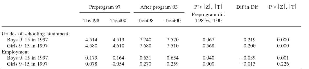
Differential exposure to Oportunidades: Schooling and work outcomes for households receiving benefits in 1998 versus 2000
Preprogram 97 After program 03 P⬎Z,T Dif in Dif P⬎Z,T
Treat98 Treat00 Treat98 Treat00
Preprogram dif. T98 vs. T00
Grades of schooling attainment
Boys 9–15 in 1997 4.514 4.513 7.740 7.520 0.967 0.219 0.000 Girls 9–15 in 1997 4.580 4.610 7.680 7.510 0.568 0.200 0.000 Employment
Boys 9–15 in 1997 0.179 0.164 0.631 0.654 0.040 ⳮ0.039 0.001
Girls 9–15 in 1997 0.078 0.054 0.270 0.259 0.000 ⳮ0.013 0.226
Table 4
Impact of Differential Exposure to Oportunidades on Schooling Grades and LFP Difference-in-difference Estimates: Adolescents 9–15 in1997, T1998 vs. T2000
Schooling Work
Coefficient 2003 level, Coefficient 2003 level, Standard By completed 1997 schooling [0.077]*** [0.025]
⬍⳱3 0.057 6.03, 0.9% ⳮ0.01 0.18,ⳮ5.5% By completed 1997 schooling [0.074]* [0.025]*
⬍⳱3 0.137 5.97, 2.3% ⳮ0.013 0.53,ⳮ2.5%
Behrman, Parker, and Todd 105
to three grades of schooling completed in 1997). The largest effects are observed for those who had completed five grades of schooling by 1997 (effects of 6.8 percent for girls, 4.4 percent for boys). The effects are most pronounced for those entering the last year of primary school at the time the program was introduced. In short, youth with 18 months greater exposure to the program accumulated significantly more schooling and this differential persisted for the longer-term five and a half-year period considered here. AnFtest rejects equality of coefficients at conventional significance levels for each set of subgroups (age and preprogram grades of school-ing) for both males and females, suggesting different impacts of PROGRESA/Opor-tunidades on schooling by age and preprogram schooling grades completed.
2. Impacts on Working15
The theoretical effect of PROGRESA/Oportunidades on the probability of working is ambiguous, as discussed in Section II. Over the short run, the program decreases working, but over the longer run, the program might increase working.16
In 1997 prior to the program, 0.18 of the T1998 boys and (significantly less at the 5 percent level) 0.16 of the T2000 boys were working; also, in 1997, 0.08 of the T1998 girls and (significantly less at the 1 percent level) 0.05 of the T2000 girls were employed (Table 3). Because of life-cycle work patterns, the proportions em-ployed in 2003 were much higher: for the T2000 boys 0.65 and for the T2000 girls 0.26 with obvious important gender differentials in work (Table 4). The DID estimate of the impact of the one and a half year differential exposure to the program on working five and a half years later (in 2003) shows that greater exposure significantly decreases the proportion working by 4.1 percent for boys with no significant effects for girls (Table 4). Effects do not significantly differ by age groups or by preprogram schooling level.
3. Do Effects Change Over Time?
The above impacts are based on beneficiaries who have received benefits about five and a half years versus nearly four years. An important policy issue is whether program impacts change over time. To analyze this, we add to our data the first round of the ENCEL evaluation survey that was carried out after the control group also began to receive benefits in 2000. Impact estimates for the year 2000 are based on comparing the treatment group which had two and a half years versus the control group at nearly a year of benefits. That is, we test whether impact estimates based on 2000 followup data are different from those based on the 2003 data used in this paper, allowing impact estimates to vary by evaluation round (2000 and 2003). Table
15. The definition of work excludes domestic work, which may underestimate the impacts of the program for girls. We do not analyze impacts on domestic work because we do not have baseline information. See Skoufias and Parker (2001) however for evidence suggesting that the program in the initial years reduced time spent in domestic work for girls.
Table 5
Do Oportunidades impacts change overtime? Experimental evidence comparing household treated in 1998 with households treated in 2000 (T1998 vs. T2000)
Year of impact
coefficient F test, Prob⬎F
2003 2000
Girls
All girls 9–15 in 1997 0.201 0.201 0.32 By age in 1997
9–10 0.075 0.057 0.63
11–12 0.181 0.234 0.43
13–15 0.32 0.313 0.21
By completed 1997 schooling grades
⬍⳱3 0.057 0.053 0.93
4 0.18 0.253 0.69
5 0.529 0.384 0.09*
6 0.304 0.28 0.19
7Ⳮ 0.117 0.21 0.33
Boys
All boys 9–15 in 1997 0.18 0.118 0.32
By age in 1997
9–10 0.197 0.123 0.52
11–12 0.241 0.094 0.39
13–15 0.139 0.135 0.95
By completed 1997 schooling grades
⬍⳱3 0.137 0.264 0.24
4 0.196 0.061 0.04**
5 0.347 0.075 0.02**
6 0.204 0.095 0.57
7Ⳮ 0.047 0.256 0.35
Notes: Estimates based on weighted DID regression estimates described in text. Controls for parental age, schooling, indigenous status, and housing characteristics (see text). * Significant at 10 percent; ** signifi-cant at 5 percent; *** signifisignifi-cant at 1 percent.
Behrman, Parker, and Todd 107
IV. Longer-Run PROGRESA/Oportunidades Impacts
after Five and a Half Years of Differential
Exposure
We now consider impacts based on a longer period of exposure to the program—that is, the five and a half year differential in program exposure, using DIDM estimates based on the new 2003 comparison group (Quadrant C) that was not exposed to the program. These estimates are useful for analyzing how longer program exposure might change impact estimates as well as studying variables such as work that are expected to have different impacts in the long run than in the short run. As an additional robustness check, we also estimate impacts comparing the original control group with the new comparison group, which provides estimates of differential exposure of about four years, impacts that should presumably be smaller for schooling than those based on five and a half years of differential exposure.
A. Data
The data used in this section are primarily from the 1997 ENCASEH and the EN-CEL2003. We link the ENCASEH97 to the ENCEL2003 to have longitudinal data on individual children who were aged 9–15 years in 1997 and aged 15–21 years in 2003. For the new C2003 comparison group households, we use recall data on their 1997 characteristics to characterize their eligibility status in 1997.17Using both the
2003 and 1997 rounds of data, we construct DIDM estimators of program impacts for the longer-run (five and a half years) impact of relatively large differences (four or five and a half years) in program exposure. For the schooling and work indicators, there are a total of 19,586 youth between the ages of 15 and 21 in 2003.
B. Methodology
To estimate the longer-run program impacts against the benchmark of no program with four or five and a half years difference in program exposure, we compare the original treatment groups (T1998 and T2000) with the new comparison group (C2003) that was drawn from rural areas that had not yet been incorporated into the program in 2003. Because the C2003 group was not selected randomly, we use matching methods to take into account differences in observed characteristics be-tween the T2000 and C2003 samples and bebe-tween the T1998 and C2003 sam-ples.18,19
17. Recall data from 1997 was only collected from the C2003 group and not from the T1998 and T2000 groups so that unfortunately we cannot judge the accuracy of the recall data compared with information collected on current characteristics in 1997. We carried out two exercises to insure our results are not biased by measurement errors in the recall data. 1) We compared average enrollment rates for youth aged 6–14 at the community level for T2000 and C2003 communities in the year 2000 and found similar patterns as to those for pre program education levels in our data in 1997 (based on recall data for C2003 and pre program surveys for T1998 and T2000). 2) We carried out alternative propensity score estimations using only current characteristics reported in 2003 and unlikely to have been affected by the program (such as parental education). The results are quite similar as to those presented.
The households living in localities where the program was not yet available were unlikely to have been affected by the existence of the program. However, because they lived in different geographic areas from the treatment sample, they may have experienced different local area effects (labor market conditions, quality of school-ing, prices) that also may be relevant determinants of outcomes of interest. To take such differences into account, we make use of DIDM estimators (Heckman, Ichi-mura, and Todd, 1997). The approach is analogous to the standard DID regression estimator, but does not impose functional form restrictions in estimating the condi-tional expectation of the outcome variable and reweights the observations according to the weighting functions implied by the matching estimators. We use local linear matching and bootstrapping to calculate standard errors for the main estimates pre-sented here.
The DIDM propensity score matching estimators are estimated in two stages. In the first stage, the propensity score is estimated using a logistic model and a set X consisting of preprogram (1997) household and locality level characteristics. The second stage uses local linear regression to construct matched no-treatment outcomes for each treated individual.
The variables used for the matching include demographic characteristics of the households in 1997, grades of schooling completed of household head and spouse in 1997, whether the household head and spouse spoke an indigenous language in 1997, whether the household head and spouse were employed in 1997, a number of household characteristics and consumer and production durables in 1997, the PRO-GRESA/Oportunidades’ poverty index score for program eligibility in 1997, income in 1997 and state of residence in 1997. Appendix Table A2 gives the estimated propensity score model for the T1998 to C2003 comparison, for which a Chi2test
indicates that the variables are jointly significant at the 0.1 percent level and have fairly good predictive power.20Figures 3 and 4 show the distributions of propensity
scores in the original treatment group (T1998) and the distribution of propensity scores in the C2003 comparison group. Although the distributions between the two groups for each comparison (that is, T2000 versus C2003 and T1998 versus C2003) are clearly different, there is adequate support in the sense that a number of house-holds in C2003 have propensity scores similar to those in T2000 and to those in T1998, although some comparison households with very high propensity scores are likely to be used a number of times as matches. To avoid matching children of
locality characteristics constructed using household information aggregated at the community level from the 1995 and 2000 Censuses on housing attributes, demographic structure, poverty levels, labor force participation, and ownership of durable goods. Selected localities were also constrained to come from the same states as the original 506 evaluation communities with the exception of one state where some com-munities from a neighbor state were used. All comcom-munities were constrained to satisfy PROGRESA/ Oportunidades eligibility characteristics with regard to distance to schools and health clinics. See Todd (2004) for further details.
19. Behrman, Parker, and Todd (2009b) analyze preprogram Census information on community charac-teristics between 1995 and 2000 for the evaluation sample, comparing T2000 and C2003. Those measuring schooling attainment show no significant differences between changes overtime in the T2000 and C2003 groups.
Behrman, Parker, and Todd 109
0
.5
1
1.
5
2
De
ns
it
y
0 .2 .4 .6 .8 1
Propensity score
Figure 3
Distribution of Propensity Score: Treatment 1998
different ages and genders, we implement the matching conditional on age and sex, as well as the household’s propensity score.
0
1
2
3
De
ns
it
y
0 .2 .4 .6 .8 1
Propensity score
Figure 4
Distribution of Propensity Score: New comparison group
C. Results
In this section, we present impact estimates on schooling, work and participation in agricultural work, comparing those with five and a half years of PROGRESA/Opor-tunidades to those never receiving benefits.21 For schooling, we also present
esti-mates based on the T2000 versus C2003 comparison—that is, estimating impacts for those with nearly four years of benefits versus never receiving benefits. This provides a benchmark against which to judge the reasonableness of the matching-based estimates; for a cumulative variable like schooling, program estimates should be larger for those with longer time exposure to the program.
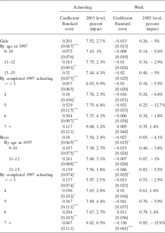
1. Impact on Schooling
Table 6 shows important effects on school grades completed for both boys and girls, particularly those who were younger when the program began. Boys aged 9–10 preprogram (15–16 in 2003) accumulate 1.0 additional grades of schooling than comparable boys without the program, while boys aged 11–12 preprogram
Behrman, Parker, and Todd 111
Table 6
Estimated Impacts of PROGRESA/Oportunidades on Grades of Schooling Local linear longitudinal DID matching † T1998 vs. C2003 and T2000 vs. C2003
C2003 Grades of schooling
T1998 versus C2003 T2000 versus C2003
Impact,
15–16 6.92 0.69 10.0 0.57 8.2
(0.16)*** (0.17)***
17–18 7.54 0.75 10.0 0.55 7.3
(0.18)*** (0.18)***
Notes: DIDM estimator, imposing common support (trimming⳱2 percent). Bootstrapped standard errors (parentheses) with 500 replications. Bandwidth⳱0.8.
mulate an additional 0.9 grades. Boys 13–15 preprogram accumulate about half a year of additional schooling. Impacts also are significant, although slightly smaller, for girls. Girls aged 9–12 preprogram accumulate 0.7 to 0.8 grades of schooling, with no significant impacts for older girls. Compared with schooling grades com-pleted of the comparison group in 2003 (about seven grades), these impacts represent significant increases of about 13–15 percent for boys and 10 percent for girls in overall schooling grades completed, relative to the comparison group never receiving benefits. Overall, the results show an important increase in schooling levels attained because of the program.
0
.2
.4
.6
.8
O
p
or
t i
m
pa
ct
s
1 2 3 4 5 6
Years with Oport
Coefficient estimate Upper CI Lower CI
Figure 5
Schooling impacts by program length: girls
exposure to the program than for those with shorter time of exposure, with impacts increasing in an approximately linear fashion with exposure.
2. Impact on Working
Behrman, Parker, and Todd 113
0
.2
.4
.6
.8
1
O
p
or
t i
m
pa
ct
s
1 2 3 4 5 6
Years with Oport
Coefficient estimate Upper CI Lower CI
Figure 6
Schooling impacts by program length: boys
3. Probability of Working in Agriculture
Schooling is often claimed to have higher returns in nonagricultural than in agri-cultural work, so if PROGRESA/Oportunidades were effective it might induce some shift out of the agricultural sector. We look at the unconditional probability of in-dividuals participating in agricultural work.22 Note that overall, girls have much
lower participation in agricultural work than boys. For boys, the reductions in ag-ricultural work for boys aged 9–10 preprogram are similar to the percentage reduc-tions in work, implying similar reducreduc-tions in agricultural as nonagricultural work (Table 7). For older boys—that is, aged 13–15 preprogram—however, on which there were no overall significant program effects on working, there are significant reductions in agricultural work, implying some substitution from agricultural work to nonagricultural work. For girls, there is no overall effect on participation in ag-ricultural work for younger girls, who also showed no effect on working. For older girls, for whom there was a significant increase in the probability of working, there is no significant increase in the probability of participating in agricultural work, again suggestive of increasing nonagricultural work.
Table 7
Estimated Impacts of PROGRESA/Oportunidades on Probability of Working and Participation in Agricultural Work Local linear longitudinal DID matching † T1998 vs. C2003
19–21 0.32 0.064 20.0 0.01 20.0
(0.038)* (0.02)
Notes: DIDM estimator, imposing common support (trimming⳱2 percent). Bootstrapped standard errors (parentheses) with 500 replications. Bandwidth⳱0.8. * Significant at 10 percent; ** significant at 5 percent; *** significant at 1 percent.
V. Benefit-Cost Estimates
The relatively large impacts on schooling attainment documented here raise the issue of whether the benefits of the PROGRESA/Oportunidades pro-gram justify the costs and in particular, how the propro-gram performs given its cost relative to other types of human capital programs. Clearly, PROGRESA/Oportuni-dades is not only a human capital investment program, because it also alleviates current poverty by giving money directly to the poor. Nevertheless, in this section, we offer a benefit-cost analysis of the program as if the only objective of the program were investment in human capital and the only benefits the subsequent impact on future earnings of the increased schooling attainment of students affected by PRO-GRESA/Oportunidades. Carrying out this analysis requires a number of additional assumptions and calculations, which are detailed below.
Behrman, Parker, and Todd 115
ignoring other potential impacts, such as that of improved health and nutrition. We estimate the return to schooling controlling for potential endogeneity using a plau-sible instrument given by a change in the compulsory schooling law in 1993 from sixth to ninth grade.23 The estimates are based on data from the 2002 nationally
representative Mexican Family Life Survey (MXFLS). We use the estimated returns to provide a guide for what the returns to schooling attainment for youth in rural areas are likely to be, and we also provide simulations based on varying levels of returns.
Focusing on the sample of men, a simple OLS estimate of returns to schooling attainment gives a value of 7.5 percent per year for this age group (16–24), which is similar across rural (7.2) and urban (7.6) areas. The IV estimate of wage functions increases the value to about 10 percent both for those residing in rural and in urban areas.24We provide simulations below based on 6 percent, 8 percent, and 10 percent
returns to schooling attainment.
The resource costs of the program include the administrative costs of the program (costs of transferring benefits, conditionality, and targeting) and the private costs associated with participation in the program.25The administrative and private costs
of participation in the program including the monetary and time costs of transpor-tation associated with greater school attendance were calculated in Coady (2000). He estimates that for each 100 pesos transferred, administrative and private costs are equivalent to 11.3 pesos. We assume that an additional year spent in school results in a 0.75 year decrease in time spent in the labor force.26We obtain estimates
other than transportation of the additional household expenses incurred because of increased schooling—that is, school supplies and children’s clothing—from an ear-lier study by Hoddinott, Skoufias, and Washburn (2000). Finally, for each peso of governmental expenditures (whether on resources or transfers) we assume a 25 per-cent increase in cost (grants plus administrative) from the distortions associated with raising revenues.27We assume that each youth in our sample receives the grants for
23. In 1993, lower secondary school (seventh through ninth grade) became mandatory. A main impact of this change was a large increase in the construction of lower secondary schools, the majority of which were of the telesecondary school type, which is a mode of secondary school provided only in rural areas. We use school construction interacted with whether an individual lived in rural areas at the age of 12 as a variable affecting completed schooling in 2002.
24. Similar increased estimated schooling effects with IV estimates are reported by Ashenfelter and Krue-ger (1994) for the United States, Duflo (2001) for Indonesia, and Behrman, Murphy, Quisumbing, and Young (2008) for Guatemala.
25. They do not include the budgetary costs of the schooling grants based on the calendar of grants (see Table 1) because these are transfers, not resource costs (see Knowles and Behrman 2004, 2005). An earlier study found no evidence of congestion costs or other spillover effects on nonbeneficiary students in the same schools, so we do not adjust for costs or benefits of spillovers either (Behrman, Sengupta, and Todd 2005).
six years. Youth in the absence of the program are assumed to begin working at age 18 and conclude at age 70.28All costs and benefits are discounted to time zero.
We assume a starting salary equal to the average obtained by youth aged 18 in the rural ENCEL areas of 2003, which is equal to $US163 monthly. This is a con-servative estimate of initial earnings opportunities as probably a number of youth will migrate to urban areas, where salaries tend to be higher. We use the schooling impacts on boys aged 15–16 (see Table 6).
Table 8 provides benefit-cost estimates of PROGRESA/Oportunidades, under the three different assumptions about the rate of return to schooling attainment (6, 8, and 10 percent) and three potential discount rates (3, 5, and 10 percent). Program benefits are several times higher than program costs under nearly all scenarios, with the exception of a very high discount rate and a low estimated return to schooling. Overall, then, even if the program were considered as only a human capital invest-ment program working only through increasing schooling attaininvest-ment, the overall benefits would seem to significantly outweigh the costs.
VI. Conclusions
This paper has provided a comprehensive analysis of longer-run pro-gram impacts of Oportunidades on schooling and work after five and a half years of program benefits. We have gone beyond previous studies of relatively short-term impact (two years or less) of limited differential program exposure (one and a half years at most) by investigating longer-run program effects of two types: (1) The impact of a short differential exposure on longer run outcomes (after five and a half years), estimated using treatment and control data from the large-scale randomized experiment, and (2) the impact of a longer (four or five and a half years) differential in exposure on longer-run outcomes, estimated using propensity score matching methods applied to data from the treatment group and from a nonexperimental com-parison group.
In summary, the longer-term impacts of the program appear quite positive with important increases in schooling attainment, and for older youth, some higher rates of working and a shift away from agricultural work to nonagricultural work. Benefit estimates based on earnings functions from adults integrated with careful costs es-timates indicate fairly high benefit-to-cost ratios unless the rate of return to schooling are low and the discount rate high. The additional years of data that we use, finally, permit much more confident inferences about longer-run effects. They suggest that (1) the initial differential exposure of one and a half years appears to have an impact on schooling attainment that is robust with the passage of time and (2) the program impacts on schooling attainment increase approximately linearly with the duration of exposure to the program.
Behrman,
Parker,
and
Todd
117
Table 8
Costs and Benefits of the PROGRESA/Oportunidades Program in U.S. dollars
Impact⳱1.0 grades of schooling Return to schooling
Initial Earnings 6% 8% 10%
Discount rate
Without
program With program Costs Benefits B/C Ratio Benefits B/C Ratio Benefits B/C Ratio
3% 1,855 1,966 500 1801 3.60 2,679 5.36 3,557 7.11 5% 1,855 2,003 390 664 1.70 1,082 2.77 1,499 3.84 10% 1,855 2,040 215 27 0.13 233 1.08 438 2.04
Impact⳱0.83 grades of schooling
Initial Earnings 6% 8% 10%
Discount rate
Without
program With program Costs Benefits B/C Ratio Benefits B/C Ratio Benefits B/C Ratio
3% 1,855 1,966 500 1,502 3.00 2,231 4.46 2,959 5.92 5% 1,855 2,003 390 556 1.43 903 2.32 1,245 3.19 10% 1,855 2,040 215 28 0.13 198 0.92 363 1.69
Notes: Calculations assume youth take part in the program for six years, beginning at age 10 and finishing at age 16. A return to experience is included⳱
Behrman, Parker, and Todd 119
Appendix
Table A1
Probability of attriting between 1997–2003 by 1997 characteristics: T1998 vs. T2000 Girls and Boys 9–15 program eligible in 1997
All attritors Boys Girls
Treatment⳱1 0.016 ⳮ0.021 0.012 ⳮ0.015 0.02 ⳮ0.06 T1998⳱1, T2000⳱0 [0.01]*** [0.088] [0.008] [0.121] [0.008]** [0.128] Interactions
Treatment*age ⳮ0.003 0 ⳮ0.007
[0.006] [0.008] [0.009]
Treatment*gender ⳮ0.029
[0.016]*
Treatment*indigenous ⳮ0.04 ⳮ0.047 ⳮ0.026
[0.034] [0.047] [0.050]
Treatment*schooling 0.005 ⳮ0.003 0.013
[0.005] [0.007] [0.008]*
Treatment*enrolled 0.056 0.072 0.043
[0.022]** [0.031]** [0.031]
Treatment*father schooling 0.002 0.002 0.002
[0.004] [0.006] [0.006]
Treatment*father age 0.002 ⳮ0.001 0.005
[0.001] [0.002] [0.002]**
Treatment*father indig. 0.176 0.11 0.25
[0.065]*** [0.090] [0.091]*** Treatment*father bilingual ⳮ0.114 ⳮ0.06 ⳮ0.172
[0.052]** [0.074] [0.074]**
Treatment*mother schooling ⳮ0.004 ⳮ0.001 ⳮ0.008
[0.004] [0.006] [0.006]
Treatment*mother age ⳮ0.001 0.001 ⳮ0.004
[0.002] [0.002] [0.002]
Treatment*mother indig ⳮ0.069 ⳮ0.032 ⳮ0.121
[0.047] [0.065] [0.068]*
Treatment*mother bilingual 0.067 0.02 0.12
[0.037]* [0.050] [0.053]**
Treatment*rooms 0.005 0.002 0.007
[0.009] [0.012] [0.013]
Treatment*electricity ⳮ0.021 ⳮ0.034 ⳮ0.008
[0.018] [0.025] [0.027]
Treatment*water 0.009 0.045 ⳮ0.026
[0.019] [0.027]* [0.027]
Treatment*dirt floor ⳮ0.016 ⳮ0.027 ⳮ0.002
[0.019] [0.027] [0.028]
Observations 16,257 16,117 8,384 8,311 7,870 7,806
Table A2
Logit Model for Probability of Participating in Rural PROGRESA/Oportunidades
Variable Coefficient Standard Error
Variable Coefficient Standard Error
Age of household head 0.002 1.640 Total household income squared
0.000 0.000
Age of spouse ⳮ0.004 0.003 Blender ⳮ0.011 0.052
Gender of household head 0.644 0.090 Refrigerator 0.183 0.091 Household head speaks
indigenous language
0.274 0.066 Gas stove 0.576 0.065
Spouse speaks indigenous language
0.267 0.072 Gasheater 0.250 0.129
Grades of schooling household head
ⳮ0.058 0.008 Radio 0.109 0.035
Grades of schooling spouse
ⳮ0.129 0.009 Television 0.15 0.043
Employed household head ⳮ0.542 0.075 Video 0.304 0.142
Employed spouse ⳮ0.445 0.054 Washer 0.603 0.154
Children 0–5 ⳮ0.393 0.023 Car ⳮ0.098 0.177
Children 6–21 ⳮ0.265 0.024 Truck 0.048 0.126
Children 13–15 0.036 0.030 State1 1.144 0.116
Children 16–20 0.060 0.024 State2 0.630 0.080
Women 20–39 0.086 0.058 State3 0.768 0.084
Women 40–59 ⳮ0.104 0.048 State4 0.341 0.080
Women 60Ⳮ ⳮ0.379 0.045 State5 0.382 0.080
Men 20–39 0.021 0.038 State6 ⳮ0.463 0.075
Men 40–59 ⳮ0.495 0.050 Missing grades of schooling household head
ⳮ2.156 0.080
Men 60Ⳮ ⳮ0.727 0.056 Missing grades of schooling spouse
ⳮ2.352 0.116 Number of Rooms 0.238 0.020 Missing age household head 0.937 0.853 Electricity in HH ⳮ0.242 0.04 Missing age spouse ⳮ0.836 1.321 Water in HH ⳮ0.367 0.039 Missing indig household
head
1.974 1.387
Dirt floor ⳮ0.583 0.048 Missing working household head
1.045 2.219
Room material (inferior) 0.197 0.043 Missing working spouse 1.087 0.409 Wall material (inferior) 0.135 0.046 Missing water ⳮ0.336 0.468 Own animals 0.198 0.040 Missing electricity 0.404 0.522
Own land 0.223 0.037 Missing rooms 0.371 0.345
Oportunidades score 1997 1.632 0.108 Missing income ⳮ2.203 0.762 Score squared ⳮ0.115 0.015 Missing ownanimals ⳮ0.609 0.534 Total HH income 0.000 0.000 Missing ownland 0.824 0.523
Constant ⳮ1.658 0.242
Number of observations 13,336
LR chi2(60) 10,591 Pseudo R2 0.584
Behrman, Parker, and Todd 121
References
Ashenfelter, Orley, and Alan Krueger. 1994. “Estimates of the Economic Return to Schooling from a New Sample of Twins.”American Economic Review84(5):1157–74. Ballard, Charles, John Shoven, and John Whalley. 1985. “General equilibrium computations
of the marginal welfare costs of taxes in the United States.”American Economic Review 75(1):128–38.
Banerjee, Abhijit, Shawn Cole, Esther Duflo, and Leigh Linden. 2007. “Remedying education: evidence from two randomized experiments in India.”Quarterly Journal of Economics122(3):1235–64.
Behrman, Jere. 2009. “Investment in Education-Inputs and Incentives.” InHandbook of Development Economics: The Economics of Development PolicyVol. 5 ed. Rodrik Dani and Mark R. Rosenzweig, 4883–4975. Amsterdam: North-Holland Publishing Co. Behrman, Jere, Alexis Murphy, Agnes Quisumbing, and Kathryn Young. 2009. “Are
Returns to Mothers’ Human Capital Realized in the Next Generation? The Impact of Mothers’ Intellectual Human Capital and Long-Run Nutritional Status on Child Human Capital in Guatemala.” IFPRI Discussion Paper 850. Washington, D.C.: International Food Policy Research Institute.
Behrman, Jere, Susan Parker, and Petra Todd. 2009a. “Medium-Term Impacts of the AmericanOportunidadesConditional Cash Transfer Program on Rural Youth in Mexico.” InPoverty, Inequality, and Policy in Latin America, Ed. Klasen Stephan and Nowak-Lehmann Felicitas, 219–70. Cambridge: MIT Press
Behrman, Jere, Susan Parker, and Petra Todd. 2009b. “Schooling Impacts of Conditional Cash Transfers on Young Children: Evidence from Mexico.”Economic Development and Cultural Change57(3):439–78.
Behrman, Jere, Piyali Sengupta, and Petra Todd. 2005. “Progressing Through PROGRESA: an Impact Assessment of a School Subsidy Experiment.”Economic Development and Cultural Change54(1):237–76.
Bobonis, Gustavo, and Frederico Finan. 2009. “Neighborhood Peer Effects in Secondary School Enrollment Decisions.”Review of Economics and Statistics91(4):695–716. Cameron, Stephen, and James Heckman. 2008. “Life Cycle Schooling and Dynamic
Selection Bias: Models and Evidence for Five Cohorts of American Males.”Journal of Political Economy106(2):262–333.
Coady, David. 2000. “The Application of Social Cost-Benefit Analysis to the Evaluation of PROGRESA.”Final Report. Washington, D.C.: International Food Policy Research Institute.
Dehejia, Rajeev, and Sadek Wahba. 2002. “Propensity Score Matching Methods for Nonexperimental Causal Studies.”Review of Economics and Statistics84(1):151–61. Duflo, Esther. 2001. “Medium Run Effects of Educational Expansion: Evidence from a
Large School Construction Program in Indonesia.”American Economic Review 91(4):795–813.
Feldstein, Martin. 1995. “Tax Avoidance and the Deadweight Loss of the Income Tax.” National Bureau of Economic Research Working Paper No. 5055. Cambridge, Mass. Glewwe, Paul, and Michael Kremer. 2006. “Schools, Teachers, and Education Outcomes in
Developing Countries.” In:Handbook of the Economics of Education vol. 2ed. Hanushek Eric and Finis Welch. Amsterdam: Elsevier Press.
Harberger, Arnold. 1997. “New Frontiers in Project Evaluation? A Comment on Devarajan, Squire and Suthiwart Narueput.”The World Bank Research Observer12(1):73–79. Heckman, James, Hidehiko Ichimura, and Petra Todd. 1997. “Matching as an Econometric
Hoddinott, John, Emmanuel Skoufias, and Ryan Washburn. 2000. “The Impact of PROGRESA on Consumption.”Final Report. Washington, D.C.: International Food Policy Research Institute.
King, Elizabeth, and Jere Behrman. 2009. “Timing and Duration of Exposure in Evaluations of Social Programs.”World Bank Research Observer24(1):55–82.
Knowles, John, and Jere Behrman. 2004. “A Practical Guide to Economic Analysis of Youth Projects.” Washington, D.C.: World Bank.
Knowles, John, and Jere Behrman. 2005. “Economic Returns to Investing in Youth.” inThe Transition to Adulthood in Developing Countries: Selected Studies, ed. Jere Behrman, Barney Cohen, Cynthia Lloyd, and Nelly Stromquist 424–90. Washington, D.C.: National Academy of Science-National Research Council.
Miguel, Edward, and Michael Kremer. 2004. “Worms: Identifying Impacts on Education and Health in the Presence of Treatment Externalities.”Econometrica72(1):159–217. Orazem, Peter, and Elizabeth King 2008. “Schooling in Developing Countries: The Roles of
Supply, Demand and Government Policy.” In:Handbook of Development Economics, Vol. 4, ed. T. Paul Schultz and John Strauss 3475–3560. Amsterdam: North-Holland
Publishing Co.
Parker, Susan, Luis Rubalcava, and Graciela Teruel. 2008. “Evaluating Conditional Schooling-Health Transfer Programs.” In:Handbook of Development Economics, Vol. 4, ed. T. Paul Schultz and John Strauss 3963–4035. Amsterdam: North-Holland Publishing Co.
Ravallion, Martin, and Quentin Wodon. 2000. “Does Child Labor Displace Schooling? Evidence on Behavioral Responses to an Enrollment Subsidy.”Economic JournalRoyal Econometric Society 110(462):158–75.
Rosenbaum, Paul, and Donald Rubin. 1985. “Constructing a Control Group Using Multivariate Matched Sampling Methods that Incorporate the Propensity Score.” American Statistician3:33–38.
Schultz, T. Paul. 2004. “School Subsidies for the Poor: Evaluating a Mexican Strategy for Reducing Poverty.”Journal of Development Economics74(1):199–250.
Skoufias, Emmanuel, and Susan Parker. 2001. “Conditional Cash Transfers and their Impact on Child Work and Schooling: Evidence from the PROGRESA program in Mexico.” Economia2(1):45–96.
Todd, Petra. 2004. “Technical Note on Using Matching Estimators to Evaluate the Opportunidades Program For Six Year Followup Evaluation of Oportunidades in Rural Areas. Philadelphia: University of Pennsylvania. Unpublished.
Todd, Petra, and Jeff Smith. 2005. “Does Matching Overcome LaLonde’s Critique of Nonexperimental Estimators.”Journal of Econometrics125(1–2):305–53.