UNDERSTANDING TAX EVASION DYNAMICS
Eduardo M. R. A. Engel James R. Hines Jr.
SERIE ECONOMIA No 47
Diciembre, 1998
Centro de Econom´ıa Aplicada Departamento de Ingenier´ıa Industrial Facultad de Ciencias F´ısicas y Matem´aticas
Universidad de Chile
Understanding Tax Evasion Dynamics
By Eduardo M. R. A. Engel and James R. Hines Jr.1
December 1998
Abstract
Americans who are caught evading taxes in one year may be audited for prior years. While the IRS does not disclose its method of selecting tax returns for audit, it is widely believed that a taxpayer’s probability of being audited is an increasing function of current evasion. Under these circumstances, a rational taxpayer’s current evasion is a decreasing function of prior evasion, since, if audited and caught evading this year, the taxpayer may incur penalties for past evasions. The paper presents a model that formalizes this notion, and derives its implications for the responsiveness of individual and aggregate tax evasion to changes in the economic environment. The aggregate behavior of American taxpayers over the 1947-1993 period is consistent with the implications of this model. Specifically, aggregate tax evasion is higher in years in which past evasions are small relative to current tax liabilities - which is the case when incomes or tax rates rise. Furthermore, aggregate audit-related fines and penalties imposed by the IRS are positively related not only to aggregate current-year evasion but also to evasion in prior years. The estimates imply that the average tax evasion rate in the United States over this period is 42% lower than it would be if taxpayers were unconcerned about retrospective audits.
JEL Classification: H26, K42.
Keywords: Aggregate tax evasion, retrospective audits, tax amnesties.
1
1
Introduction
The U.S. tax system relies on a form of voluntary compliance. Under U.S. law, taxpayers are required to assist tax authorities by reporting their incomes honestly and paying taxes based on their reported incomes. The system is actively enforced by the Internal Revenue Service (IRS) and the courts, who can impose substantial penalties for noncompliance. Nevertheless, tax evasion is a major concern in the United States, and even more so in other countries.2 Individuals underreport approximately 10.6% of their incomes annually in the United States, and the IRS estimates that tax evasion reduces U.S. tax collections by $190 billion annually (Herman, 1998). Little is understood about the factors that determine how much income individuals report to the government and, of particular interest to policymakers, about the way in which aggregate compliance responds to changes in the economic and policy environment.
This paper analyzes a feature of tax enforcement that encourages a particular dynamic tax evasion pattern in the United States. The IRS is careful not to disclose its audit policies, but there is some consensus within the taxpaying public about various aspects of its practices. Tax returns are selected for examination in an initial pass, and if not chosen within a period of about a year, a return is very unlikely to be examined later unless some unusual event draws the IRS’s attention to it. U.S. law provides statutes of limitations — three years for minor tax evasions and six years for major tax evasions. The determinants of whether a return will be audited are not known with certainty, but the audit probability is widely believed to be a function of the extent to which a taxpayer underreports income in the current year. Under these circumstances, a taxpayer who evades much of his tax liability in one year has an incentive to report honestly in the following year, since, if he is subsequently audited and caught evading, he is at greater risk of incurring substantial penalties for past evasions.
Section 2 of the paper formalizes this notion by introducing a model of tax evasion in which taxpayers who were not audited during the previous year are conscious of their potential liabilities for undiscovered past evasions. As a general matter, these taxpayers are likely to evade less this year if last year’s evasion level was particularly high, and conversely, to evade more than usual following a year of little evasion. These general tendencies are tempered somewhat by the dynamic nature of any taxpayer’s compliance problem. Higher-than-normal evasion in a year following little
2The paper uses the term “evasion” to include not only fraudulent evasion but also other forms of willful income
evasion makes sense, but imposes some costs on a taxpayer in the subsequent year, when evasion becomes more costly since more is at risk. The cumulative incentives facing individual taxpayers become somewhat complicated functions of past evasion behavior and expected future variables.
It is possible for the dynamic behavior of aggregate evasion to differ substantially from the behavior of any individual taxpayer. Individuals may alternate years of high evasion followed by low evasion. If, however, two individuals evade taxes in cycles perfectly out of phase with each other, with one evading a large amount while the other evades little, then their aggregate behavior may not be cyclical at all.
Aggregate tax evasion behavior will, however, show predictable cyclical patterns in the presence of observable aggregate economic shocks that influence most taxpayers. For example, tax evasion rates are likely to fall during recession years, since most taxpayers find that their stocks of past (and yet undiscovered) evasions loom large relative to their (reduced) current incomes. Tax rate changes and changes in enforcement efforts generate analogous aggregate responses. Section 3 presents calculations of the aggregate responses of taxpayers to changes in the general economic environment.
Section 4 of the paper examines aggregate tax enforcement and compliance behavior in the United States over the 1947-1993 period. The evidence is consistent with the important aspects of the model of tax evasion dynamics analyzed in sections 2-3. One feature of the model is that audits include retrospective examination of the tax returns of individuals caught evading. While it is not possible to check this specification directly, annual fines and penalties imposed by the IRS subsequent to audits are positively correlated with contemporaneous and several lags of tax evasion as calculated from national income account statistics.
The model implies that positive changes in tax rates and income growth stimulate greater evasion (as a fraction of income), while higher tax enforcement intensity discourages evasion. The regressions indicate that the level of aggregate tax evasion, and changes in the level of evasion, respond to aggregate variables in a manner that is consistent with these predictions. Specifically, tax evasion appears to rise and then fall in response to positive shocks to income. Similarly, lagged tax evasion is negatively correlated with current tax evasion after controlling for other changes in the economic environment.
the United States is 42% lower than it would be if taxpayers were not conscious of their uncaught past evasions when reporting their current incomes to the government. Another implication of the estimated parameters is that doubling the current penalty rate from 25 to 50% would reduce the average evasion rate by only 8%. The model implies as well that any tax revenue gains associ-ated with tax amnesties are likely to be short-lived, as taxpayers participating in amnesties have incentives to raise their subsequent evasion rates since they have less to hide from the government. Section 6 is the conclusion.
2
A Model of Tax Evasion Dynamics
This section presents a tax evasion model in which undiscovered past tax evasion influences current behavior. In the interest of expositional clarity, the model simplifies certain aspects of the legal and economic environment.
2.1 The Basic Framework
The model considers cases in which individuals choose the fraction of income they report to the IRS while facing stochastic probabilities of being audited. If individuals are caught evading taxes this year the IRS examines their tax returns for the previous year as well.3 In this simple specification of the model, unreported income is either discovered by an IRS audit in the year that follows the tax filing, or is discovered when the taxpayer is audited and caught evading the following year, or else is never discovered.4
Taxpayers are risk-neutral, and therefore select evasion strategies that minimize the expected
3
The assumption that retrospective audits are limited to only one previous year simplifies the derivations but can easily be relaxed. Under U.S. law, there is a three-year statute of limitations for government prosecutions of “small” evasions (underreportings of 25% or less of Adjusted Gross Income), a six-year statute of limitations for “large” evasions, and no statute of limitations for prosecutions of tax fraud. This issue is discussed at length in section 4.
4This specification of IRS behavior is consistent with the description of Sprouse (1988) and others of how the
discounted sum of tax payments and penalties.5 Using yt to denote true income in year t, an individual chooses to reportdtof income to the government, leaving an amount (yt−dt) unreported. The evasion rate is the fraction of income not declared to the tax authorities; it is denoted et ≡ (yt−dt)/yt. For simplicity, taxes are taken to be linear functions of income at rateτt in period t. Then an individual’s self-reported tax liability is: τtdt =τtyt(1−et), which excludes the obligation a taxpayer faces if caught cheating by the government.
The probability that an individual is audited is an increasing function of the current evasion rate.6 In addition, the audit probability is a function of the enforcement efforts of the IRS. The functionπ(pt, et) indicates the probability that an individual’s tax return will be selected for audit, in whichptdenotes the intensity of enforcement efforts and et the individual’s evasion rate. In the notation that follows, this function is often represented in the simplified form πt(et), the subscript tto the π function denoting that variables outside of an individual’s control are held constant.7
Individuals who are audited and caught evading their taxes incur several costs. The first is the burden of repaying with interest past taxes due plus penalties charged by the IRS on unreported income discovered by audits.8 Other costs include the pecuniary and psychological costs of enduring audits and court trials, as well as prison time or other sanctions imposed on individuals found guilty of major crimes. Of these, the model incorporates only the first. Criminal penalties such as prison
5
This formulation is chosen in order to focus the model on the dynamic issues raised by the ability of the government to discover past undeclared income. The implications of the model used here generalize naturally to cases in which individuals exhibit risk aversion of a type considered in other studies.
6As in Reinganum and Wilde (1985), Border and Sobel (1987), Scotchmer (1987), Yitzhaki (1987), S´anchez and
Sobel (1993), and Cremer and Gahvari (1994). Andreoni et al. (1998) survey this literature. There is lively speculation about the algorithm used by the government to select tax returns for audit, much of the speculation fueled by the unwillingness of the IRS to reveal anything about its screening methods. See, for example, Burnham (1989). The model assumes that the IRS does not use past information (including an individual’s audit history) in selecting returns to audit this year — a specification that is consistent with information from various sources indicating that, until very recently, the IRS technology made it impossible for them to use the results of past audits as criteria in selecting returns for new audits. (This limitation did not prevent the IRS from examining earlier returns of taxpayers in the course of audits in subsequent years.) The model and empirical work that follows assume that tax evasion takes the form of underreporting income rather than overclaiming tax credits, claiming too many exemptions, or using other tactics. The model also ignores the fact that sources of income differ in the ease with which taxpayers can successfully underreport income to the IRS without being caught — though incorporating such income heterogeneity would change the model very little.
7
Here and elsewhere, annual incomeytis taken to be unaffected by levels of tax enforcement and individual evasion decisions. Of course, in a general model in which individuals simultaneously work, save, and evade taxes, changes in the intensity of tax enforcement, and changes in the penalties for tax evasion, may influence individual decisions of how much income to earn. These issues are examined by Weiss (1976), Pencavel (1979), Sandmo (1981), Cowell (1985), and Mayshar (1991), but are not incorporated in the model that follows.
8
terms are very seldom imposed on tax evaders other than those who are significant criminal figures.9 If caught evading taxes, an individual must pay with corresponding interest the amount owed plus a penalty that is generally equal to 25 percent of the previously unpaid tax liability. This penalty rate,10 which has stayed roughly constant over time, influences an individual’s incentives to report income to the IRS; we use a time-invariant parameter,α, to denote the penalty rate.
In selecting the amount of income to report in one year, an individual who seeks to minimize the present discounted value of lifetime tax liabilities must incorporate the impact of this year’s evasion on all future tax liabilities. Consider the case of an individual with τt−1et−1yt−1 of undiscovered tax liabilities for year t−1. We denote by Vt(et−1) the individual’s expected discounted present value, as of periodt, of all future tax liabilities as a function of aggregate variables such as income, enforcement intensities (summarized in thetsubscript), and the stock of potential liability for year (t−1)’s evaded taxes carried forward to periodt. By Bellman’s principle, Vtsatisfies:11
Vt(et−1) = mine
in whichrt−1 denotes the interest paid on unreported period (t−1) income caught by the IRS in periodt, and the parameter β is the individual’s one-period subjective discount factor. The right hand side terms of (1) have the following interpretation: The first term denotes tax payments in periodt before any audits take place, as a function of the level of evasion chosen by the taxpayer for that period. The second term is expected tax payments as of period (t+ 1), appropriately discounted, conditional on not having been audited in periodt. The expectations operator applies to variables unknown at time t, such as future income and tax rates. The third term describes what happens when the taxpayer is audited in period t: penalties and interest on all evasion in years t and (t−1) must be paid, and future tax liabilities now are evaluated taking into account that there will be no evasion carried into the next period.
9
The 1975 Annual Report of the Commissioner of Internal Revenue reports that, over the 1971-1975 period, a yearly average of 1,042 individuals were convicted of criminal tax fraud. This figure represents 0.0013% of the roughly 80 million individuals who filed tax returns each year over that period.
10Strictly speaking, there are more than 100 different penalties that can be applied to tax returns that are negligent,
fraudulent, frivolous, contain substantial valuation errors, understatements of tax liabilities, or other defects. Penalty rates depend on the nature and severity of the infraction. The 25 percent figure characterizes the common practice in serious cases.
11
Equation (1) illustrates the importance of the dynamic considerations in the taxpayer’s choice of evasion level. If taxpayers who are caught evading in one year are never investigated for their behavior in the previous year, then Vt+1 is a constant and the first order condition becomes:
1
1 +α =πt+etπ
′
t(et). (2)
Equation (2) has certain well-known properties, including the feature that the tax rate and the level of income have no impact on the evasion rate, as long as the π function takes the form assumed in its specification as πt(et). The reason is that the return to evading and the penalty for being caught evading are both homogeneous of degree one in income and the tax rate, so the marginal condition that characterizes optimal evasion behavior as a fraction of total income is unaffected by income and tax rate changes. A number of earlier tax evasion studies examine the impact of risk aversion in the consumer’s utility function, in part because risk aversion can introduce correlations between the fraction of income evaded and tax rates and income.12 Of course, even in the formulation of the static model with concave utility, last period’s evasion level does not influence this year’s evasion decision.
2.2 Retrospective Enforcement
The following analysis considers the implications of the dynamic problem specified in (1), at times contrasting them with the more standard implications of (2). The purpose is to identify properties of the value function and the implied evasion behavior of rational taxpayers. The results establish conditions under which a unique, increasing, concave, and differentiable value function exists. Fur-thermore, under these conditions, the implied evasion correspondence is single-valued, decreasing, continuous, and decreasing in past evasion. These properties reinforce economic intuition concern-ing the effects of retrospective auditconcern-ing, and provide the foundation for the simulations and data analysis that follow.
In order to prove formal results, and to compute expressions for value functions and optimal policies, it is necessary to make assumptions on taxpayers’ expectations about the future values of
12
interest rates, income growth, tax rates and enforcement behavior by the IRS. We assume that the preceding variables remain constant (and that taxpayers are aware of this). Toward the end of this section we consider the case where these parameters may change.
Denoting Wt(et−1)≡Vt(et−1)/τtyt, our assumptions on the evolution of future variables imply thatWt does not depend ont. It follows from dividing both sides of (1) byτtyt that
W(et−1) = mine
n
(1−e) + β(1 +g)(1−π(e))W(e) (3)
+π(e) [(1 +α) (e+xet−1) +β(1 +g)W(0)] o
,
in whichx≡(1+r)/(1+g), withgdenoting the growth rate ofτ y, i.e.,g≡[(τtyt−τt−1yt−1)/τt−1yt−1]. The time subscript is omitted fromπ(e) in (3), since the audit function is unchanging. The variable x captures the extent to which income growth and tax changes affect the relative importance of evasion rates in adjacent periods.
The following proposition shows that the problem characterized by (3) has a well defined solu-tion.
Proposition 2.1 Assume β(1 +g) < 1. Then there exists a unique function W solving (3). Furthermore, this function is continuous.
Proof The proof is a direct application of Blackwell’s Theorem. See Appendix C.
Associated with the solution of (3) there is a policy correspondence that associates with every past evasion rateet−1 a set of evasion rates at which the minimum of the right hand side of (3) is attained. This correspondence is denoted by Φ(et−1). It is non-empty since a continuous function attains a minimum over a compact set.
It follows from (3) that W does not directly depend on τ. Hence the evasion correspondence Φ (and the eventual policy function) do not depend on the tax rate either. The value functionW and the evasion correspondence Φ depend, instead, on the growth rate of tax liabilities,g, and the factor xthat captures the importance of past evasion relative to current income. Small values of x indicate that past evasion is relatively small compared with current income, so that the individual is likely to choose a higher current evasion rate. The value and evasion functions also depend on the discount rate β, the penalty rate α, and the audit function π.
a taxpayer is subject to penalties that are proportional to amounts evaded. Since the taxpayer selects the level of current evasion bearing in mind the potential penalties if caught, it follows that W is concave rather than linear in et−1.
Proposition 2.2 The value function is increasing and concave. Furthermore, it is strictly
increas-ing at all points et−1 where π(e)>0 for all e∈Φ(et−1).
Proof The following notation will be useful throughout many of the proofs that follow:
A(e) ≡ 1−e+β+(1−π(e))W(e) +π(e)[(1 +α)e+β+W(0)], (4)
B(e) ≡ (1 +α)xπ(e), (5)
in which β+≡β(1 +g). The functionB(e) reflects the expected tax liability (including penalties) for each dollar of past evasion at risk of being uncovered by audits this year, whileA(e) reflects the expected present value of all other current and future tax liabilities. Bellman’s equation (3) may then be written as:
W(s) = min
0≤e≤1{A(e) +B(e)s}. (6)
Since G(e, s)≡A(e) +B(e)sis linear ins, it follows that, forλ,e1,t−1 and e2,t−1 in [0,1]:
G(e, λe1,t−1+ (1−λ)e2,t−1) =λG(e, e1,t−1) + (1−λ)G(e, e2,t−1). (7)
Note that for any pair of real valued functions f1 and f2 defined on a compact subset of the real line
min
e [f1(e) +f2(e)]≥[mine f1(e)] + [mine f2(e)]. (8)
It follows that taking the minimum on both sides of (7) demonstrates that W is (weakly) concave. Next it is shown that W is increasing. The following inequality is useful to prove this (and other) results. Given y in [0,1] then for allz in [0,1] and all φy in Φ(y):
W(y)≥W(z) +B(φy)(y−z). (9)
= A(φy) +B(φy)z+B(φy)(y−z)
≥ min
e {A(e) +B(e)z}+B(φy)(y−z) = W(z) +B(φy)(y−z).
To show thatW is increasing, lety > z and φy ∈Φ(y). Then, from (9) it follows that
W(y)≥W(z) +B(φy)(y−z).
SinceB(φy)≥0, with strict inequality if π(φy)>0, this implies the monotonicity result forW. The following proposition shows that the optimal evasion rate decreases with past evasion.
Proposition 2.3 The correspondence Φ is (weakly) decreasing. That is, if φ1 ∈ Φ(s1) and φ2 ∈ Φ(s2), with s1 < s2, then φ2 ≤φ1.
Proof Applying (9) withs1 in the place of y and s2 in the place of z,
W(s1)≥W(s2) +B(φ1)(s1−s2).
And applying (9) withs2 in the place ofy and s1 in the place of z,
W(s2)≥W(s1) +B(φ2)(s2−s1).
From these two weak inequalities it follows that
W(s1) +B(φ2)(s2−s1)≤W(s2)≤W(s1) +B(φ1)(s2−s1).
Ass2 > s1, it follows that
B(φ2)≤B(φ1).
And since B is increasing — which follows from assuming that π is increasing — it must be the case that φ2≤φ1.
past have incentives to increase their evasion rates. The steady state of this process is the evasion rate chosen by a taxpayer after a large number of years without being subject to an audit. It is convenient to refer to this as the “conditional steady state evasion rate,” or “conditional long-run evasion rate” and denote it bye∗.13
Since the policy correspondence is weakly decreasing, whenever it takes more than one value at a point the correspondence is discontinuous, and the conditional steady-state need not exist. The following proposition provides sufficient conditions for the policy correspondence to be single-valued. It is followed by a proposition showing that, under these conditions, the policy function is continuous. The existence of the conditional steady-state then follows directly.14
Proposition 2.4 Assumeπ is strictly increasing, convex, twice differentiable, with bounded second
derivative. Furthermore, suppose the following inequality holds:15,16
[(1 +x)π′(1) + (1 +βx)π(1)e
−βxπ(0)e 2]≤ 1 1 +α. Then Φis single-valued.
Proof The proof is rather long and cumbersome, and therefore relegated to Appendix E.
In what follows, the policy function associated with Φ is denoted by φ. As mentioned earlier, φ does not depend on the tax rate but does vary withg,x,β,αandπ. It follows from Proposition 2.2 thatφ is (weakly) decreasing and, from the following proposition, that it is continuous.
Proposition 2.5 Under the assumptions of the preceding proposition the policy function is
con-tinuous.
Proof Since Φ is single valued, it suffices to prove upper hemicontinuity of Φ. And since Φ(s) is a subset of the unit interval, this is equivalent to showing that Φ has a closed graph. Thus, consider
13
It should be noted that a particular taxpayer’s evasion rate is unlikely to converge toe∗, since every year there is a probability of being audited, discovered, and starting the following year with no undiscovered past evasions. This is the reason for the “conditional” qualifier.
14
This amounts to saying that a continuous function from [0,1] to [0,1] has a fixed point, which holds trivially. And since the policy function is strictly decreasing, this fixed point is unique.
15
Forπ(e) =peγ, withγ≥1, the following condition simplifies to: [(1 +x)γ+ (1 +βxe )]π(1)≤ 1
a sequence sn that converges to ¯s, and a sequence yn∈Φ(sn) that converges to ¯y; for the proof it is sufficient to show that ¯y∈Φ(¯s).
From yn∈Φ(sn) it follows that for alle∈[0,1]:
A(yn) +B(yn)sn≤A(e) +B(e)sn,
with A and B defined in (4) and (5). And since A and B are continuous,17 taking the limit as n tends to infinity implies that, for alle∈[0,1]
A(¯y) +B(¯y)¯s≤A(e) +B(e)¯s.
Thus ¯y ∈Φ(¯s).
Some basic properties of the dynamic problem follow directly from the Bellman equation (3) once it is shown that the value function is differentiable. For example, the envelope theorem then implies that:
W′(e
t−1) = (1 +α)π(et)x, (10)
in which W′(
·) denotes the derivative of W. Equation (10) implies that the present value of expected tax payments beginning this period, and including fines on last period’s evasion, increases with the amount evaded last period. The increase equals the product of the additional fine the individual must pay if audited and the probability of being audited.
The following proposition provides conditions under which (10) holds.
Proposition 2.6 Under the assumptions of Proposition 2.4 the value function has a continuous
derivative given by (10).
Proof It follows from (9) thatB(φ(s)) is a subgradient forW ats. SinceW is concave (Proposi-tion 2.2), Corollary 24.2.1 in Rockafeller (1970, p. 231) implies that:
W(s)−W(0) =
Z s
0
B(φ(u))du.
And as B(φ(u)) is continuous (B by assumption and φ by Proposition 2.5), the Fundamental Theorem of Calculus implies: W′(s) =B(φ(s)),thereby concluding the proof.
The final formal result in this section provides conditions for the policy function to be strictly decreasing and the value function to be strictly concave.
Proposition 2.7 Suppose π satisfies the assumptions of Proposition 2.4. Then φ is strictly
de-creasing andW strictly concave at points where π′ is strictly positive andφtakes values larger than
zero and less than one.
Proof By contradiction. Ifφwere not strictly decreasing, there would exists1ands2withs16=s2, such that φ(s1) =φ(s2)≡e∗. Since, by assumption, bothφ(s1) andφ(s2) are interior solutions of the minimization problem on the right hand side of (6) and, due to the preceding propositionA is differentiable, it follows that:
A′(e∗) +B′(e∗)s
0 = 0, A′(e∗) +B′(e∗)s
1 = 0.
Using the assumption thatB′(e∗)>0, and subtracting the second equation from the first, implies
thats0 =s1. Since this is a contradiction, it follows thatφis strictly decreasing.
To show strict concavity, note that (8) holds with equality if and only if both minima on the right hand side are attained at the same value of e that minimizes the left hand side. Thus it suffices to show that mine{A(e) +B(e)e1,t−1}and mine{A(e) +B(e)e2,t−1} cannot be attained at the same value of e ife1,t−1 6=e2,t−1. Proving this is equivalent to the final step of the proof that φis strictly decreasing.
2.3 Simulation results
This function is convex in current evasion, which corresponds to the notion that higher evasion levels (conditional on income) are associated with much greater chances of being audited.18
Closed-form solutions to the value and evasion response functions implied by (11) (or any other reasonable nonconstant enforcement function) appear not to exist. It is, however, possible to use value function iterations to determine the optimal policy for the stochastic dynamic programming problem specified by (3) and (11).
Figure 1 illustrates optimal evasion behavior in year t as a function of et−1.19 The evasion response function is not quite linear, exhibiting some curvature (convexity) that is noticeable as evasion in periodtrises while the evaded amount in periodt−1 falls. The conditional steady state evasion rate,e∗, at which a taxpayer who was not audited last year chooses the same evasion rate
this year, is the evasion function’s fixed point.20 The corresponding evasion level is e∗ = 44.4%; a
taxpayer evading this much runs a 14.8% chance of being audited.
Figure 2 illustrates the impact of enforcement intensity on evasion behavior. The figure depicts two response functions, one (the solid line) in which p = 0.75, and one (the dotted line) in which p = 1.0. Not surprisingly, higher enforcement levels induce more honest income reporting for any level of past evasion, and thus in the conditional steady state.
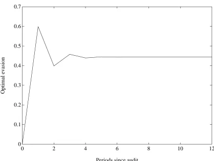
Figure 3 illustrates the dynamic behavior of a taxpayer after an audit. Again, the behavior is intuitively consistent with the model. Since audits are assumed to be successful at discovering all of a taxpayer’s undeclared income, a taxpayer in the first year after an audit has much less to lose from being audited again than would someone with an undiscovered recent history of past evasions. Consequently, there is an incentive for taxpayers to evade a significant amount in years following audits, in effect overshooting the conditional steady-state level of evasion.21 In the second year
18
We have also examined the implications of the functionπ(e) =peγ. Values ofγless than unity may generate eva-sion behavior that exhibits considerable instability at the individual level (since the evaeva-sion function is discontinuous at a point). Thus the assumption of convexity forπ in many of the propositions of this section is important.
19
The parameter values areα= 0.25,p= 0.75,β= 0.96, andr=g= 0.02. These are the parameter values used in the simulations depicted in Figures 2-7 unless explicitly stated otherwise.
20The proof of existence and uniqueness of such a point was sketched in footnote 14. 21
following an audit, taxpayers need to be conscious of their excessive evasion of the year before, and therefore reduce their evasion to a level below the conditional steady state. After a short span of dampening oscillation, this process converges to a steady state in which a taxpayer who is not audited evades the same fraction of income in consecutive years.
Changes in incomes and tax rates introduce differences between past evaded amounts and contemporaneous conditional steady state levels, thereby generating rich evasion dynamics. Unan-ticipated tax rate and income changes generate similar dynamics, since they effectively alter relative stocks of past evasions. To study how individuals react to changes in income and tax rates, the model described so far needs to be extended to incorporate these (and other) parameter changes. For simplicity, and without affecting the qualitative nature of the conclusions derived from the exercises that follow, we assume that individuals have static expectations about future parameters, so that, in periodt, individuals expect the growth rate ofτ y between periodstand t+ 1, denoted g≡ E[(τt+1yt+1−τtyt)/τtyt], to prevail into the indefinite future. They also believe that the current (periodt) audit function and interest rate will remain unchanged forever.
In the model described by (3), neither tax rates nor income levels directly affect evasion behavior. What does affect evasion is the magnitude of past evasion (et−1) normalized by differences between past and current income and tax rates (x). Hence, if the tax rate changes at timetin an unexpected, once-and-for-all manner, and income likewise grows in an unexpected, once-and-for-all manner, so that τ y increases by a fraction g− different from g (i.e., τ
tyt 6= (1 +g)τt−1yt−1), then the static expectations assumption implies that the optimal evasion level for period t can be obtained by evaluating the evasion function (corresponding to the values ofx and g expected to hold into the indefinite future) at
1 +g 1 +g−et−1
instead ofet−1.
drop of the year before, and consequently overshoots the steady-state evasion level on the high side. Oscillations ensue, quickly converging to the original steady state. Since the evasion function does not depend on the tax rate, and the expected growth rate of τ y is the same before and after the tax rate is lowered, the conditional steady state does not change. Symmetric dynamics characterize tax rate increases, and also characterize changes in the income growth rate.
Changes in enforcement intensity influence conditional steady-state evasion levels as well as short-term dynamics. Figure 5 depicts the effect of reducing enforcement intensity fromp= 1.0 to p= 0.75 for an unaudited individual who is in the conditional steady state prior to the enforcement change. The reduced enforcement intensity encourages additional evasion, particularly in the first year of the reform (period 12 in the figure), when not only is enforcement intensity reduced but the stock of prior unaudited evasion is smaller than the new conditional steady state.22 Evasion in the first year following the enforcement change overshoots the new conditional steady-state level; evasion in the second year falls below the new conditional steady state, and a process of convergence ensues. Greater enforcement intensity generates the same dynamics with opposite signs.
3
Aggregate Implications
Aggregate tax evasion behavior may differ from the individual behavior described in section 2.3, since individual situations differ and a certain fraction of the population is audited each year. The fraction audited is itself a function of the government’s enforcement intensity and individual behavior that responds to changes in enforcement intensity, income, and tax rates. Aggregate behavior is a weighted average of the behavior of individuals in different situations, with weights endogenously determined.
It is interesting to note that when the underlying parameters (enforcement, income growth, interest rate, and tax rate) do not change, the cross-section of evasion rates converges to a steady state (invariant distribution) and aggregate evasion approaches a limit. Once an economy with a
22
large number of taxpayers approaches the invariant distribution, the law of large numbers implies that aggregate evasion does not vary over time - even though individual evasion rates vary due to the fact that some individuals are audited while others are not. This steady state is distinct from an individual taxpayer’s conditional steady state described in section 2, since an individual’s steady state is conditional on not being audited, while the economy’s steady state is conditional on a distribution of individual audits across taxpayers with differing evasion histories.
Aggregate tax evasion behavior responds to aggregate shocks to underlying parameters in a manner that closely resembles the responses of unaudited individuals who start in the conditional steady state. In part, this feature of aggregate behavior reflects the rather small fraction of the population that is audited each year.
Figure 6 pictures the response of aggregate evasion to a 33 percent increase in the tax rate. As in figure 4, evasion responds by rising in the first period after the tax change, and falling below the steady-state level in the second period, before oscillating toward the original steady-state level. The path pictured in figure 6 uses the invariant distribution of taxpayers at original parameter values as the initial cross section of evasion rates. Since the invariant distributions both before and after the tax change are identical, the evasion rate converges ultimately to the value it took prior to the tax change. A tax rate reduction would generate a symmetric response pattern with opposite signs.
Figure 7 traces the aggregate impact of an increase in the enforcement intensity from p= 0.75 to p = 1.0. Again, the population of taxpayers prior to the enforcement change is assumed to be at its invariant distribution based on original parameter values, and, as with tax rate changes, aggregate responses resemble the behavior of individual taxpayers who have not been audited. This time, though, the new steady state level of evasion is lower than its pre-change value. Reduced enforcement intensity generates a similar, but oppositely-signed, pattern.23
23
4
Dynamic Patterns of U.S. Tax Evasion, 1947–1993
This section analyzes the pattern of aggregate U.S. tax evasion over the postwar period, paying particular attention to the dynamic issues discussed in sections 2 and 3.
4.1 Data
The fact that tax evasion is illegal makes it difficult for governments to obtain reliable estimates of its magnitude. There is no shortage of attempts to estimate the extent of tax evasion in the United States and elsewhere, but all face the difficulty that measures of evasion are inherently suspect. Another limitation is that continuous time series information on tax evasion is available only for country-level aggregates. In spite of these limitations, measured tax evasion rates exhibit certain empirical regularities, in particular a positive correlation with marginal tax rates and a negative correlation with enforcement intensities.24
One widely-used measure of evasion is based on the notion that personal income as calculated for national income accounting purposes (and properly adjusted for conceptual differences) should, in the absence of tax evasion, equal adjusted gross income reported on tax returns. The national income and product accounts calculate personal income based only in small part on income as reported in personal tax returns, so this measure of income is presumably very little affected by evasion propensities.25 The Bureau of Economic Analysis of the U.S. Department of Commerce reports this measure of the aggregate U.S. tax gap for every year since 1947.
Tax rate information is somewhat more problematic, since the relevant tax rate is the rate on marginal reported income. In a progressive income tax system, this rate is endogenous to the amount of income evaded and to the composition of the evading population. The tax rates used in the regressions are the statutory federal marginal rates that apply to taxpayers with family incomes equal to the mean income of the top quintile of the income distribution as reported by the Bureau
24
Feige (1989) and Cowell (1990, pp. 17-27) survey the available estimates of tax evasion in large samples of countries. The determinants of tax evasion behavior appear to be roughly consistent across available time series studies (Crane and Nourzad (1986) and Poterba (1987)) and cross-sectional studies (Clotfelter (1983), Slemrod (1985), Witte and Woodbury (1985), Dubin and Wilde (1988), and Feinstein (1991)), and conforms to tax collection patterns in the panel analyzed by Dubin et al. (1990). In the only available study of taxpayer behavior in consecutive years, Erard (1992) finds that taxpayers who are audited in one year are more likely than others to be caught evading in the subsequent year. Since audits are not randomly assigned, however, this finding may simply reflect that taxpayers have persistent characteristics.
of the Census. All of the regressions were re-run using the average federal tax rate, and using the marginal federal rate that applies to a family with the country’s mean income, with little change in the results. The marginal tax rate of families in the top quintile of the income distribution captures general movements in marginal tax rates, but is undoubtedly a noisy indicator of the marginal tax rates of typical evaders.
The enforcement variable is the fraction of individual income tax returns audited each year, as reported in the Annual Report of the Commissioner of Internal Revenue. This variable exhibits a widely-noted downward secular drift. Alternative possible enforcement indicators include real per capita enforcement expenditures and IRS employees as a fraction of the taxpaying population.26
All of these enforcement intensity indicators are limited by their inability to reflect changes in the real effectiveness of enforcement relative to individuals’ opportunities to hide their incomes. Changes in the cost of information processing have greatly increased the effectiveness of the IRS in certain dimensions, such as the ability to match the information in 1099 forms electronically to taxpayer returns. At the same time, individuals’ increased access to information processing lowers the cost of various tax evasion tactics. The net change in real enforcement may be best captured, if only imperfectly, by the audit rate.
4.2 Retrospective Enforcement
The model described in sections 2–3 is premised on the notion that taxpayers believe that if they are caught evading taxes this year they will be investigated by the IRS for prior years. While this specification is consistent with anecdotal evidence and warnings published in popular taxpayer guides, individual beliefs and individual experiences are likely to vary. Due to the extremely limited nature of the available information about tax audits, this specification cannot be tested directly. It is, however, possible to use aggregate data to identify the extent to which penalties imposed by IRS investigators reflect not only current but also past evasion.
The model implies that the amount of IRS-imposed fines and penalties subsequent to audits in the current year (denoted Γt) is a function of the penalty rateα, the probability of audit, and the
26See Hunter and Nelson (1996), who estimate a tax enforcement function for the United States based on observable
volume of current and past evasion:
Γt= (1 +α)πt(et)[etτtyt+ (1 +r)et−1τt−1yt−1+...+ (1 +r)net−nτt−nyt−n]upt (12)
in whichupt is the residual andndenotes the number of earlier years whose tax returns are subject to examination by the IRS upon finding that a taxpayer underreports income items on a current return. The specification in (12) leaves open the relevant size ofn.
Tax revenue from individual self-reports is denoted Rt and is given by:
Rt= (1−et)τtyturt (13)
in whichur
t is the residual of the revenue function. Dividing both sides of (12) by (13), and taking logs, yields normalized to account for accrued interest, subsequent income growth, and any tax rate changes between periodt−iand period t. The residual in (14) isut≡lnupt−lnurt.
The point of estimating (14) is to identify the effects of lagged evasion on current audit-imposed penalties. In doing so, it is useful to transform (14) in a way that offers linear tests of the inclusion of various lags ofe. The third term on the right side of (14) equals
ln et+ Taylor expansion a valid approximation to the value of the second term of (15),
ln
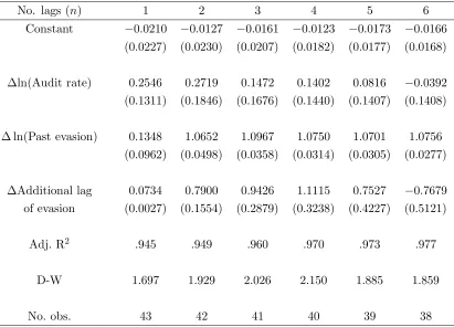
lies between 0.32 and 0.39, well below the unit value predicted by (14). Multiple lags of eappear to influence current audit-related penalties, as indicated for example in column 3 by the coefficient of 1.070 on the sum of current evasion plus two of its lags. The third lag of evasion appears to be appropriately included as well, since its estimated coefficient, 1.332, differs significantly from zero but not from the coefficient on current and two lags of evasion. The very low values of the Durbin-Watson statistics in these level specifications suggest, however, that first-differencing the sample is necessary in order to draw valid inferences.
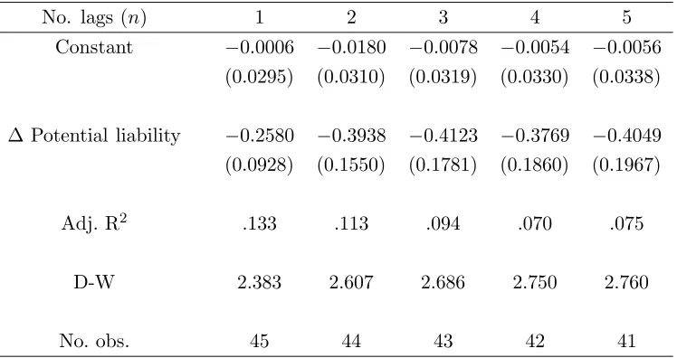
Table 2 presents estimates of first differences of (14). Here, too, multiple lags of e positively influence current fines and penalties. In the specification reported in column 3, current plus two lags ofehas an estimated coefficient of 1.0967, and the estimated coefficient onet−3 is 0.9426. The results reported in column 5 suggest that the sixth lag of e does not positively influence current fines and penalties. This result is consistent with estimates of an unrestricted distributed lag form of (14), reported as Appendix Table B4, in which the Schwarz statistic is maximized by the specification that includes current plus five lags ofe. The estimated coefficient on the audit rate is insignificant in all of the first difference specifications.
The finding that current-year penalties are functions of past evasion, the best fit being the sum of current evasion and five of its lags, offers three useful pieces of information. The first is that this pattern is consistent with retrospective auditing. The finding does not, in itself, constitute proof that auditing is retrospective, since an alternative possibility is that the IRS simply takes a very long time to determine which returns to audit and to complete the audits it selects. But evidence from popular accounts of IRS behavior suggests that, in fact, most audits take place soon after a return is filed, and almost always within one and a half years.27
A second implication of the penalty regressions is that the national income accounts-based measure of tax compliance is consistent with an independent indicator of compliance, which is reassuring given the difficulty of estimating tax evasion rates by any method. The third implication is that, since the three-year U.S. statute of limitations is extended to six years in cases of “major”
27
evasions,28 “major” evaders may account for the bulk of penalties imposed by the IRS.
4.3 Reduced Form Evasion Specifications
The model specified in section 2, and for which aggregate implications are depicted in section 3, is consistent with two alternative empirical specifications of the aggregate evasion process. In the reduced form specification of the model, aggregate evasion is a function of audit intensity as well as changes in income and tax rates. In the structural specification of the model, aggregate evasion is a function of lagged evasion (properly corrected for income and tax changes).
Reduced form specifications stem from the comparative static exercises analyzed in section 3, taking the initial distribution of evasion rates to be the invariant distribution. If the variation in et−1 is small relative to that in τt−1yt−1, then contemporaneous evasion becomes a function of current audit intensity and first differences in income and tax rates. The model implies that audit intensity should be negatively correlated with evasion rates, while income and tax changes should be positively correlated with evasion rates.
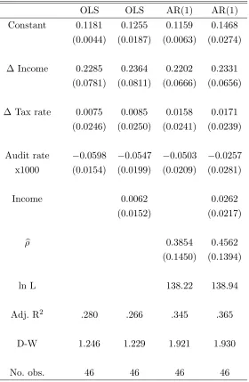
Table 3 presents estimates of the simple level specification of the reduced form of the model.29 The results are broadly consistent with the theory sketched in sections 2–3. In the regression reported in the first column, 10% income growth is associated with 2.3% greater tax evasion. The estimates also imply that 1% higher audit rates reduce evasion by 0.6%, and that 1% higher tax rates increase evasion by 0.8%, though the latter effect is not statistically significant. The regression reported in column 2 adds log income as an explanatory variable; its estimated coefficient is insignificant, and its inclusion affects the other estimated coefficients very little.30 The Durbin-Watson statistics associated with the level specifications of the reduced form model suggest that it may be appropriate to correct for autocorrelation. Columns 3–4 describe regressions that add estimated AR(1) corrections with results that are very similar to those presented in columns 1–2.
One of the difficulties that arise in interpreting the regressions reported in Table 3 is the po-tential role of measurement error in biasing the estimated coefficients. Since personal income is probably measured with error, and tax evasion rates are constructed from differences between in-come reported on tax forms and personal inin-come measured for national accounting purposes, it is
28
“Major” tax evasions occur when taxpayers underreport income by more than 25% of the total.
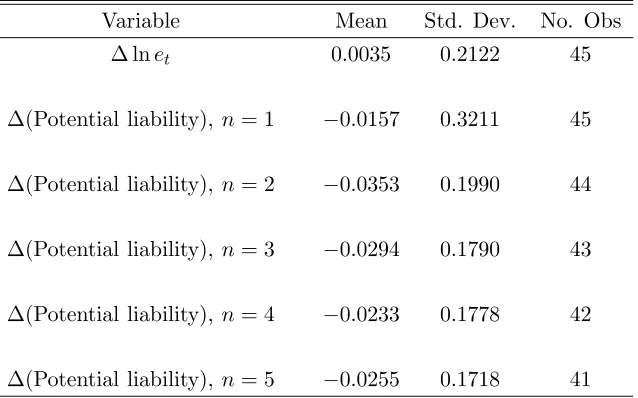
29Appendix B provides means and standard deviations of regression variables. 30
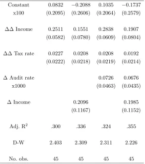
possible that noise in the income variable generates a spurious correlation between evasion rates and income growth. Weighing against this possibility is the usual effect of measurement error in bi-asing downward the estimated coefficients. The net impact of measurement error on the estimated coefficients depends, therefore, on the relative magnitudes of these two effects. Appendix D offers calculations indicating that, unless measurement error in the growth rate of income is one order of magnitude larger than common sense indicates is possible, the reduced form results are robust to measurement error — and indeed, may well understate the true effect of income growth on evasion. The reduced form specification of the model can be estimated in first differences as well as levels. Table 4 reports estimated coefficients from first difference specifications. The results are generally consistent with those reported in Table 3, the major difference being the insignificance (and positive sign) of coefficients on first differences of enforcement intensities. Since audit rates are no better than passable proxies for enforcement intensities, it is not surprising that first differences of this variable have little measurable impact on taxpayer behavior.31 Columns 1–2 of Table 4 report first difference specifications that omit audit rates, while columns 3–4 report first difference specifications that include audit rates. The estimated coefficient on the second difference of income in column 1 implies that 10% income growth is associated with 2.5% greater tax evasion, which is similar to the effect estimated in levels. Tax rate changes have positive but insignificant effects on evasion, as is true in the level specifications as well.
It is possible to impose additional structure on the reduced form specification of the model by including time-varying determinants of et−1, of which obvious candidates include lagged changes in income and tax rates.32 The oscillations pictured in figures 4 and 5 reflect the impact of these determinants of subsequent evasion.
If enforcement intensity follows a random walk, then enforcement proxies (such as audit rates) can be omitted from the right side of first-difference evasion specifications, since changes in enforce-ment have the same properties as the residual. Table 5 presents estimated coefficients from first difference reduced form specifications that omit audit intensity but add lagged second differences of income and tax rates. As in the regressions reported in Table 4, the coefficients on the second
31
Another possibility is that taxpayers learn very slowly about changes in enforcement levels, as Erard (1992) suggests.
32Lagged tax enforcement intensity has an ambiguous effect on contemporaneous tax evasion. Stronger past
difference of tax rates are positive and insignificant; the coefficients on the lagged second difference of tax rates equal zero. But the estimated coefficients on income changes have the predicted signs: second differences of income have positive effects on evasion while lagged second differences have negative effects. The estimates reported in column 2 imply that 10% income growth is associated with 5.7% more tax evasion contemporaneously but 1.7% less tax evasion in the subsequent year.
The reduced form regressions offer evidence that is consistent with the model described in sections 2–3. The estimates indicate that exogenous variables (such as lagged income and tax rates) that are positively associated with past undetected evasion are also negatively correlated with contemporaneous tax evasion. The next section considers estimating equations in which lagged evasion enters directly.
4.4 Structural Estimation
This section presents estimates of an approximation to the first order condition associated with the taxpayer’s optimization problem (3) when taxpayers have static expectations concerning future economic variables.
The first order condition associated with (6) is:33
1
whereetdenotes the taxpayer’s optimal evasion rate assuming that this period’s growth rate ofτ y will prevail into the future.34
Take the audit function to be of the form:
πt(e) =pteγ, (18)
withγ >1 to ensure both a continuous policy function (see Proposition 2.5) and an interior solution (see Appendix F). To derive the estimating equation, use Proposition 2.6 to approximate [W(et)− W(0)] in (17) by etW′(et), and use (10) to substitute for the latter. After some straightforward
33
Appendix F identifies sufficient conditions for this problem to have an interior solution.
34
algebra this leads to
Since the sample mean of the audit rate πt(et) is 0.026, the denominator of the term on the right-hand side of (19) is safely approximated by unity. Substitutingpteγforπt(et) in the numerator of the term on the right side implies:
e−t(γ−1) ≃ (1 +α)γxtptet−1. (20)
Consider the case in which logptfollows a random walk with driftµ, so that logpt= logpt−1+µ+εt, in which εt is a white noise residual. Taking the derivative of the logarithms of both sides of the above equation then implies:
The above derivation can be extended to the case in which the IRS audits more than one period of past returns, leading to
Table 6 presents estimates of differing specifications of this linear approximation to the structural evasion equation. Column 1 reports results of a specification in which only current and one lag of et are included on the right side of the estimating equation. The coefficient of−0.25 on lagged evasion is significantly different from zero, and implies a value of γ equal to 4.9. Columns 2–5 report results from specifications that sequentially include additional lags ofet, in all of which the coefficient on lagged evasion is approximately 0.4 and therefore implies that γ equals 3.5.
The implications of the structural estimates are quite consistent with those of the reduced form estimates. Aggregate evasion rates are higher in years in which the stock of past evasion,
considers the implications of these findings.
5
Implications
The behavior of American taxpayers carries implications for the likely effects of various tax en-forcement policies. This section considers three issues in particular: the effect of retrospective auditing, the effect of penalties for noncompliance, and the effect of tax amnesties. The regressions presented in section 4 estimate structural aspects of tax compliance in the United States on the basis of taxpayer reactions to short-term shocks to income and other variables; it is then possible to use these behavioral parameters to draw inferences about the way in which enforcement policies influence long-run as well as short-run tax compliance behavior.
5.1 The Deterrent Effect of Retrospective Audits
The fact that tax authorities are entitled to examine a taxpayer’s returns for previous years, and impose penalties for deficiencies, has an understandably chilling effect on evasion behavior, since the cost of triggering an audit this year includes penalties for evasion in earlier years. An alternative legal regime, and the one typically considered in the tax evasion literature, is a system in which the government audits only the current tax return, so any past evasions remain undetected and unpunished. It is possible to use the parameters obtained in section 4 to estimate the extent to which removing the threat of retrospective audits would stimulate additional tax evasion.
Equation (2) describes the behavior of taxpayers who select their evasion levels without con-cern for retrospective audits. Applying the enforcement function (18) to (2), the representative individual’s first-order condition becomes:
est =
1
(1 +α) (1 +γ)pt
1/γ , (23)
in whichest denotes the evasion level chosen by a taxpayer who behaves according to a static rule that omits consideration of retrospective audits.
Current values of pt can be inferred from observed audit and evasion behavior by inverting the enforcement function (18):
pt=eπtee−tγ (24)
in which πe denotes the observed probability of audit in period t, and eet is the observed evasion level. At current enforcement levels given byγ and pt, (23) and (24) together imply:
est/eet= [(1 +α) (1 +γ)eπt]−1/γ (25)
which indicates the extent to which evasion would differ from its observed level if taxpayers were unconcerned about being caught for their past evasions.
The value of α is fixed by law at 0.25, and regressions presented in section 4 imply a γ value roughly equal to 3.5. Observed audit rates, πet, change over time, taking a mean value of 0.0263 in the sample. Evaluating πet at this mean, and taking 0.25 for α and 3.5 for γ, the term on the right side of (25) equals 1.72. This figure, if taken literally, implies that evasion would increase by 72% if Americans became unconcerned about retrospective audits (or equivalently that evasion is currently 42% below its level without retrospective audits). Evaluating the right side of (25) separately for each year generates a series with a mean value of 1.83, similarly implying that tax evasion would be 83% higher in the absence of retrospective enforcement. By either calculation, es t
significantly exceeds eet.
The exercise that generates the 72% figure is one in which taxpayers lose their fear of retrospec-tive audits while the key tax enforcement parameters —γ andpt— do not change. The parameter γ expresses the efficiency of the process by which the IRS identifies which tax returns to audit, since higher values of γ correspond to individual audit probabilities that increase more rapidly as the fraction of income evaded increases. In the empirical work presented in section 4, γ is taken to be constant over time — an assumption for which there are no attractive alternatives, since changes in γ cannot be directly measured. Holding γ constant as the retrospective nature of the enforcement regime changes is, in this context, quite reasonable, since information from past tax returns is not used to identify which returns to audit this year.
function (18) implies a higher number of audits. With a fixed enforcement budget, it is possible that the IRS would be unable to accomodate this greater demand for audits, in which case pt would have to fall and the level of tax evasion rise still further. In this sense, the 72% figure may represent a lower bound on the extent to which evasion might rise in reaction to a nonretrospective enforcement regime.36
A 72% difference in the rate of tax evasion is not at all trivial, so it is worth considering why concern on the part of taxpayers that they will face retrospective audits can have such a major effect on behavior. In the context of the model, tax evasion is limited by the tradeoff that consumers face between the benefits of reducing taxes today by increasing their evasion and two costs associated with greater evasion: the cost of increasing today’s audit probability plus the cost of higher penalties for today’s evasion if subject to an audit in the future. Given the rather low audit probabilities that taxpayers face, the cost associated with triggering a current audit is considerably larger than the expectation of future penalties for current evasion. Audits are roughly one-sixth as costly if they trigger penalties only for current evasion and not for five earlier years of tax evasion. Predicted evasion does not increase to six times its prior value, however, due to the convex shape of the audit function. Instead, evasion increases to approximately 61γ = 6
1
3.5 = 1.67 times the value it
takes if taxpayers are concerned about audits for earlier years. Given the size of the additional potential tax liability associated with retrospective auditing, then, 72% is a reasonable estimate of the additional evasion associated with its removal.
5.2 Penalties for Noncompliance
An American who is caught evading taxes is generally required to pay a penalty equal to 25% of unpaid taxes in addition to repaying the taxes he owes. The modest size of this penalty rate is widely believed to encourage tax evasion and thereby to be responsible for the current rate of evasion in the United States. It is possible to use the estimated value of γ reported in section 4 to evaluate the effect of penalties for noncompliance on current evasion levels. The results suggest that, while higher penalties discourage evasion, dramatically higher penalty rates would be required
36Another possibility is that the IRS would be able to reallocate resources previously used to investigate past tax
in order to have a large impact on tax evasion rates.
Consider the linearized version of the tax evasion model analyzed in section 4. Differentiating both sides of (20) with respect toα and rearranging terms produces:
η≡ det dα
α et
= − α
(γ−1) (1 +α) (26)
in whichη is the elasticity of evasion with respect to the penalty rate. Substituting α= 0.25 and γ = 3.5 into (26) generates an implied value of η =−0.08. This estimate indicates that doubling the penalty rate reduces tax evasion by just 8% of its current level. This small behavioral response reflects two aspects of tax penalties: the low rate at which penalties are currently applied, and the fact that tax enforcement relies rather little on penalties.
In order to illustrate the impact of tax penalties, consider a scenario in which the government abolishes penalties for tax evasion, so the only cost of being caught in a tax audit is the obligation associated with current and past unpaid taxes. Even in the absence of penalties, taxpayers generally have incentives to report to the IRS large fractions of their incomes, since excessive evasion makes an audit extremely likely and therefore defeats the purpose of evasion. The more elastic is the audit function (corresponding to higher values of γ), the greater the extent to which taxpayers reduce their evasion in order to avoid being audited and caught. For those situations in which governments impose penalties for evasion, higher values of γ reduce the magnitude of η, as indicated by (26). For the United States, the estimated value of γ = 3.5 implies that penalties play a rather small role in deterring tax evasion.
5.3 Tax Amnesties
A typical tax amnesty is one in which a government gives its residents the opportunity to declare any previously-unreported income to tax authorities. Taxpayers participating in amnesties must pay their back taxes, but are not subject to penalties. Tax amnesties are popular among American states, and appear to generate small but nonzero tax revenue in the short run — though there is a lively debate about why it is that taxpayers who once elected not to report their incomes to the government subsequently change their minds and participate in amnesties.37 One common criticism
of amnesty initiatives is that they may depress tax collections in the long run. The argument is based on the notion that a government granting its first amnesty creates the perception that it may offer additional amnesties in the future. If the prospect of a future amnesty encourages current tax evasion, then even one-time amnesties may reduce tax revenues in the steady state.
The model described in section 2 suggests an entirely different, and short-run, effect of tax amnesties on tax collections. An individual electing to participate in an amnesty eliminates his stock of accumulated past evasion and therefore has the least to lose of anyone in the population if audited the following year. Such individuals have strong incentives to evade in the years following amnesties, their optimal evasion patterns mimicking the behavior of taxpayers who have just been audited (depicted in figure 3). Aggregate tax revenue is therefore likely to fall in years after amnesties, though tax collections in the steady state are unaffected by this dynamic consideration.
6
Conclusion
The ability of tax authorities to investigate returns for earlier years makes rational taxpayers who have something to hide reluctant to draw attention to their current tax returns by evading excessively. Retrospective auditing therefore creates incentives that generate short-run tax evasion cycles in response to shocks. For habitual evaders, tax rate changes and income fluctuations can initiate such cycles, since current evasion is a function of the stock of undiscovered past evasion normalized by current tax rates and current income. It follows that short-run aggregate tax evasion is a function of aggregate changes in tax rates and income.
Evidence for the United States is consistent both with retrospective auditing behavior by the IRS and with rational responses by individual taxpayers to the prospect of retrospective audits. Three empirical regularities appear in aggregate data. The first is that annual penalties imposed by the IRS subsequent to audit are functions of contemporaneous tax evasion plus up to five of its lags. The second is that the tax evasion rate is positively correlated with income growth and tax rate changes. And the third is that current evasion is negatively related to several lags of past evasion normalized for income and tax changes.
by 72% — from 10.6% of current income to 18.2% — in the absence of retrospective auditing. The ability of the IRS to identify the most promising returns to audit is a far more powerful enforcement tool than is a high penalty on evaded income, since doubling the penalty rate from 25% to 50% would reduce evasion rates by only 8%, from 10.6% to 9.7%. And tax amnesties that generate higher tax collections immediately may significantly reduce tax collections in subsequent years, when taxpayers have less to fear from retrospective audits.
Appendices
A
Data Sources
The income variable used in the empirical work is individual adjusted gross income (AGI) as cal-culated from the U.S. national income and product accounts and reported by the Internal Revenue Service on a calendar year basis for 1947-1993. Reported income (Rt) is AGI as reported on individ-ual tax returns. Conceptindivid-ually, income as measured by the national income and product accounts and reported income should be equal in the absence of tax evasion. Both variables are converted to per capita terms by dividing by the number of individual tax filers. Data on AGI as calculated from the national income and product accounts, AGI as reported on individual tax returns, and numbers of tax filers are reported in Internal Revenue Service (1995a, p. 201). Nominal variables are adjusted for inflation using the personal consumption deflator from the U.S. national income and product accounts.
Tax rates are marginal federal income tax rates for married taxpayers (filing jointly) with incomes equal to the mean family income of the top quintile of the U.S. income distribution as reported by the U.S. Census (various issues). Marginal federal tax rates are reported by the Tax Foundation (various issues).
The number of tax audits is reported annually for 1947-1992 by the Annual Report of the Commissioner of Internal Revenue (various issues), and, for 1993-1994, in Internal Revenue Service (1995b). These sources report figures on a fiscal year basis, and are not perfectly consistent over time, so it is necessary to perform some adjustments in order to make them correspond properly to calendar year data on tax evasion, income, and tax rates. Since 1976, U.S. government fiscal years start on October 1 of the previous calendar year and continue to the following September 30. (Prior to 1976, fiscal years started on July 1 and continued to the following June 30.) Tax audits are attributed to the preceding calendar years, so that, for example, audits performed in fiscal year 1982 (October 1, 1981 to September 30, 1982) are assumed to apply to tax returns for calendar year 1981 for purposes of calculating audit rates.
fraction of 1951 audits that represent audits of corporate tax returns (5.18%). The definition of an “audit” changed during 1953 and part of 1954, since “audits” during 1947-1952 include mathematical corrections and verifications that are excluded from the definition of an “audit” after 1953. The 1955 Annual Report of the IRS Commissioner estimates that 127,000 “audits” reported for 1954 were actually mathematical corrections and verifications, so reported “audits” for 1954 are reduced by this number in calculating audit rates. The 1955 Report indicates that, in 1954, true audits represented 50.97% of what would have been audits as previously defined (audits plus mathematical corrections and verifications). Consequently, reported audits for 1947-1952 are multiplied by 0.5097 in calculating audit rates. Since 1953 was a transition year for audit definitions, reported audits for 1953 receive half of the 1947-1952 adjustment (they are multiplied by 0.7548) in calculating the audit rate for that year. The definition of an “audit” again changed in 1993. IRS (1995b) reports audits for 1992, using the new definition of an “audit;” by comparing this 1992 figure with the figure reported in the 1993 Annual Report (and calculated under the previous definition of an “audit”), it follows that, in 1992, “audits” as defined pre-1993 were 86.30% of “audits” as defined starting in 1993. Consequently, audit rates for 1993 and 1994 are multiplied by 86.30% to make them comparable to pre-1993 rates.
Penalties and fines imposed subsequent to audits of individual tax returns are reported annually for 1947-1992 by the Annual Report of the Commissioner of Internal Revenue (various issues), and, for 1993-1994, in IRS (1995b). As with audit statistics, these figures are reported on a fiscal year basis, and are not perfectly consistent over time, so it is necessary to perform some adjustments in order to make them correspond properly to calendar year data. Penalties and fines are attributed to the second preceding calendar year, so that, for example, penalties and fines assessed in fiscal year 1985 (October 1, 1984 to September 30, 1985) are assumed to apply to tax returns for calendar year 1983.


![Keterkaitan Antara Musim Terhadap Produksi Susu Sapi Perah Fries Holland [studi kasus : PT. Naksastra kejora, Temanggung, Jawa Tengah]](data:image/gif;base64,R0lGODlhAQABAIAAAP///wAAACH5BAEAAAAALAAAAAABAAEAAAICRAEAOw==)