Turin Lectures
F. Dalbono - C. Rebelo
∗POINCAR ´
E-BIRKHOFF FIXED POINT THEOREM AND
PERIODIC SOLUTIONS OF ASYMPTOTICALLY LINEAR
PLANAR HAMILTONIAN SYSTEMS
Abstract. This work, which has a self contained expository character, is devoted to the Poincar´e-Birkhoff (PB) theorem and to its applications to the search of periodic solutions of nonautonomous periodic planar Hamil-tonian systems. After some historical remarks, we recall the classical proof of the PB theorem as exposed by Brown and Neumann. Then, a variant of the PB theorem is considered, which enables, together with the classical version, to obtain multiplicity results for asymptotically linear planar hamiltonian systems in terms of the gap between the Maslov in-dices of the linearizations at zero and at infinity.
1. The Poincar´e-Birkhoff theorem in the literature
In his paper [28], Poincar´e conjectured, and proved in some special cases, that an area-preserving homeomorphism from an annulus onto itself admits (at least) two fixed points when some “twist” condition is satisfied. Roughly speaking, the twist condition consists in rotating the two boundary circles in opposite angular directions. This con-cept will be made precise in what follows.
Subsequently, in 1913, Birkhoff [4] published a complete proof of the existence of at least one fixed point but he made a mistake in deducing the existence of a second one from a remark of Poincar´e in [28]. Such a remark guarantees that the sum of the indices of fixed points is zero. In particular, it implies the existence of a second fixed point in the case that the first one has a nonzero index.
In 1925 Birkhoff not only corrected his error, but he also weakened the hypothesis about the invariance of the annulus under the homeomorphism T . In fact Birkhoff him-self already searched a version of the theorem more convenient for the applications. He also generalized the area-preserving condition.
Before going on with the history of the theorem we give a precise statement of the classical version of Poincar´e-Birkhoff fixed point theorem and make some remarks. In the following we denote byAthe annulusA:= {(x,y)∈ R2 : r12 ≤ x2+y2 ≤ r22,0<r1<r2}and by C1and C2its inner and outer boundaries, respectively.
∗The second author wishes to thank Professor Anna Capietto and the University of Turin for the
invita-tion and the kind hospitality during the Third Turin Fortnight on Nonlinear Analysis.
Moreover we consider the covering space H := R×R+0 ofR2\ {(0,0)}and the
projection associated to the polar coordinate system5 : H −→R2\ {(0,0)}defined
by5(ϑ,r)=(r cosϑ,r senϑ). Given a continuous mapϕ : D⊂R2\ {(0,0)} −→
R2\ {(0,0)}, a mapeϕ : 5−1(D)−→H is called a lifting ofϕto H if
5◦eϕ = ϕ◦5.
Furthermore for each set D⊂R2\ {(0,0)}we setD :˜ =5−1(D).
THEOREM1 (POINCARE´-BIRKHOFFTHEOREM). Letψ : A−→Abe an area-preserving homeomorphism such that both boundary circles ofAare invariant under ψ (i.e.ψ(C1)=C1andψ(C2)=C2). Suppose thatψadmits a liftingψeto the polar coordinate covering space given by
(1) eψ (ϑ,r) = (ϑ +g(ϑ,r), f(ϑ,r)),
where g and f are 2π−periodic in the first variable. If the twist condition
(2) g(ϑ,r1) g(ϑ,r2) < 0 ∀ϑ ∈R [twist condition] holds, thenψadmits at least two fixed points in the interior ofA.
The proof of Theorem 1 guarantees the existence of two fixed points (called F1
and F2) of eψsuch that F1−F2 6= k(2π,0), for any k ∈ Z. This fact will be very
useful in the applications of the theorem to prove the multiplicity of periodic solutions of differential equations. Of course the images of F1, F2under the projection5are
two different fixed points ofψ.
We make now some remarks on the assumptions of the theorem.
REMARK 1. We point out that it is essential to assume that the homeomorphism is area-preserving. Indeed, let us consider an homeomorphismψ : A −→Awhich admits the liftingψ (ϑ,e r)=(ϑ+α(r), β(r)), whereαandβare continuous functions verifying 2π > α(r1) > 0 > α(r2) > −2π,β(ri)= ri for i ∈ {1,2},β is strictly increasing andβ(r) > r for every r ∈ (r1,r2). This homeomorphism, which does not preserve the area, satisfies the twist condition, but it has no fixed points. Also its projection has no fixed points.
REMARK2. The homeomorphismψpreserves the standard area measure dx dy in R2and hence its liftψepreserves the measure r dr dϑ. We remark that it is possible to consider a lift in the Poincar´e-Birkhoff theorem which preserves dr dϑinstead of r dr dϑ
and still satisfies the twist condition. In fact, let us consider the homeomorphism T of R×[r1,r2] onto itself defined by T(ϑ,r) = (ϑ,a r2+b), where a= 1
r1+r2
and
b= r1r2
ofψe∗and fixed points T−1(F)ofψe. Finally, it is easy to verify thatψe∗is the lifting of an homeomorphismψ∗which satisfies all the assumptions of Theorem 1. This remark implies that Theorem 1 is equivalent to Theorem 7 in Section 2.
It is interesting to observe that if slightly stronger assumptions are required in The-orem 1, then its proof is quite simple (cf. [25]). Indeed, we have the following propo-sition.
PROPOSITION1. Suppose that all the assumptions of Theorem 1 are satisfied and
that
(3) g(ϑ,·)is strictly decreasing(or strictly increasing)for eachϑ. Then,ψadmits at least two fixed points in the interior ofA.
Proof. According to (2) and (3), it follows that for everyϑ ∈ Rthere exists a unique
r(ϑ)∈ (r1,r2)such that g(ϑ,r(ϑ))=0. By the periodicity of g in the first variable,
we have that g(ϑ +2kπ,r(ϑ)) = g(ϑ,r(ϑ)) = 0 for every k ∈ Z andϑ ∈ R. Hence as g(ϑ+2kπ,r(ϑ+2kπ ))=0, we deduce from the uniqueness of r(ϑ)that
r : ϑ 7−→r(ϑ)is a 2π−periodic function. Moreover, we claim that it is continuous too. Indeed, by contradiction, let us assume that there existϑ ∈Rand a sequenceϑn converging toϑwhich admits a subsequenceϑnksatisfying lim
k→+∞r(ϑnk)=b6=r(ϑ). Passing to the limit, from the equality g(ϑnk,r(ϑnk)) = 0, we immediately obtain
g(ϑ,b)=0=g(ϑ,r(ϑ)), which contradicts b6=r(ϑ).
By construction,ψ (ϑ,e r(ϑ)) = (ϑ +g(ϑ,r(ϑ)) , f(ϑ,r(ϑ)) ) = (ϑ , f(ϑ,r(ϑ)) ). Hence, each point of the continuous closed curveŴ⊂Adefined by
Ŵ= {(x,y)∈R2 : x=r(ϑ)cosϑ , y=r(ϑ)senϑ , ϑ∈R}
is “radially” mapped into another one under the operatorψ. Beingψarea-preserving and recalling the invariance of the boundary circles C1, C2 ofA under ψ, we can
deduce that the region bounded by the curves C1andŴencloses the same area as the
region bounded by the curves C1andψ(Ŵ). Therefore, there exist at least two points
of intersection betweenŴandψ(Ŵ). In fact as the two regions mentioned above have the same measure, we can write
Z 2π
0
Z r(ϑ )
r1
r dr dϑ = Z 2π
0
Z f(ϑ,r(ϑ ))
r1
r dr dϑ ,
which implies
Z 2π
0
r2(ϑ)− f2(ϑ,r(ϑ))
Morris [26] applied this version of the theorem to prove the existence of infinitely many 2π−periodic solutions for
x′′ + 2x3 = e(t),
where e is continuous, 2π−periodic and it satisfies
Z 2π
0
e(t)dt = 0.
If we assume monotonicity ofϑ+g(ϑ,r)inϑ, for each r , then also in this case the existence of at least one fixed point easily follows (cf. [25]).
PROPOSITION2. Assume that all the hypotheses of Theorem 1 hold. Moreover,
suppose that
(4) ϑ + g(ϑ,r)is strictly increasing(or strictly decreasing)inϑfor each r. Then, the existence of at least one fixed point follows, whenψis differentiable.
Proof. Let us suppose thatϑ 7−→ ϑ +g(ϑ,r)is strictly increasing for every r ∈ [r1,r2]. Thus, since
∂ (ϑ+g(ϑ,r))
∂ ϑ > 0 for every r , it follows that the equation ϑ∗=ϑ+g(ϑ,r)defines implicitlyϑas a function ofϑ∗and r . Moreover, taking into account the 2π−periodicity of g in the first variable, it turns out thatϑ = ϑ(ϑ∗,r)
satisfiesϑ(ϑ∗+2π,r) =ϑ(ϑ∗,r)+2π for everyϑ∗and r . We set r∗ = f(ϑ,r). Combining the area-preserving condition and the invariance of the boundary circles underψ, then the existence of a generating function W(ϑ∗,r)such that
(5)
ϑ = ∂W
∂r (ϑ
∗,r)
r∗ = ∂W ∂ϑ∗(ϑ∗,r)
is guaranteed by the Poincar´e Lemma.
Now we consider the functionw(ϑ∗,r)=W(ϑ∗,r)−ϑ∗r . Since, according to (5),
the following equalities hold
∂ w
∂ϑ∗ = r
∗ −r
∂ w
∂r = ϑ −ϑ
∗,
the critical points ofwgive rise to fixed points ofψ.
It is easy to verify thatwhas period 2π inϑ∗. Indeed, according to the hypothesis of boundary invariance and to (5), we get
W(ϑ∗+2π,r1) −W(ϑ∗,r1) =
Z ϑ∗+2π
ϑ∗
r∗(s,r1)ds =
Z ϑ∗+2π
ϑ∗
Furthermore, combining (5) with the equalityϑ(ϑ∗+2π,r) = ϑ(ϑ∗,r)+2π, we deduce
W(ϑ∗+2π,r)− W(ϑ∗+2π,r1) = Z r
r1
ϑ(ϑ∗+2π,s)ds
= Z r
r1
ϑ(ϑ∗,s)ds + 2π(r−r1)
=W(ϑ∗,r) − W(ϑ∗,r1) +2π(r−r1).
Finally, we infer that
w(ϑ∗+2π,r)−w(ϑ∗,r) =W(ϑ∗+2π,r)−W(ϑ∗,r)−2πr =W(ϑ∗+2π,r1)−W(ϑ∗,r1)−2πr1=0,
and the periodicity ofwin the first variable follows. Consider now the external normal derivatives ofw
(6) ∂ w
∂n f
C1
=(r∗−r, ϑ−ϑ∗)·(0,−1)=ϑ∗−ϑ,
(7) ∂ w
∂n f
C2
= (r∗−r, ϑ−ϑ∗)·(0,1) = ϑ−ϑ∗.
The twist condition (2) implies thatϑ∗−ϑ has opposite signs on the two boundary circles. Hence, by (6) and (7), the two external normal derivatives infC1andfC2have
the same sign. Beingwa 2π−periodic function inϑ∗, critical point theory guarantees the existence of a maximum or a minimum ofwin the interior of the covering space
e
A. Such a point is the required critical point ofw.
It is interesting to notice that as a consequence of the periodicity of g and f inϑ, the existence of a second fixed point (a saddle) follows from critical point theory.
As we previously said, in order to apply the twist fixed point theorem to prove the existence of periodic solutions to planar Hamiltonian systems, Birkhoff tried to replace the invariance of the annulus by a weaker assumption. Indeed, he was able to require that only the inner boundary is invariant under T . He also generalized the area-preserving condition. More precisely, in his article [5] the homeomorphism T is defined on a region R bounded by a circle C and a closed curveŴsurrounding C. Such an homeomorphism takes values on a region R1bounded by C and by a closed curve Ŵ1surrounding C. Under these hypotheses, Birkhoff proved the following theorem
THEOREM 2. Let T : R −→ R1be an homeomorphism such that T(C) = C and T(Ŵ)=Ŵ1, withŴandŴ1star-shaped around the origin. If T satisfies the twist condition, then either
or
•there is a ring in R(or R1)around C which is carried into part of itself by T (or T−1).
Since Birkhoff’s proof was not accepted by many mathematicians, Brown and Neu-mann [6] decided to publish a detailed and convincing proof (based on the Birkhoff’s one) of Theorem 1. In the same year, Neumann in [27] studied generalizations of such a theorem. For completeness, we will recall the proof given in [6] and also the details of a remark stated in [27] in the next section.
After Birkhoff’s contribution, many authors tried to generalize the hypothesis of invariance of the annulus, in view of studying the existence of periodic solutions for problems of the form
x′′ + f(t,x) = 0,
with f : R2−→Rcontinuous and T -periodic in t.
In this sense we must emphasize the importance of the works by Jacobowitz and W-Y Ding. In his article [22] Jacobowitz (see also [23]), gave a version of the twist fixed point theorem in which the area-preserving twist homeomorphism is defined on an annulus whose internal boundary (roughly speaking) degenerates into a point, while the external one is a simple curve around it. More precisely, he first considered two simple curvesŴi =(ϑi(·),ri(·)), i =1,2, defined in [0,1], with values in the(ϑ,r) half-plane r > 0, such that ϑi(0) = −π, ϑi(1) = π, ϑi(s) ∈ (−π, π ) for each
s ∈ (0,1)and ri(0) = ri(1). Then, he considered the corresponding 2π-periodic extensions, which he called againŴi. Denoting by Ai the regions bounded by the curveŴi (included) and the axis r = 0 (excluded), Jacobowitz proved the following theorem
THEOREM3. Letψ : A1−→ A2be an area-preserving homeomorphism, defined by
ψ(ϑ,r) = (ϑ +g(ϑ,r),f(ϑ,r)),
where
• g and f are 2π−periodic in the first variable; • g(ϑ,r) < 0 onŴ1;
• lim inf
r→0 g(ϑ,r) > 0.
Then,ψadmits at least two fixed points, which do not differ from a multiple of(2π,0).
Unfortunately the proof given by Jacobowitz is not very easy to follow. Subse-quently, using the result by Jacobowitz, W-Y Ding in [15] and [16] treated the case in which also the inner boundary can vary under the area-preserving homeomorphism. He considered an annular regionAwhose inner boundary C1and the outer one C2are
two closed simple curves. By Di he denoted the open region bounded by Ci, i=1,2. Using the result by Jacobowitz, he proved the following theorem
home-omorphism. Suppose that
(a) C1is star-shaped about the origin;
(b) T admits a liftingT onto the polar coordinate covering space, defined bye e
T(ϑ,r) = (ϑ + g(ϑ,r),f(ϑ,r)),
where f and g are 2π−periodic in the first variable, g(ϑ,r) >0 on the lifting
of C1and g(ϑ,r) <0 on the lifting of C2;
(c) there exists an area-preserving homeomorphism T0 : D2 −→R2, which satis-fies T0|A=T and(0,0)∈T0(D1).
Then,T has at least two fixed points such that their images under the usual coveringe projection5are two different fixed points of T .
We point out that condition (c) cannot be removed. Indeed, we can define A := {(x,y) : 2−2 < x2
+y2 < 22}and consider an homeomorphism T : A −→ R2 \ {(0,0)}whose lifting is given by eT(ϑ,r) =
ϑ+1−r,√r2+1. It easily follows thatT preserves the measure r dr dϑe and,
con-sequently, T preserves the measure dx dy. Moreover, the twist condition is satisfied, being g(ϑ,r)= 1−r positive on r = 1
2 and negative on r = 2. We also note that it is not possible to extend the homeomorphism into the interior of the circle of ra-dius 1/2 as an area-preserving homeomorphism, and hence (c) is not satisfied. Since
f(ϑ,r)= √r2+1 >r for every r ∈
1 2,2
, we can conclude that eT has no fixed
points.
In [29], Rebelo obtained a proof for Jacobowitz and Ding versions of the Poincar´e-Birkhoff theorem directly from Theorem 7.
The W-Y Ding version of the theorem seems the most useful in terms of the applica-tions. In 1998, Franks [18] proved a quite similar result using another approach. In fact he considered an homeomorphism f from the open annulusA=S1×(0,1)into
itself. He replaced the area-preserving condition with the weaker condition that every point ofAis non-wandering under f . We recall that a point x is non-wandering under
f if for every neighbourhood U of x there is an n>0 such that fn(U)∩U 6= ∅. Being ef , from the covering spaceAe= R×(0,1)onto itself, a lift of f , it is said that there is a positively returning disk for ef if there is an open disk U ⊂ eA such that ef(U)∩U = ∅and efn(U)∩(U+k)6= ∅for some n,k >0. A negatively return-ing disk is defined similarly, but with k < 0. We recall that by U +k it is denoted
On the lines of Birkhoff [5], some mathematicians generalized the Poincar´e-Birkhoff theorem, replacing the area-preserving requirement by a more general topo-logical condition. Among others, we quote Carter [8], who, as Birkhoff, considered an homeomorphism g defined on an annulusAbounded by the unit circle T and a simple,
closed, star-shaped around the origin curveγ that lies in the exterior of T . She also supposed that g(T)=T , g(γ )is star-shaped around the origin and lies in the exterior of T . Before stating her version of the Poincar´e-Birkhoff theorem, we only remark that a simple, closed curve inAis called essential if it separates T fromγ.
THEOREM5. If g is a twist homeomorphism of the annulusAand if g has at most one fixed point in the interior ofA, then there is an essential, simple, closed curve C in the interior ofAwhich meets its image in at most one point.(If the curve C intersects its image, the point of intersection must be the fixed point of g in the interior ofA).
We point out that Theorem 2 can be seen as a consequence of Theorem 5 above. Recently, in [24], Margheri, Rebelo and Zanolin proved a modified version of the Poincar´e-Birkhoff theorem generalizing the twist condition. They assumed that the points of the external boundary circle rotate in one angular direction, while only some points of the inner boundary circle move in the opposite direction. The existence of one fixed point is guaranteed. More precisely, they proved the following
THEOREM 6. Letψ : A −→Abe an area-preserving homeomorphism inA =
R×[0,R], R>0 such that
ψ(ϑ,r) = (ϑ1,r1),
with (
ϑ1 = ϑ + g(ϑ,r)
r1 = f(ϑ,r) ,
where f and g are 2π−periodic in the first variable and satisfy the conditions
• f(ϑ,0) = 0, f(ϑ,R) = R for everyϑ∈R (boundary invariance),
• g(ϑ,R) > 0 for everyϑ ∈Rand there isϑsuch that g(ϑ,0) < 0 (modified twist condition).
Then,ψadmits at least a fixed point in the interior ofA.
2. Proof of the classical version of the Poincar´e-Birkhoff theorem
THEOREM 7. Let us defineAe= R×[r1,r2], 0 < r1 < r2. Moreover, let h :
e
A−→Aebe an area-preserving homeomorphism satisfying
h(x,r2) = (x−s1(x),r2) ,
h(x,r1) = (x+s2(x),r1) , h(x+2π,y) = h(x,y) +(2π,0),
for some 2π−periodic positive continuous functions s1, s2. Then, h has two distinct fixed points F1and F2which are not in the same periodic family, that is F1−F2is not an integer multiple of(2π,0).
Note that Theorem 7 and Theorem 1 are the same. In fact, taking into account Remark 2, Theorem 7 corresponds to Theorem 1 choosing h=ψe.
Before giving the proof of the theorem we give some useful preliminary definitions and results.
We define the direction from P to Q, setting D(P,Q) = Q−P
kQ−Pk, whenever P
and Q are distinct points ofR2. If we consider X ⊂ R2,C a curve in X and h :
X −→R2an homeomorphism with no fixed points, then we will denote by ih(C)the index ofCwith respect to h. This index represents the total rotation that the direction D(P,h(P))performs as P moves alongC. In order to give a precise definition, we set
C : [a,b]−→R2and define the mapC : [a,b]−→S1:= {(x,y)∈R2 : x2+y2=
1}byC(t):= D(C(t) ,h(C(t)) ). If we denote byπ : R−→ S1the covering map
π(r)=(cos r,sen r), then we can lift the functionCintoCe: [a,b]−→Rassuming
C=π◦Ce. Finally, we set
ih(C) =
e
C(b)−Ce(a)
2π ,
which is well defined, since it is independent of the lifting. This index satisfies the following properties:
1. For a one parameter continuous family of curvesCor homeomorphisms h, ih(C) varies continuously with the parameter. (Homotopy lifting property).
2. IfCruns from a point A to a point B, then ih(C)is congruent modulo 1 to 21π times the angle between the directions D(A,h(A))and D(B,h(B)).
3. IfC =C1C2consists ofC1andC2laid end to end (i.e. C1 = C|[a,c]andC2 = C|[c,b]with a <c<b), then ih(C)=ih(C1)+ih(C2). In particular, ih(−C)= −ih(C).
4. ih(C)=ih−1(h(C)).
As a consequence of properties 1 and 2 we have that in order to calculate the index we can make first an homotopy onCso long as we hold the endpoints fixed, this will
In the following it will be useful to consider an extension of the homeomorphism
h : Ae−→Aeto allR2.
To this aim, we introduce the following notations:
H+ = {(x,y)∈R2 : y≥r2}, H− = {(x,y)∈R2 : y ≤r1}
and consider the extension of h (which we still denote by h)
h(x,y) :=
(x−s1(x),y) y≥r2 (x+s2(x),y) y≤r1 h(x,y) r1<y<r2.
The following lemma will be essential in order to prove the theorem.
LEMMA1. Suppose that all the assumptions of Theorem 7 are satisfied and that h
has at most one family of fixed points of the form(2kπ,r∗)with r∗ ∈ (r1,r2). Then, for any curveCrunning from H−to H+and not passing through any fixed point of h,
(a) ih(C) ≡ 1
2(mod 1), (b) ih(C)is independent ofC.
Proof of the lemma. From Property 2 of the index, it is easy to deduce that part (a) is
verified.
Let us now consider two curvesCi (i = 1,2) running from Ai ∈ H−to Bi ∈ H+ and not passing through any fixed point of h. Our aim consists in proving thatC1and
C2have the same index. Let us take a curveC3from B1to B2in H+and a curveC4
from A2to A1in H−. Being D(P,h(P))constant in H+and H−, we immediately deduce that ih(C3)=ih(C4)=0. Now, we can calculate the index of the closed curve C′:=C1C3(−C2)C4. In particular, from Property 3 we get
ih(C′) = ih(C1)+ih(C3)+ih(−C2)+ih(C4) = ih(C1)−ih(C2).
Hence, in order to prove (b), it remains to show that such an index is zero. To this purpose, we give some further definitions. We denote by Fix(h)the fixed point set of h and byπ1(R2\Fix(h),A1)the fundamental group ofR2\Fix(h)in the
base-point A1. We recall that such a fundamental group is the set of all the loops (closed
curves defined on closed intervals and taking values inR2\Fix(h)) based on A1, i.e.
whose initial and final points coincide with A1. The fundamental group is generated
by paths which start from A1, run along a curveC0to near a fixed point (if there are
any), loop around this fixed point and return by−C0to A1. Hence, sinceC′belongs
toπ1(R2\Fix(h),A1), it is deformable into a composition of such paths. Thus, it
(2kπ,r∗)with r∗ ∈ (r1,r2), then a loop surrounding a single fixed point can be de-formed into the loopD′:=D1D2D3D4, where
D1covers [−π, π]× {r0}with r0 <r1, moving horizontally from eA1 =(−π,r0)to
e
A2=(π,r0);
D2covers{π} ×[r0,r3] with r3>r2, moving vertically fromeA2toAe3=(π,r3);
D3covers [−π, π]× {r3}, moving horizontally fromAe3=(π,r3)toeA4=(−π,r3);
D4covers{−π} ×[r0,r3], moving vertically fromeA4toAe1.
Roughly speaking, D′ is the boundary curve of a rectangle with vertices
(±π,r0), (±π,r3).
AsD1 andD3 lie in H− and H+ respectively, their index is zero. Moreover, being
h(x,y)−(x,0)a 2π−periodic function in its first variable, it follows that ih(D4)= −ih(D2). Thus, Property 3 of the index ensures that ih(D′)=0. This completes the proof.
Proof of Theorem 7. To prove the theorem, we will argue by contradiction. Assume
that h has at most one family of fixed points F =(ϑ∗,r∗)+k(2π,0), with k∈Z. It is not restrictive to supposeϑ∗ =0. Indeed, we can always reduce to this case with a simple change of coordinates. In order to get the contradiction, we will construct two curves, with different indices, satisfying the hypotheses of Lemma 1.
Now we define the set
W = {(x,y)∈R2 : 2kπ+π
2 ≤ x ≤ 2kπ+ 3
2π , k∈Z}.
Since the fixed points of h (if there are any) are of the form(2kπ,r∗), we can conclude that h has no fixed points in this region. Moreover, there existsε >0 such that
(8) ε < kP−h(P)k ∀P∈W.
Indeed, by the periodicity of(x,0)−h(x,y)in its first variable, it is sufficient to find
ε >0 which satisfies the above inequality only for every P ∈ W1 := {(x,y) : π2 ≤ x ≤ 32π}. If we chooseε <min si, for i ∈ {1,2}the inequality is satisfied on the sets W1∩H±. On the region V := {(x,y) : π2 ≤ x ≤
3
2π ,r1≤ y ≤r2}, the function kId−hkis continuous and positive, hence it has a minimum on V , which is positive too.
Define the area-preserving homeomorphism T : R2−→R2by
T(x,y)=(x,y + ε
2(|cos x| −cos x)) .
We point out that it moves only points of W andkT(P)−Pk ≤εfor every P∈R2. Combining this fact with (8), we deduce that T ◦h (just like h) has no fixed points
in W . Furthermore, fixed points of T ◦h coincide with the ones of h inR2\W and,
consequently, inR2.
Let us introduce the following sets
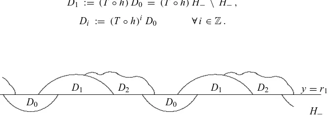
D1 := (T ◦h)D0 = (T◦h)H− \ H−,
Figure 1: Some of the sets Di
We immediately observe that D0⊂H−, while D1⊂R2\H−= {(x,y) : y>r1}. Since(T ◦h)(R2\H−)⊂R2\H−, we can easily conclude that Di ⊂R2\H−for every i ≥ 1. Hence, Di ∩D0 = ∅for every i ≥ 1. This implies that Dk ∩Dj = ∅ whenever j6=k. Since(T ◦h)−1H−⊂H−, we also get Di ⊂H−for every i <0. Furthermore, as T , h and, consequently,(T◦h)are area-preserving homeomorphisms, every Di has the same area in the rolled-up planeR2/ ((x,y)≡(x+2π,y))and its value is 2ε. Thus, as the sets Djare disjoint and contained inR2\H−for every j≥1, they must exhaustAeand hence intersect H+. In particular, there exists n>0 such that
Dn∩H+6= ∅. Since Dn ⊂(T ◦h)nH−, we also obtain that(T◦h)nH−∩H+6= ∅. For such an n >0, we can consider a point Pn ∈ (T ◦h)nH−∩H+with maximal
y−coordinate. The point Pn is not unique, but it exists since, by periodicity, it is sufficient to look at the compact region(T◦h)nH−∩ {(x,y) : 0≤x≤2π , y≥r1}.
In particular, the curveCi runs from Pi−1 to Pi. Furthermore, let us define the curve
C:=C0C1. . .Cn−1Cn. Thus,(T ◦h)(C)=C1C2. . .CnCn+1.
We have constructed a curveCrunning from H−to H+. Now, we will show that it does not pass through any fixed point of h and we will calculate its index. First, we need to list and prove some properties that this curve satisfies.
1. The curveC Cn+1=C0. . .Cn+1has no double points; 2. No point ofChas larger y−coordinate than Pn+1;
In order to prove Property 1, we first observe that asC0has no double points and T ◦h
is a homeomorphism, each curveCi has no double points. Hence, we only need to
show thatCi∩Cj = ∅for every i6= j , exception made for the common endpoint when
|i−j| =1. We initially prove that this is true when i and j are both negative. We recall that the functions f :=(Id+s2) : R −→ Rand f−1are strictly monotone, being
both continuous and bijective. From the positiveness of s2, it immediately follows
that both functions are strictly increasing. Moreover, f−1(x0)≤ x ≤ x0, whenever (x,y)∈C0. Thus, sinceC0⊂H−and since f−1is an increasing function, it turns out that f−2(x0)≤ x ≤ f−1(x0), whenever(x,y)∈ C−1 =h−1(T−1(C0)). In general,
we have
Ci ⊂ {(x,y) : fi−1(x0) ≤ x ≤ f i(x0)} ∀i <0
andCi intersects the boundaries of this strip only in its endpoints (because this is true
forC0and f−1is strictly increasing). Thus,C
l andCs intersect at most in a endpoint, if we choose l and s negative. In general, if we takeCi andCj with i 6= j , then there
exists k<0 such that(T ◦h)ktransforms such curves in two curvesCl andCs with l and s both negative. Finally, the previous step guarantees thatCs∩Cland henceCi∩Cj
are empty, if we exclude the intersection in the common endpoint.
Property 2 is easily proved. In fact, it is immediate to show thatC⊂(T ◦h)nH−. Thus, from the maximal choice involving the y−coordinate of Pn, we can conclude that for every(x,y)∈ C, we obtain y ≤ yn. Moreover, since Pn ∈ H+and Pn+1 = (T ◦h)Pn, we can conclude that yn≤yn+1. This completes the proof of Property 2.
With respect to Property 3, we remark that if we take y ≥ y−1 and if we define (x′,y′) := (T ◦h)(x,y), then y′ ≥ y−1. This is a consequence of the fact that P−1 ∈ H−. Moreover, y0 ≥ y−1 and henceC0 ⊂ {(x,y) : y ≥ y−1}. Thus, for
every(x,y)∈C1=(T ◦h)C0, we get y≥y−1. By induction, Property 3 follows.
Property 1 guarantees thatC does not pass through any fixed point of T ◦h and,
consequently, of h.
We are interested in calculating the index ofC. More precisely, we will show that its value is exactly12. First, we will calculate i(T◦h)(C).
The curveCruns from P−1to Pn. Thus, recalling that(T ◦h) (P−1)= P0and(T ◦ h) (Pn) = Pn+1, let us consider the angleϑ between D(P−1,P0)and D(Pn,Pn+1).
Since, by construction,
P0 = (x0,y0) = (x−1+s2(x−1),y−1+δ2) , 0≤δ2≤ε, Pn+1=(xn+1,yn+1)=(xn−s1(xn),yn+δ1) , 0≤δ1≤ε, then we can write the explicit expression ofϑ
ϑ = π −
arctg
δ1 s1(xn)
+arctg
δ2 s2(x−1)
.
By Property 2 of the index, we can conclude that
i(T◦h)(C) =
ϑ
2π (mod 1)
= 1
2 − 1 2π
arctg
δ1 s1(xn)
+ arctg
δ2 s2(x−1)
From the choice ofε, we get 0 ≤ δi ≤ ε < min si for i ∈ {1,2}. This implies that
belong to the interval [0,π4[. Consequently, 1
Our aim now consists in proving that we can cut mod 1 in the previous formula for
i(T◦h)(C). For this purpose, we will construct a suitable homotopy.
Let P : [−1,0]−→R2be a parametrization ofC0. Setting P(t+1):=(T◦h)(P(t))
for t ∈ [−1,n], we extend the given parametrization of C0 into a parametrization
P : [−1,n+1]−→R2ofC Cn+1. Clearly, if we restrict P to the interval [−1,n],
we obtain a parametrization ofC. Moreover, it is immediate to see that P(i)= Pi for
every integer i∈ {−1,0, . . . ,n+1}. In order to calculate i(T◦h)(C), by definition, we
Of course, in order to evaluate the index we can use P0instead of P.
Now, we are in position to write the required homotopy. We will introduce a family of maps Pλ : [−1,2n+1]−→S1, with 0≤ λ≤n+2. We will define this family
treating separately the cases 0≤λ≤n+1 and n+1≤λ≤n+2.
We develop the first case. The homotopy that we will exhibit will carry the initial map
P0, which deals with the rotation of D(P, (T ◦h)(P))as P moves alongC, into the
This map corresponds to a rotation obtained if we initially move(T ◦h)(P)along
(T ◦h)(C)from(T ◦h)(P−1)=P0to Pn+1, holding P−1fixed, and then we move P
D(P(t0),P(t1))with−1 ≤ t0 < t1 ≤ n +1. By Property 1 ofC, we deduce that
The map Pn+2corresponds to a rotation obtained if we initially move(T◦h)(P)along
the straight line segment P′from P0to Pn+1, holding P−1fixed, and then if we move
with (10) and (11), respectively.
Moreover, the homotopy is well defined. To prove this, we will show first that P(−1)
is never equal to Q := (1−µ)P(t +1)+µP′(t+1)for any t ∈ [−1,n]. Indeed,
by Property 3 ofC, we deduce that Q has larger y−coordinate than P(−1), except possibly when t = −1 orµ=0. However, in both these cases Q=P(t+1)for some
t ∈ [−1,n]. Since in this interval t+1 ≥0 > −1, then Property 1 ofC guarantees that P(t+1)6= P(−1). Hence, P(−1)6=Q.
Analogously, by applying Property 2 and Property 1 of C, we can conclude that
(1−µ)P(t−n−1)+µP′′(t −n −1)6= P(n +1). Thus, the homotopy is well defined.
In particular, Pn+2defined in the interval [−1,2n+1] describes an increase in the
angle which corresponds exactly toϑ, calculated above. Thus as a consequence of the homotopy property, we conclude that
i(T◦h)(C) =
In particular, T0=Id and T1=T . Arguing as before, we can easily see that
(12) i(Ts◦h)(C) =
1 2 −
1 2π
arctg
sδ1 s1(xn)
+arctg
sδ2 s2(x−1)
(mod 1) .
Since this congruence becomes an equality in the case s = 1, by the continuity of the index we infer that also the congruence in (12) is an equality for every s ∈[0,1]. Hence, when s=0 we can conclude that
(13) ih(C) =
1 2.
In order to get the contradiction with Lemma 1, we need to construct another curve
C′running from H
−to H+, having index different from 12. To this aim, we can repeat
the whole argument replacing h with h−1. Now everything works as before except the fact that the directions along which the two boundaries ofAemove under h and under
h−1are opposite. In such a way, we find a curveCbfrom H−to H+with ih−1(Cb)= −
1 2. Let us defineC′ :=h−1
◦Cb: H− −→ H+. By Property 4 of the index, we finally
infer
ih C′
= ih−1 h C′
= ih−1(Cb) = −
1 2.
If we compare the above equality with the equality in (13), we get the desired contra-diction with Lemma 1.
As a consequence of the above proof, Neumann in [27] provides the following useful remark
REMARK 3. If h satisfies all the assumptions of Theorem 7 and it has a finite number of families of fixed points(finite number of fixed points in [0,2π]×[r1,r2]),
then there exist fixed points with positive and negative indices.
We recall that the definition of index of a fixed point coincides with ih(α)for a small circleαsurrounding the fixed point when it has a positive (counter-clockwise) direction. Given a fixed point F, we will denote by i nd(F)its index.
Proof. Let us denote by Fi (i = 1,2, . . . ,k) the distinct fixed points in [0,2π]×
(r1,r2), belonging to different periodic families. Theorem 7 guarantees that k≥2.
It is not restrictive to assume that Fi ∈ (0,2π )×(r1,r2)since we suppose that the
number of families of fixed points is finite. As in the proof of Theorem 7, we extend the homeomorphism h to an homeomorphism in the wholeR2, and we still denote it by h.
If we fix r0<r1, arguing as in the proof of Lemma 1, we can construct a loopD′ :=
D1D2D3D4∈π1(R2\Fix(h), (0,r0)), where
D1covers [0,2π]× {r0}, moving horizontally from(0,r0)to(2π,r0);
D3covers [0,2π]× {r3}, moving horizontally from(2π,r3)to(0,r3); D4covers{0} ×[r0,r3], moving vertically from(0,r3)to(0,r0).
In particular,D′moves with a positive orientation and, by construction, the only fixed points of h it surrounds are exactly the fixed points Fi, i ∈ {1, . . . ,k}. We note that
ih(D1) = ih(D3) = 0, since the curvesD1 andD3 respectively lie in H−and H+ and D(P,h(P))is constant in these regions. Furthermore, being h(x,y)−(x,0)a 2π−periodic function in its first variable, it follows that ih(D4) = −ih(D2). Thus,
Property 3 of the index guarantees thatD′has index zero.
We recall that the fundamental groupπ1(R2\Fix(h), (0,r0))is generated by paths
which start from(0,r0), run along a curveC0 to near a fixed point, loop around this
fixed point and return by−C0 to(0,r0). It is possible to show that the generating
paths, whose composition is deformable into the closed curveD′, surround only the inner fixed points Fi. Consequently, the following equality holds
(14) 0 = ih(D′) =
k
X
j=1
i nd(Fj) .
This means that the sum of the fixed point indices is zero. We remark that such a result could have been directly obtained from the Lefschetz fixed point theorem.
Next step consists in constructing two curves with opposite indices, running from
H−to H+and not passing through any fixed point of h.
Since the number of fixed points in [0,2π]×[r1,r2] is finite, it is possible to consider a non-empty vertical stripWb =[α, β]×R, for someα, β ∈ (0,2π ), which does not contain any Fi. Let us extend 2π−periodicallyW into the setb
[
m∈Z
b
W+(2mπ,0):= {(x,y)∈R2: 2mπ+α≤x≤2mπ+β, m∈Z},
that we still denote byW .b
Arguing as in the proof of Theorem 7, we can find a positive constantε <min si for every i ∈ {1,2}, satisfyingε <kP−h(P)kfor every P∈W . Let us now introduceb
the area-preserving homeomorphismbT : R2−→R2by setting
b
T|[0,2π]×R(x,y):=
(x,y + εcos
π
2(β−α)(2x−β−α)
for x ∈[α, β]
(x,y) otherwise.
Fixed points ofbT ◦h coincide with the ones of h inR2. If we proceed exactly as in the proof of Theorem 7, considering the homeomorphismT instead of T and the setb Wb
instead of W , we are able to construct a curveCof index12, which runs from P−1∈H− to Pn∈ H+and does not pass through any fixed point of h. Analogously, we can find another curveC′of index−1
2running from P−′1∈H−to Pn′∈ H+.
Let us consider now the closed curveF :=C B(−C′)B′, whereBis the straight
particular,Blies in H+and connects the curveCto the curve−C′; whileB′lies in H − and connects the curve−C′to the curveC.
Since, by construction,BandB′have index equal to zero, we infer from Property 2 of the index that
ih(F) = ih(C) −ih(C′) = 1 2 −
−1
2
= 1.
Moreover, the loopF belongs to the fundamental groupπ1(R2\Fix(h),P−1) and
surrounds a finite number of fixed points. Each of them is of the form Fi+m(2π,0)for some i ∈ {1,2. . . ,k}and some integer m∈Z. Since i nd(Fi +m(2π,0))=i nd(Fi) for every m∈Z, we can deduce that
(15) 1 = ih(F) =
k
X
j=1
ν(F,Fj)i nd(Fj) ,
where the integerν(F,Fj)coincides with the sum of all the signs corresponding to the directions of every loop in whichFcan be deformed in a neighbourhood of every point of the form Fj+m(2π,0)surrounded byF. From (15), we infer that there exists
j∗∈ {1,2. . . ,k}such thatν(F,Fj∗)i nd(Fj∗) >0 and, consequently, i nd(Fj∗)6=0.
Hence, recalling that the sum of the fixed point indices is zero (cf. (14)), we can conclude the existence of at least a fixed point with positive index and a fixed point with negative one. This completes the proof.
3. Applications of the Poincar´e-Birkhoff theorem
In this section we are interested in the applications of the Poincar´e-Birkhoff fixed point theorem to the study of the existence and multiplicity of T -periodic solutions of Hamil-tonian systems, that is systems of the form
(16)
x′ = ∂∂Hy(t,x,y)
y′ = −∂∂Hx(t,x,y)
where H :R×R2−→Ris a continuous scalar function that we assume T−periodic in t and C2in z=(x,y).
Under these conditions uniqueness of Cauchy problems associated to system (16) is guaranteed. Hence for each z0 =(x0,y0)∈R2and t0 ∈Rthere is a unique solution (x(t),y(t))of system (16) such that
(17) (x(t0),y(t0))=(x0,y0):=z0.
In the following we will denote such a solution by
For simplicity we set z(t;z0) := (x(t;z0),y(t;z0)) := (x(t;0,z0),y(t;0,z0)). If we suppose that H satisfies further conditions which imply global existence of the solutions of Cauchy problems, then the Poincar´e operator
τ : z0=(x0,y0)→(x(T;(x0,y0)),y(T;(x0,y0)))
is well defined inR2and it is continuous. Also fixed points of the Poincar´e operator are initial conditions of periodic solutions of system (16) and as a consequence of the Liouville theorem, the Poincar´e operator is an area-preserving map. Hence it is natural to try to apply the Poincar´e-Birkhoff fixed point theorem in order to prove the existence of periodic solutions of the Hamiltonian systems.
Before giving a version of the Poincar´e-Birkhoff fixed point theorem useful for the applications, we previously introduce some notation.
Let z : [0,T ] → R2 be a continuous function satisfying z(t) 6= (0,0)for every
t ∈ [0,T ] and(ϑ(·),r(·))a lifting of z(·)to the polar coordinate system. We define the rotation number of z, and denote it by Rot(z)as
Rot(z) := ϑ(T) −ϑ(0)
2π .
Note that Rot(z)counts the counter-clockwise turns described by the vector−−−→0 z(s)
as s moves in the interval [0,T ]. In what follows, we will use the notation Rot(z0)to
indicate Rot(z(·;z0)).
From the Poincar´e-Birkhoff Theorem 4, we can obtain the following multiplicity result.
THEOREM8 ([29]). LetA⊂R2
\{(0,0)}be an annular region surrounding(0,0) and let C1and C2be its inner and outer boundaries, respectively. Assume that C1is strictly star-shaped with respect to(0,0)and that z(·;t0,z0)is defined in [t0,T ] for every z0∈C2and t0∈[0,T ]. Suppose that
i) z(t;t0,z0)6=(0,0) ∀t0∈[0,T [, ∀z0∈C1 , ∀t ∈[t0,T ]; ii) there exist m1, m2∈Zwith m1≥m2such that
Rot(z0) >m1 ∀z0∈C1,
Rot(z0) <m2 ∀z0∈C2.
Then, for each integer l with l ∈ [m2,m1], there are two fixed points of the Poincar´e
map which correspond to two periodic solutions of the Hamiltonian system having l as T−rotation number.
Sketch of the proof. The idea of the proof consists in applying Theorem 4 to the
area-preserving Poincar´e mapτ : z0 −→z(T;z0), considering different liftings of it. For
Since z(t;z0)6=(0,0)for every t ∈[0,T ] and for every z0 ∈A, the liftings are well
defined. We note that as a consequence of i),(0,0)belongs to the image of the interior of C1and also that
Rot(z0) −l≥Rot(z0) −m1 > 0 ∀z0∈C1,
Rot(z0) −l≤Rot(z0) −m2 < 0 ∀z0∈C2.
Hence we can easily conclude that assumptions (a) and (b) in Theorem 4 are satisfied. Moreover it is easy to show that also assumption (c) is verified. Hence, from Theorem 4 we infer the existence of at least two fixed points(ϑli,rli), i = 1,2, ofeτl whose images zliunder the projection5are two different fixed points ofτ. Since(ϑli,rli)are fixed points ofeτl, we get that Rot(zli)=l for every i ∈ {1,2}. We can finally conclude that z(·;z1l)and z(·;zl2)are the searched T−periodic solutions.
There are many examples in the literature of the application of the Poincar´e-Birkhoff theorem in order to study the existence and multiplicity of T−periodic so-lutions of the equation
(18) x′′ + f(t,x) = 0,
with f : R2 −→ R continuous and T -periodic in t. Note that if we consider the
system
(19)
(
x′(t) = y(t)
y′(t) = −f(t,x(t)),
this system is a particular case of system (16) and its solutions give rise to solutions of equation (18). Hence we can consider equation (18) as a particular case of an Hamil-tonian system and everything we mentioned above holds for the case of this equation.
Among the mathematicians who studied existence and multiplicity of periodic so-lutions for equation (18) via the Poincar´e-Birkhoff theorem, we quote Jacobowitz [22], Hartman [20], Butler [7]. We remark that in order to reach the results, in all of these papers the authors assumed the validity of the condition f(t,0)≡0.
With respect to the particular case of the nonlinear Duffing’s equation
x′′ + g(x) = p(t),
we mention the papers [15], [11], [13], [12], [17], [32], in which the Poincar´e-Birkhoff theorem was applied in order to prove the existence of periodic solutions with pre-scribed nodal properties. Among the applications of the Poincar´e-Birkhoff theorem to the analysis of periodic solutions to nonautonomous second order scalar differential equations depending on a real parameter s, we refer to the paper [10] by Del Pino, Man´asevich and Murua, which studies the following equation
and also the paper [30] by Rebelo and Zanolin, which deals with the equation
x′′ + g(x) = s +w(t,x).
Finally, we quote Hausrath, Man´asevich [21] and Ding, Zanolin [14] for the treatment of periodically perturbed Lotka-Volterra systems of type
(
x′ = x(a(t) −b(t)y)
y′ = y(−d(t)+ c(t)x).
We describe now recent results obtained in [24] in which a modified version of the Poincar´e-Birkhoff fixed point theorem is obtained and applied, together with the classical one, in order to obtain existence and multiplicity of periodic solutions for Hamiltonian systems. In their paper the authors study system (16) assuming that z = 0 is an equilibrium point, i.e. Hz′(t,0) ≡ 0, and that it is an asymptotically linear Hamiltonian system. This implies that it admits linearizations at zero and infinity. More precisely, as Hz′(t,0)≡0, if we consider the continuous and T−periodic function with range in the space of symmetric matrices given by t→ B0(t):=Hz′′(t,0), t ∈R, we have
J Hz′(t,z) = J B0(t)z + o(kzk), when z→0.
Moreover, by definiton of asymptotically linear system, there exists a continuous,
T−periodic function B∞(·)such that B∞(t)is a symmetric matrix for each t ∈ R, satisfying
J Hz′(t,z) = J B∞(t)z +o(kzk), when kzk → ∞.
We remark that system (16) can be equivalently written in the following way (20) z′ = J Hz′(t,z) , z = (x,y) , J =
0 1
−1 0
.
Before going on with the description of the results obtained in [24], we recall some results present in the literature dealing with the study of asymptotically linear Hamil-tonian systems.
In [2] and [3], Amann and Zehnder considered asymptotically linear systems inR2N of the form of system (20) with
sup t∈[0,T ],z∈R2N
kHz′′(t,z)k < +∞
and which admit autonomous linearizations at zero and at infinity
z′=J B0z, z′=J B∞z,
remarked that in the planar case N =1 the condition i > 0 corresponds to the twist condition in the Poincar´e-Birkhoff theorem.
Some years later, Conley and Zehnder studied in [9] Hamiltonian systems with bounded Hessian, considering the general case in which the linearized systems at zero and at infinity
z′ = J B0(t)z and z′ = J B∞(t)z
can be nonautonomous. The authors assumed nonresonance conditions for the lin-earized systems at zero and at infinity. Hence, after defining the Maslov indices associ-ated to the above linearizations at zero and infinity, denoted respectively by iT0 and i∞T , they proved the following result.
THEOREM 9. If i0T 6= iT∞, then there exists a nontrivial T−periodic solution of z′= J Hz′(t,z). If this solution is nondegenerate, then there exists another T−periodic solution.
Note that in this last theorem the existence of more than two solutions is not guar-anteed, even if|iT0 −i∞T |is large. This is in contrast with the fact that in the paper [9] and for the case N =1 the authors mention that the Maslov index is a measure of the twist of the flow. In fact, if this is the case, a large|iT0−i∞T |should imply large gaps between the twists of the flow at the origin and at infinity. Hence, the Poincar´e-Birkhoff theorem would provide the existence of a large number of periodic solutions.
The main goal in [24] consists in clarifying the relation between iT0, iT∞and the twist condition in the Poincar´e-Birkhoff theorem, when N =1, obtaining multiplicity results in the case when|i0T −i∞T |is large.
Now we give a glint of the notion of Maslov index in the plane. We will follow [1] (see also [19]).
Let us consider the following planar Cauchy problem
(21)
(
z′ = J B(t)z
z(0) = w,
where B(t)is a T -periodic continuous path of symmetric matrices. The matrix9(t)
is called the fundamental matrix of the system (21) if it satisfies9(t) w = z(t;w). Clearly,9(0)=Id. Moreover, it is well known that as B(t)is symmetric, the funda-mental matrix9(t)is a symplectic matrix for each t ∈[0,T ]. We recall that a matrix A of order two is symplectic if it verifies
(22) AT J A = J,
where J is as in (20). Since we are working in a planar setting, condition (22) is equivalent to
det A = 1,
We will show that, under a nonresonance condition on (21), it is possible to associate to the path t →9(t)of symplectic matrices with9(0)=Id an integer, the T−Maslov index iT(9).
The system z′ = J B(t)z is said to be T−nonresonant if the only T -periodic solution
it admits is the trivial one or, equivalently, if
det(Id−9(T)) 6= 0,
where9is the fundamental matrix of (21).
Before introducing the Maslov indices, we need to recall some properties of Sp(1). If we take A∈Sp(1), then A can be uniquely decomposed as
A =P·O,
where P ∈ {eP ∈ Sp(1) : P is symmetric and positive definitee } ≈ R2 and O is symplectic and orthogonal. In particular, O belongs to the group of the rotations
S O(2) ≈ S1. Thus we can conclude that
Sp(1) ≈ R2×S1 ≈ {z∈R2 : |z|<1} ×S1 = the interior of a torus.
Hence, as [0,1)×R×Ris a covering space of the interior of the torus, we can parametrize Sp(1)with(r, σ, ϑ)∈[0,1)×R×R. In [1] a parametrization
8 : [0,1)×R×R −→ Sp(1)
(r, σ, ϑ) → 8(r, σ, ϑ)=P(r, σ )R(ϑ)
is given, whereϑ is the angular coordinate on S1 and (r, σ ) are polar coordinates in{z ∈ R2 : |z| < 1}. In such a parametrization, for each k ∈ Z andσ ∈ R,
8(0, σ,2kπ )=Id and8(0, σ,2(k+1)π )= −Id (for the details see [1]). The follow-ing sets are essential in order to define the T−Maslov index:
Ŵ+ : = {A∈ Sp(1) : det(Id−A) > 0} = 8{(r, σ, ϑ) : r < sin2ϑ and |ϑ|< π
2 or |ϑ| ≥
π
2},
Ŵ− := {A∈ Sp(1) : det(Id−A) < 0} =8{(r, σ, ϑ) : r > sin2ϑ and |ϑ|< π
2},
Ŵ0 := {A∈Sp(1) : det(Id−A) = 0} =8{(r, σ, ϑ) : r = sin2ϑ and |ϑ|< π
2}. The setŴ0is called the resonant surface and it looks like a two-horned surface with a singularity at the identity.
Now we are in position to associate to each path t →9(t)defined from [0,T ] to Sp(1), satisfying9(0)=Id and9(T)6∈Ŵ0an integer which will be called the Maslov index of9. To this aim we extend such a path t→9(t)∈ Sp(1)in [T,T+1], without intersectingŴ0and in such a way that
• 9(T+1)is a standard matrix withϑ=0, if9(T)∈Ŵ−.
We define the T -Maslov index iT(9)as the (integer) number of half turns of9(t)in
Sp(1), as t moves in [0,T+1], counting each half turn±1 according to its orientation. In order to compare Theorem 8 with Theorem 9 it is necessary to find a character-ization of the Maslov indices in terms of the rotation numbers. To this aim, in [24] a lemma which provides a relation between the T−Maslov index of system
(23) z′ = J B(t)z
and the rotation numbers associated to the solutions of (23) was given.
LEMMA 2. Let9 be the fundamental matrix of system(23)and let iT andψ be,
respectively, its T -Maslov index and the Poincar´e map defined by
ψ : w → 9(T)w .
Consider the T−rotation number Rotw(T)associated to the solution of(23)satisfying
z(0)=w∈S1. Then,
a) iT = 2ℓ+1 withℓ∈Zif and only if deg(Id−ψ,B(1),0)=1 andℓ < min
w∈S1Rotw(T) ≤ wmax∈S1Rotw(T) < ℓ +1;
b) iT = 2ℓwithℓ∈Zif and only if
deg(Id−ψ,B(1),0)= −1 andℓ−1
2 <wmin∈S1Rotw(T)≤wmax∈S1Rotw(T) < ℓ+
1 2;
moreover, in this case there arew1,w2∈S1such that
Rotw1(T) < ℓ < Rotw2(T) .
In the statement of Lemma 2 the T−rotation number Rotw(T)associated to the
solution of(23)with z(0) = w ∈ S1 was considered. We observe that from the linearity of system(23)it follows that Rotw(T)=Rotλw(T)for everyλ >0.
Now, we are in position to make a first comparison between Theorem 8 and Theorem 9.
Let us consider the second order scalar equation
(24) x′′ +q(t,x)x = 0,
where the continuous function q : R×R−→Ris T−periodic in its first variable t and it satisfies
(25) q(t,0) ≡ q0 ∈ R and lim
uniformly with respect to t ∈ [0,T ]. Hence, the linearizations of (24) at zero and
infinity are respectively x′′+q0x =0 and x′′+q∞x =0. We observe that equation (24) can be equivalently written in the following form
x′
y′ !
= y
−q(t,x)x !
= J q(t,x)x y
! .
Analogously, the corresponding linearizations at zero and infinity are given respec-tively by
z′ = J q0 0
0 1
!
z = 0 1
−q0 0 !
z
and
z′ = J q∞ 0
0 1
!
z = 0 1
−q∞ 0
! z.
If we choose q0 = −12 and q∞ = 5, we can easily deduce that there exists r0 > 0
such that Rotw(T) ∈ (−12,12)for everykwk = r0 and there exists R0 > r0 such
that Rotw(T) ∈ (−3,−2)for everykwk = R0. Hence applying Theorem 8 we can
guarantee the existence of four nontrivial T -periodic solutions to equation (24). On the other hand, since iT0 =0 and iT∞ = −5, Theorem 9 ensures the existence of at least one periodic solution.
We recall that, even if the gap between q0and q∞is large, Theorem 9 guarantees only the existence of at least one solution (or at least two solutions if the first one is nondegenerate) while it is quite clear that the number of nontrivial periodic solutions we can find by applying Theorem 8 depends on the gap between q0and q∞.
On the other hand, there are particular situations in which Theorem 9 can be ap-plied, while Theorem 8 cannot, because the twist condition is not satisfied.
For instance, let us set q0 = −12 and q∞ = 12. The corresponding indices are
different, since iT0 = 0, as before, and iT∞= −1. Hence, from Theorem 9, we know that there exists a periodic solution of (24). As far as the rotation numbers are con-cerned, one can prove the existence of R0>r0such that Rotw(T)∈(−1,0)for every
kwk = R0; while, from Lemma 2, there existw1, w2∈R2withkwik =r0(i =1,2)
such that−12 <Rotw1(T) < 0 <Rotw2(T) <
1
2. Consequently, the twist condition
is not verified and Theorem 8 is not applicable. In [24] the authors tried to sharpen the results obtained via the Poincar´e-Birkhoff theorem in order to obtain periodic so-lutions in cases like this one. For this purpose, they developed a suitable version of the Poincar´e-Birkhoff theorem. Before describing this result we can obtain a first result of multiplicity of T -periodic solutions for system (16) which is a consequence of Lemma 2 and of Theorem 8.
We will use the notation: for each s ∈ R, we denote by⌊s⌋the integer part of s, while we denote by⌈s⌉the smallest integer larger than or equal to s.