E l e c t ro n ic
Jo u r n
a l o
f P
r o b
a b i l i t y
Vol. 6 (2001) Paper no. 20, pages 1–21. Journal URL
http://www.math.washington.edu/˜ejpecp/ Paper URL
http://www.math.washington.edu/˜ejpecp/EjpVol6/paper20.abs.html WEAK SOLUTIONS FOR A SIMPLE HYPERBOLIC SYSTEM
Owen D. Lyne
School of Mathematical Sciences, University of Nottingham University Park, Nottingham NG7 2RD, United Kingdom
David Williams
Brookside, Reynoldston, Swansea SA3 1AD, United Kingdom [email protected]
Abstract The model studied concerns a simple first-orderhyperbolic system. The solutions in which one is most interested have discontinuities which persist for all time, and therefore need to be interpreted as weak solutions. We demonstrate existence and uniqueness for such weak solutions, identifying a canonical ‘exact’ solution which iseverywheredefined. The direct method used is guided by the theory of measure-valued diffusions. The method is more effective than the method of characteristics, and has the advantage that it leads immediately to the McKean representation without recourse to Itˆo’s formula.
We then conduct computer studies of our model, both by integration schemes (which do use characteristics) and by ‘random simulation’.
Keywords Weak solutions. Travelling waves. Martingales. Branching processses AMS subject classification 35L45; 60J27; 60G44
Research conducted while both authors were at the University of Bath.
1
Introduction
After a change of the original notation withu replacing 1−u, the FKPP equation (Fisher [6], Kolmogorov, Petrovskii & Piskunov [9]) reads:
∂u ∂t =
1 2
∂2u ∂x2 +u
2−u, u(0, x) =f(x).
McKean [12, 13] showed that one can prove existence and uniqueness results for certain [0, 1]-valued solutions by using martingales to describeuas an explicit functional of a certain branching Brownian motion. He was thereby able to obtain results on convergence to travelling waves for suitable initial dataf. Neveu [15] gives an important completion of McKean’s treatment. Two recent papers — Champneys, Harris, Toland, Warren & Williams [2] and Lyne [10] — have each presented both analytic and probabilistic studies of simple extensions of the FKPP equation. These papers used the probabilist’s golden rule that Itˆo’s formula leads to martingales (see, for example, Rogers & Williams [17]). But the uses of Itˆo’s formula involved the ‘formal generator’ of the branching process in a way which might cause some unease to analysts. The model studied by Lyne concerns a simple first-order hyperbolic system (of similar nature to those studied in Dunbar [4], Othmer, Dunbar & Alt [16], Holmes [8] and Hadeler [7] — see the discussion in Lyne [11] for the relations between the models), a generalization of which we consider here. The solutions in which one is most interested have discontinuities which persist for all time, and therefore need to be interpreted as weaksolutions. Section 2 settles existence and uniqueness for such weak solutions, identifying a canonical ‘exact’ solution which iseverywhere defined. The direct method used is guided by the theory of measure-valued diffusions, MVDs, (see, for example, Dawson [3] and Dynkin [5]). (We stress that no knowledge of MVD theory is assumed here.) The method is more effective than the method of characteristics, and has the advantage that it leads immediately to the McKean representation without recourse to Itˆo’s formula.
Having (we hope) satisfied the requirements of analysis in Section 2, we turn in Section 3 — with more freedom — to the question of computer studies of our model, both by integration schemes (whichdo use characteristics) and by ‘random simulation’. Numerical analysts would wish for more rigour in Section 3. We settle for a certain amount of cross-checking.
Notational point. Weneveruse ut to denote ∂u∂t, ratherut denotesu at timet.
2
Theoretical results
2.1 Our hyperbolic system
LetI be a finite set (with the discrete topology); and letB andR be functions ofI withR≥0. LetQ be anI×I matrix with non-negative off-diagonal elements and zero row sums.
Let f be a Borel function on R ×I with 0 ≤ f ≤ 1. Let u, written (t, x, j) 7→ ut(x, j) and
regarded as a column vector inj when multiplied by Q, be a Borel function on [0,∞)×R×I
with 0≤u≤1. Suppose that u is a weak solution of ∂u
∂t =B ∂u
∂x +Qu+R(u
2−u), “u
In full, the first equation reads:
By the statement that u is a weak solution, we mean that for t > 0 and a test function ϕ ∈ CK1,1,0([0, t]×R×I) (that is a function of compact support, continuously differentiable in [0, t]
2.2 Analytic statement of some results
Shortly we shall shortly reformulate these results probabilistically. Introduce the unique one-parameter (Markov) semigroup {P−R
t : t ≥ 0} acting on Cb(R ×I)
(suffixb standing for ‘bounded’) such that ifh(x, j) =eiθxg(j), where θ∈
R andg is a function
(or column vector) on I, then
t :t≥0}, see the discussion around equation (5) below. By the Riesz representation theorem, {P−R
t : t≥ 0} has a canonical extension to a semigroup on Bb(R ×I), the space of bounded Borel functions on R×I.
Equation (2) implies that for each t >0,u satisfies:
ut=Pt−Rf+
for almost every x. This is proved as follows. Standard Fourier theory shows that forψ0(·,·) in
Then it is almost immediate by the usual Picard/Gronwall argument thatu∗
:= limu(n) exists monotonically and uniformly on each[0, t]×R×I, and so givesthe exactsolution of equation (4):
it is a solution in which there are no ‘exceptional sets’; and if v is another exact solution to equation (4) with 0≤v≤1, then v is equal to u∗
everywhere. Moreover, u∗
is a weak solution of equation (1).
x,j is the measure corresponding to starting position (ξ
0, η0) = (x, j). Let us check that
If we write = to signify equality modulo differentials of local martingales, then (see Rogers &. Williams [17]) In fact, the difference between the integrals of the two sides of equation (6) is bounded on each [0, t], and so is not just a local, but a true, martingale. Hence
d
dt(Stg) =St(iθB+Q−R)g, whereSt is the linear map on vectors on I defined by
Stg:=E
0,jZt(g). Since S0 is the identity, equation (3) now follows.
Guided by McKean, we now construct a branching Markov process related to the hyperbolic equation (1). Time 0 sees the birth of one particle, labelled 1, which has ‘type’ Y1(0) in I and
‘position’ X1(0) in R. At time t ≥ 0, there are N(t) particles which, when labelled in order
of birth, have ‘types’Y1(t), . . . , YN(t)(t) in I, and positions X1(t), . . . , XN(t)(t) in R. The type
of each particle behaves (independently of previous history, of the behaviour of other particles currently alive, etc) as a Markov chain on I with Q-matrix Q. A particle of type j moves on R with constant speed B(j), and gives birth to a new particle of its own type with rate
R(j)h+ o(h). Particles live forever, once born. We write P
x,j and
E
x,j for the probability and expectation corresponding to the situation whenX1(0) =x andY1(0) =j.
We now utilise an obvious argument. Let T be the time of the first birth after time 0, so that T is the birth-time of particle 2. Because of the rˆole of R as birth-rate function, we have
P
From time T on, the family tree of particle 2 evolves independently of its complement in the family tree of particle 1. We therefore have
E we see thatvsatisfies equation (4) exactly. Hence v=u∗
everywhere, and we have the McKean representation
u∗
t(x, j) =E
x,jΠ(t).
2.4 Convergence to travelling waves: the easy case
Condition (†)
We consider the very special situation in which
Q is irreducible and there is a statej0∈I with
B(j0)< B(j) for j6=j0 and for which R(j0)>−Q(j0, j0).
We will refer to these conditions as (†).
When (†) holds there will almost surely exist at some time a particle of typej0 which has an
infinite ‘line of descent’ consisting entirely of particles of typej0. Thus there will be arandom
interval [σ,∞), which we choose to be maximal, such that for some random constantA, L(t)−B(j0)t=A for t∈[σ,∞).
Then
ut(x−B(j0)t, j) = P
0,j(x+L(t)−B(j
0)t >0)
→w(x, j) = P
0,j(A >−x), and w(x+tB(j0), j) is a travelling-wave solution of equation (1).
In this case,
ut(x, j0) = 1 if x >−tB(j0),
ut(x, j0) = 1−P
0,j0
(L(t) =tB(j0))<1 if x=−tB(j0),
and the jumpP
0,j0(L(t) =tB(j
0)) at the ‘characteristic point’x=−tB(j0) converges ast→ ∞
to
P
0,j0
(σ = 0) = R(j0) +Q(j0, j0) R(j0)
.
For numerical and simulation studies of such a case, see section 3 below.
2.5 The difficult cases
It is hoped to make the difficult cases when (†) fails to hold the subject of another paper giving direct proofs for this simple situation of results
ut+ct−a(t)(x, j)→w(x, j) where a(t) =o(t).
3
Numerical analysis
We use both probabilistic simulation of the branching process and finite difference methods (the most effective being upwinding along characteristics) to study the initial value problem for the case where I = {1,2}, that is, we have a pair of coupled first order PDEs (as studied in Lyne [10]). As in Dunbar [4] and Holmes [8], these can be rewritten as a single second order PDE which is a generalization of the telegraph equation. It is convenient to change to moving coordinates (moving at a speed of 12(B(1) +B(2))) and then re-scale time so that the coefficients of ∂u
∂x are 1 and −1. This is possible unless B(1) =B(2) — this case reduces to a pair of first order ODEs and is dealt with by Lyne [10]. For the remainder of this paper, we shall denote ut(x,1) by u(t, x) andut(x,2) byv(t, x) and set B(1) = 1, B(2) =−1. Particularly interesting is Heaviside initial data, that is,
u(0, x) =v(0, x) =
1 ifx >0, 0 ifx≤0.
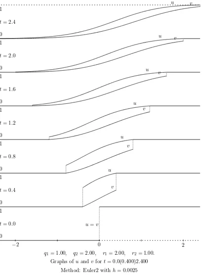
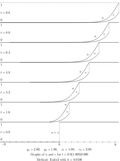
We present first the skeleton of theC program used to produce the numerical solution plotted in Figures 1 and 4. It implements a naive Euler method along the characteristics of the system, and a modification of the Euler method. The figures were produced using the modified method, but output of the two methods is practically indistinguishable.
/* EULER METHODS
This is only part of a program.
Use of naive Euler methods for a simple hyperbolic system
du/dt = du/dx + f(u,v), f(u,v) = q1 (v-u) + r1 u(u-1); dv/dt = -dv/dx + g(u,v), g(u,v) = q2 (u-v) + r2 v(v-1);
with Heaviside initial data
u(0,x) = v(0,x) = 1 for x > 0, 0 for x <= 0.
After the nth step, u[k] = uu[k+500] (‘idioC’!) represents u(nh, 2kh) if n is even;
u(nh, (2k-1)h) if n is odd.
So, as it were, u[n,k] (that is, u[k] after n time steps) corresponds to the pattern
t=2h [2,-1] [2,0] [2,1]
t= h [1,0] [1,1]
t= 0 [0,-1] [0,0] [0,1]
This is suited to integrating along the characteristics, but we have to watch the parity.
nu denotes the next u-array, that is, u one time step later.
We consider the values -480 <= k <= 480; 0 <= n <= 960 (= bign),
with printouts every 160 (=gap) steps. */
#define bign 960 #define gap 160
double q1, q2, r1, r2, t;
int a, b, n; /* a and b are x-values where there are discontinuities */ double uu[1001], vv[1001], nuu[1001], nvv[1001];
double *u= &uu[500]; double *v= &vv[500]; double *nu=&nuu[500]; double *nv=&nvv[500];
int k, j, parity, method; double h;
void Solve(void); /* calls up Display when appropriate */ void Euler1(void); void Euler2(void); double Trim(double z);
void Solve(void) { double temp;
/* Initialize */
for(k=-485; k<= 0; k++) {u[k] = 0.0; v[k] = 0.0;} for(k=1; k<= 485; k++) {u[k] = 1.0; v[k] = 1.0;}
parity=0;
for(n=1; n<=bign; n++)
{ a = 1 - (n/2); b=(n+1)/2; parity = 1 - parity;
for(k=a; k<= b; k++) { j = k + 1 - parity;
(method == 1)? Euler1(): Euler2(); }
/* Stabilize */ for (k=a; k<=b; k++)
{ u[k] = Trim(nu[k]); v[k] = Trim(nv[k]); }
/* Display */
if (n % gap == 0) {t = n * h; Display();} }
}
{ nu[k] = u[j] + h * f(u[j],v[j]);
nv[k] = v[j-1] + h * g(u[j-1], v[j-1]); }
void Euler2(void) /* a refinement of the method */ { double nu_temp, nv_temp;
nu_temp = u[j] + h * f(u[j],v[j]);
nv_temp = v[j-1] + h * g(u[j-1], v[j-1]);
nu[k] = u[j] + 0.5*h*(f(u[j],v[j]) + f(nu_temp, nv_temp)); nv[k] = v[j-1]+0.5*h*(g(u[j-1], v[j-1])+g(nu_temp, nv_temp)); }
double Trim(double z) { if (z>1.0) return 1.0
else if (z<0.0) return 0.0 else return z;
}
/* EOF */
Several finite difference methods were implemented on a rectangular lattice. These all proved to be less effective than the Euler method used along the characteristics (via the customized lattice, that is, using the characteristics to build the grid). The most effective of these schemes was the Lax-Wendroff scheme, as implemented in the following program. Mitchell and Griffiths [14, Chapter 4] give a good discussion of the Lax-Wendroff scheme and hyperbolic equations in general; see also Strikwerda [18].
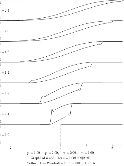
A solution plotted from this program is presented in Figure 3. It is fairly similar to the plots in Figures 1 and 2 for the same parameter values using the other methods investigated, but it suffers from typical Gibbs phenomena, and does not maintain the sharp discontinuities actually present in the true solution along each characteristic. However, for the parameter values given, these discontinuities decay exponentially to zero, and for longer times the solutions of all three methods agree very well. In cases where a discontinuity does not decay to zero (but instead to a finite size between 0 and 1, as in Figures 4 and 5), the Lax-Wendroff method is visibly worse because the discontinuity is smeared out over several grid points. Away from the discontinuity agreement is good.
/* LAX-WENDROFF SCHEME
This is only part of a program.
Use of Lax-Wendroff scheme for a simple hyperbolic system du/dt = du/dx + f(u,v), f(u,v) = q1 (v-u) + r1 u(u-1); dv/dt = -dv/dx + g(u,v), g(u,v) = q2 (u-v) + r2 v(v-1); with Heaviside initial data
u(0,x) = v(0,x) = 1 for x > 0, = 0 for x <= 0.
be below 1 for most of these schemes).
nu denotes the next u-array, that is, u one time step later.
We consider the values -480 <= k <= 480; 0 <= n <= 480 (= bign), with printouts
every 80 (=gap) steps. */
#define gap 80 #define bign 480
double q1, q2, r1, r2, t;
int a, b, n; /* a and b control the region of the array in which calculation is performed, n is the current number of the time steps */
double uu[1001], vv[1001], nuu[1001], nvv[1001]; double *u = &uu[500]; double *v = &vv[500]; double *nu = &nuu[500]; double *nv = &nvv[500];
int k; /* to be used as a counter variable */
double h; double lam; /* lambda = time-step divided by space-step */
void Solve(void); /* calls up Display when appropriate */ double Trim(double z); /* ensures values stay in [0,1] */
void LaxWen(void); /* Lax-Wendroff method */
void Solve(void) {
/* Initialize */
for(k=-485; k<= 0; k++) {u[k] = 0.0; v[k] = 0.0;} for(k=1; k<= 485; k++) {u[k] = 1.0; v[k] = 1.0;} for(n=1; n<=bign; n++) {
a = 1 - n; b = n;
for(k=a; k<= b; k++) {LaxWen();} }
/* Stabilize */ for(k=a; k<=b; k++)
{u[k] = Trim(nu[k]); v[k] = Trim(nv[k]);}
/* Display */
if (n % gap == 0 ) {t = n * h * lam;Display();} }
}
void LaxWen(void)
{ nu[k] = u[k] + 0.5 * lam * (u[k+1] - u[k-1])
+ 0.5*lam*lam*(v[k+1] + v[k-1] - 2*v[k]) + h*lam*g(u[k],v[k]); }
double Trim(double z) { if (z>1.0) return 1.0
else if (z<0.0) return 0.0; else return z;
}
/* EOF */
3.1 Probabilistic simulation
The key to the probabilistic simulation is a simple recursive function calledLife. This function tracks the path of an individual particle, updating the record of the left-most position yet reached by any particle each time the record is broken, and storing in arrays the time, place and type of each birth. Then, upon completion of a particle’s run (since we only run each particle up until a pre-specified maximum time), we check to see if we have any more particles to do, and run theLifefunction on them.
Each particle is dealt with in a series of segments (the function DoSegment). An exponential random variable is generated (byRexp)— the length of time untileitherthe particle splits into two or the particle changes type. The position of the particle is updated by simply adding the length of time multiplied by its speed in its type for the segment to the current position. If the length of the segment takes us past our maximum time, we have completed the life story for that particle, and move on to the next one (incrementingc, the number of our current particle). Then we determine which event it was that did actually occur — birth or mutation. For birth we call the functionCreate, which stores the time, position and type in the arrays tt,xx and yy respectively. We also increment the counter nto inform us there is one more particle to be dealt with later. We then do another segment. If we change type, then we flip the type variable yand do the next segment.
Once we reach a point where we have completed the life story of a particle and there are no more sets of birth information unused (i.e. c greater than n), we have finished the simulation run.
If one is interested in calculating solely, for example, the left-most particle position, much calculation can be saved. Since a particle can only travel at speeds 1 and−1 we have immediate bounds on its future position (and identical bounds on all its future descendants). Thus, if the maximum time we are running until isT and the current record for left-most position isX, we can discard any particle in the simulation (denoting its position and time by (t, x)) for which x−(T−t)> X; particles satisfying this inequality have no chance of changing the record. The fact that their descendants also cannot break the record means we can discard the parent and save even generating the descendants.
/* SIMULATION OF BRANCHING PROCESS MODEL
save some computation if this is all we are interested in (by pruning away particles far away from the left-most).
While in type 1 particle moves at speed b[1] (wlog set to 1), mutates at rate q[1] and breeds at rate r[1] - in type 2 particle moves at speed b[2] (wlog set to -1), mutates at rate q[2] and breeds at rate r[2] - q and r user inputs.
The program notes the position of the left-most particle in each of NUMRUN (1000) simulations starting from 1 particle at the origin (doing 1000 runs for that particle being type 0, and 1000 for type 1), observing each simulation at T (6)
points, each GAP (user input) units apart. */
#define NUMRUN 1000
#define MAXPART 1000000 /* limit on particle numbers, warning if exceeded */ #define T 6
double b[3],Lpos[T+1],tt[MAXPART+1],xx[MAXPART+1],x,GAP,leftu[T+1][NUMRUN], leftv[T+1][NUMRUN],q[3],r[3];
int y,c,yy[MAXPART+1],TYPE,k;
void OneRun(void); void DoSegment(void); void Life(void); void Create(void);
int main() {
int i,j; b[1]=1.0; b[2]=-1.0;
/* Simulations starting from 1 particle of type 1 */ TYPE=1;
for(i=0; i<NUMRUN; ++i) { OneRun();
for(j=0;j<=T;++j) { leftu[j][i]=Lpos[j]; }
}
/* Simulations starting from 1 particle of type 2 */ TYPE=2;
for(i=0; i<NUMRUN; ++i) { OneRun();
for(j=0;j<=T;++j) { leftv[j][i]=Lpos[j]; }
} }
int i;
n=0; c=0; t=0.0; x=0.0; Lpos[0]=x; tt[0]=t; xx[0]=x; yy[0]=TYPE;
for(i=1; i <= T; ++i) { Lpos[i]=10000;
}
Life(); }
double RUnif() /* a different random number generator could go here */ {
double drand48(); return(drand48()); }
double Rexp(lam) double lam; {
double log();
return(-log(RUnif())/lam); }
void DoSegment(void) /* update particles age and position */ {
double e,Rexp(); int i,j;
e=Rexp(q[y]+r[y]); j=t/GAP; k=(t+e)/GAP; if (k > T)
k=T;
for(i = j + 1; i <= k; ++i) {
if (Lpos[i] > x + b[y] * (i * GAP - t)) {
Lpos[i]=x+b[y]*(i*GAP-t); /* this notes any new records set by this particle */ }
}
x += e*b[y]; t += e; }
void Life(void) {
double RUnif();
/* initialise next particle */ t = tt[c]; x = xx[c]; y = yy[c];
while (t < T*GAP && (x+t-(T*GAP)) < Lpos[T]) { DoSegment();
Create(); else
y = 3 - y; /* This sends 1 to 2 and 2 to 1 */ }
c++;
if (c >= MAXPART)
printf("\nFilled up particle arrays\n"); else if (c <= n)
Life(); }
void Create(void) /* a new particle has been born, store its details */
{ n++;
if (n < MAXPART)
{tt[n]=t; xx[n]=x; yy[n]=y;} }
/* EOF */
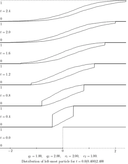
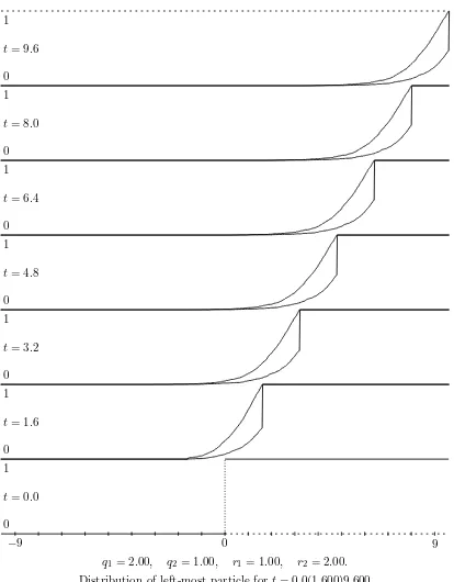
Plots of the solutions obtained by simulation are presented in Figures 2 and 5. These agree very well with those produced by the Euler method for corresponding parameters in Figures 1 and 4. When more simulation is done the probabilistic plots are smoother and agreement is even better. This simulation method could of course easily be extended to then-type case.
3.2 Discussion of figures
Consider the situation in which there is just one particle at time 0, of type 2 and with position x. We know thatv(t, x) is the probability that all particles are to the right of 0 at timet. Since no particle can travel left at speed greater than 1,v(t, x) = 1 forx > t. However, ifx=t, then v(t, t) is the probability that up to timetour initial particle has no line of descent consisting only of particles of type 2: in other words, that every descendant of our initial particle spends some time beforet moving right (in which case it can never get to 0 at time t). It is therefore clear that there is a positive jump 1−v(t, t) inv(t,·) at timet, and that this jump may be calculated by regarding any particle of type 1 as ‘dead’ and ignoring it and its descendants. Precisely, the jump 1−v(t, t) is the probability that a continuous-time branching process starting from 1 particle, and with birth-rate r2 and death-rate q2 (per individual) survives until time t. If
q2 > r2, the situation in Figures 1, 2 and 3, then this survival probability tends exponentially
fast to 0. Ifr2> q2, the situation in Figures 4 and 5, thenv(t, t)→1−π, where the extinction
probability π satisfies
π= q2 q2+r2
+ r2 q2+r2
π2,
so thatπ =q2/r2.
0
0
0
0
0
0
0 0
1
1
1
1
1
1
1 t= 0.0
2 −2
u=v t= 0.4
u
u
u
u
u
u
v
v
v
v
v
v t= 0.8
t= 1.2 t= 1.6 t= 2.0 t= 2.4
q1= 1.00, q2= 2.00, r1= 2.00, r2= 1.00.
Graphs ofu and v fort= 0.0(0.400)2.400 Method: Euler2 with h= 0.0025
0
0
0
0
0
0
0 0
1
1
1
1
1
1
1 t= 0.0
2 −2
t= 0.4 t= 0.8 t= 1.2 t= 1.6 t= 2.0 t= 2.4
q1= 1.00, q2= 2.00, r1= 2.00, r2= 1.00.
Distribution of left-most particle fort= 0.0(0.400)2.400 1000 Runs each from type 1, and from type 2, initial particle
0
0
0
0
0
0
0 0
1
1
1
1
1
1
1 t= 0.0
2 −2
t= 0.4 t= 0.8 t= 1.2 t= 1.6 t= 2.0 t= 2.4
q1= 1.00, q2= 2.00, r1= 2.00, r2= 1.00.
Graphs ofu and v fort= 0.0(0.400)2.400 Method: Lax-Wendroff withh= 0.010, λ= 0.5
0
0
0
0
0
0
0 0
1
1
1
1
1
1
1 t= 0.0
9 −9
u=v t= 1.6
u
u
u
u
u
u
v
v
v
v
v
v t= 3.2
t= 4.8 t= 6.4 t= 8.0 t= 9.6
q1= 2.00, q2= 1.00, r1= 1.00, r2= 2.00.
Graphs ofu and v fort= 0.0(1.600)9.600 Method: Euler2 with h= 0.0100
0
0
0
0
0
0
0 0
1
1
1
1
1
1
1 t= 0.0
9 −9
t= 1.6 t= 3.2 t= 4.8 t= 6.4 t= 8.0 t= 9.6
q1= 2.00, q2= 1.00, r1= 1.00, r2= 2.00.
Distribution of left-most particle fort= 0.0(1.600)9.600 1000 Runs each from type 1, and from type 2, initial particle
follows. Again, consider the situation in which there is just one particle at time 0, of type 2 and with position x. For small t, the dominant contribution to v(t, x) will arise from cases where there is a random timeS beforet at which the particle changes type. Thus the particle moves left for a timeS and right for a timet−S, ending up at x−S+t−S. Thus, for smallt,
v(t, x)≈P(x−S+t−S >0) =P
n
S < 1 2(x+t)
o
= 1−e−1
2q2(x+t) ≈ 1
2q2(x+t).
Acknowledgements. Owen Lyne would like to thank the EPSRC for financial support in the form of a Research Studentship.
References
[1] Bramson, M. D. (1983) Convergence of solutions of the Kolmogorov equation to travelling waves.
Mem. Amer. Math. Soc.,285, 1–190.
[2] Champneys, A., Harris, S., Toland, J., Warren, J. & Williams, D. (1995) Algebra, analysis and probability for a coupled system of reaction-diffusion equations.Phil. Trans. R. Soc. Lond., A350, 69–112.
[3] Dawson, D. A. (1993) Measure-valued Markov processes,Ecole d’ ´´ Et´e de Probabilit´es de Saint Flour, 1991, Lecture Notes in Mathematics,1541. New York: Springer-Verlag.
[4] Dunbar, S. R. (1988) A branching random evolution and a nonlinear hyperbolic equation.SIAM J. Appl. Math,48, 1510–1526.
[5] Dynkin, E. B. (1994)An Introduction to Branching Measure-Valued Processes. Providence, Rhode Island: American Mathematical Society.
[6] Fisher, R. A. (1937) The wave of advance of an advantageous gene.Ann. Eugenics,7, 353–369.
[7] Hadeler, K. P. (1995) Travelling fronts in random walk systems.Forma, 10, 223–233.
[8] Holmes, E. E. (1993) Are diffusion models too simple? A comparison with telegraph models of invasion.Amer. Nat.,142, 779–795.
[9] Kolmogorov, A. N., Petrowski, I. & Piscounov, N. (1937) ´Etude de l’´equation de la diffusion avec croissance de la quantit´e de mati`ere et son application `a un probl`eme biologique.Mosc. Univ. Bull. Math., 1, 1–25.
[10] Lyne, O.D. (2000) Travelling waves for a certain first-order coupled PDE system.Electron. J. Probab.,
5:14, 1–40.
[11] Lyne, O.D. (1996) Probability and analysis for a hyperbolic coupled PDE system. Unpublished Ph.D. thesis, University of Bath.
[12] McKean, H. P. (1975) Application of Brownian motion to the Equation of Kolmogorov-Petrovskii-Piskunov.Comm. Pure Appl. Math.,28, 323–331.
[13] McKean, H. P. (1976) Correction to the above.Comm. Pure Appl. Math.,29, 553–554.
[14] Mitchell, A. R. & Griffiths, D. F. (1980)The Finite Difference Method in Partial Differential Equa-tions. Chichester: Wiley
[16] Othmer, H. G., Dunbar, S. R. & Alt, W. (1988) Models of dispersion in biological systems.J. Math. Biol., 26, 263–298.
[17] Rogers, L. C. G. & Williams, D. (1987)Diffusions, Markov Processes and Martingales, Volume 2: ItoˆCalculus. Chichester: Wiley.
