c
C h a p t e r 2
At this point we have considered discrete sample spaces and derived theorems con-cerning probabilities for any discrete sample space and some of the events within it. Often, however, events are most easily described by performing some operation on the sample points. For example, if two dice are tossed, we might consider the sum showing on the two dice; but when we find the sum, we have operated on the sample point seen. Other operations, as we will see, are commonly encountered.
We want to consider some properties of the sum; we start with the sample space. In this example a natural sample space shows the result on each die and, if the dice are fair, leads to equally likely sample points. The sample space consists then of the 36 points in S1:
S1= {.1;1/; .1;2/; : : : ; .1;6/; .2;1/; : : : ; .6;6/}:
If we consider the sum on the two dice, then a sample space
S2 = {2;3;4;5;6;7;8;9;10;11;12}
might be considered, but now the sample points are not equally likely. We call the sum in this example a random variable.
Definition:A random variable is a real-valued function defined on the points of a sample space.
Various functions occur commonly and we will be interested in a variety of them; sums are among the most interesting of these functions, as we will see. We will soon determine the probabilities of various sums, but the determination of these is probably evident now to the reader. We first need, for this problem as well as for others, some ideas and some notation.
2.1
c
Random Variables
We have considered only discrete sample spaces to this point; we discuss discrete random variables in this chapter.
First consider another example. It is convenient to let X denote the number of times an examination is attempted until it is passed. X in this case denotes a random variable; we will use capital letters to denote random variables. We show some of the infinite sample space here, indicating the value of X;x;at each point.
Event x
P 1
F P 2
F F P 3
F F F P 4
::
2.1 Random Variables 77
Clearly we see that the event ′X=3′is equivalent to the event ′F F P′and so their probabilities must be equal. Therefore,
P.X=3/= P.F F P/= 1 8:
The terminology “random variable” is curious since we could, in the above ex-ample, define a variable, say Y , to be 6 regardless of the outcome of the experiment. Y would carry no information whatsoever, and would be neither random nor variable! There are other curiosities with terminology in probability theory as well, but they have become, alas, standard in the field and so we accept them. What we call here a random variable is in reality a function whose domain is the sample space and whose range is the real line. The random variable here, as in all cases, provides a mapping from the sample space to the real line. While being technically incorrect, the phrase “random variable” seems to convey the correct idea. This perhaps becomes a bit more clear when we use functional notation to define a function f.x/to be
f.x/= P.X=x/;
where x denotes a value of the random variable X:In the example above we could then write f.3/= 18:The function f.x/is called a probability distribution function (abbreviated as pdf ) for the random variable X:
Since probabilities must be non-negative and since the probabilities must sum to 1, we see that
1] f.x/≥0
and
2] P
S f.x/=1 where S is the sample space.
We turn now to some examples of random variables.
Ex ample 2.1.1
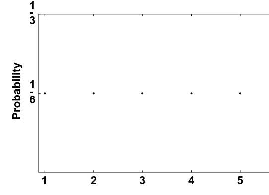
Throw a fair die once and let X denote the result. The random variable X can assume the values 1, 2, 3, 4, 5, 6 and so
P.X =x/= ²1
6 for x =1;2;3;4;5;6 0; otherwise.
A graph of this function is of course flat; it is shown in Figure 2.1. This is an example of a discrete uniform probability distribution.
1 2 3 4 5 6 Face
1 -6 1 -3
Probability
Figure 2 . 1 Discrete uniform probability distribution.
Ex ample 2.1.2
In the previous example the die is fair, so now we consider an unfair die. In particular, could the die be weighted so that the probability a face appears is proportional to the face?
Suppose that X denotes the face that appears and let P.X =x/=k·x where k denotes the constant of proportionality. The probability distribu-tion funcdistribu-tion is then
P.X =x/= 8 > > > > > <
> > > > > :
k if x =1 2k if x =2 3k if x =x 4k if x =4 5k if x =5 6k if x =6
:
The sum of these probabilities must be 1, so k+2k+3k+4k+5k+6k=1, hence k= 211 and the weighting is possible.
The probability distribution function is
P.X =x/= 8 <
: x
[image:4.612.172.443.60.257.2]2.1 Random Variables 79
A procedure for selecting a random sample from this distribution is explained in Appendix 1. b
Ex ample 2.1.3
Now we return to the experiment consisting of throwing two fair dice. We want to investigate the probabilities of the various sums that can occur. Let the random variable X denote the sum that appears. Then, for example,
P.X =5/= P[.1;4/or.2;3/or.3;2/or.4;1/]
= 4
36 = 1 9:
So we have determined the probability of one sum. Others can be deter-mined in a similar way.
The experiment could be described by giving all the values for the probability distribution function (or pdf), P.X =x/;where, as before, x denotes a value for the random variable X;as we saw in Example 2.1.2. In this example, it is easy to find that
P.X =x/=
8 > > > > > > > > > > > > <
> > > > > > > > > > > > : 1
36 if x =2 or 12 2
36 if x =3 or 11 3
36 if x =4 or 10 4
36 if x =5 or 9 5
36 if x =6 or 8 6
36 if x =7 0; otherwise. We see that
P.X =x/= P.X =14−x/= x −1
36 for x =2;3;4;5;6;7 and
P.X =x/=0; otherwise.
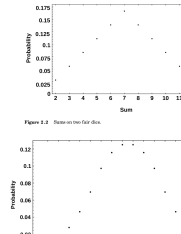
A graph of this function shows a tent-like shape, as in Figure 2.2. b
2 3 4 5 6 7 8 9 10 11 12 Sum
0 0.025 0.05 0.075 0.1 0.125 0.15 0.175
Probability
Figure 2 . 2 Sums on two fair dice.
3 4 5 6 7 8 9 10 11 12 13 14 15 16 17 18
Sum 0
0.02 0.04 0.06 0.08 0.1 0.12
Probability
Figure 2 . 3 Sums on three fair dice.
[image:6.612.126.488.66.534.2]2.1 Random Variables 81
A natural inquiry at this point is, “What is the probability distribution of the sum on three fair dice?” It is more difficult to work out the distribution here than it was for two dice. While we will show another solution later, we give one approach to the problem at this time. Consider, for example, a sum of 10 on three dice. The sum could have arisen from these combinations of results showing on the individual dice (which do not indicate which die showed which face):
.2;2;6/; .3;3;4/; .2;4;4/; .3;1;6/; .3;2;5/; .5;1;4/:
Each of the first three of these combinations could occur in 3 different orders (corresponding to the three different dice), while each of the last three could occur in 6 different orders. This gives a total of 27 possibilities, each of which has probability2161 . Therefore P.X=10/= 21627. A similar process could be followed for other values of the sum; the complete probability distribution can be found to be
P.X=x/= 8 > > > > > > > > > > > > > > > > > > < > > > > > > > > > > > > > > > > > > : 1
216 if x=3 or 18 3
216 if x=4 or 17 6
216 if x=5 or 16 10
216 if x=6 or 15 15
216 if x=7 or 14 21
216 if x=8 or 13 25
216 if x=9 or 12 27
216 if x=10 or 11 0; otherwise.
A computer algebra system may also be used to find the probability distribution for X:Many systems will give all the permutations, each of which may be summed and the relative frequencies recorded. This is shown in Appendix 1. There are other methods that can be used to solve the problem; one of these will be discussed in Chapter 4.
A graph of this function is shown in Figure 2.3. It begins to show what we will call a normal probability distribution shape. As the number of dice increases, the “curve” the eye sees smooths out to resemble a normal probability distribution; the distribution for six or more dice is remarkably close to the normal distribution. We will discuss the normal distribution in Chapter 3.
Ex ample 2.1.4
If P.X =i/ is denoted by Pi, for i =1;2;3;4;5;6; and if k is the constant of proportionality, then P12=2k, 2 P1P2 =3k, 2 P1P3+P22
=4k, and so on, together with the restriction thatP6i=1Pi =1, giving a system of 12 equations in 7 unknowns. Unfortunately this set of equations has no solution, so we can’t load the die in the manner suggested. b
Ex ample 2.1.5
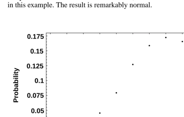
Let’s look now at the sum when two loaded dice are thrown. First let each die be loaded so that the probability a face occurs is proportional to that face, as in Example 2.1.2. The sample space of 36 points can be used to determine the probabilities of the various sums. Figure 2.4 shows these probabilities. We see that the symmetry we noticed in Figures 2.1 and 2.3 is now gone.
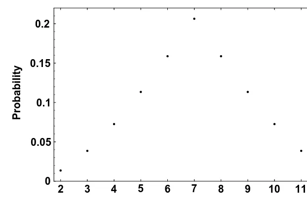
Now suppose one die is loaded so that the probability a face appears is proportional to that face, while a second die is loaded so that the probability face i appears is proportional to 7−i; i =1;2; : : : ;6:The probabilities of various sums are shown in Figure 2.5. Now symmetry around x =7 has returned.
The appearance, once more, of the normal-like shape is striking. Read-ers with access to a computer algebra system may want to find the proba-bility distribution of the sums on four dice, two loaded in each manner as in this example. The result is remarkably normal. b
2 3 4 5 6 7 8 9 10 11 12
Sum 0
0.025 0.05 0.075 0.1 0.125 0.15 0.175
Probability
[image:8.612.152.463.381.579.2]2.1 Random Variables 83
2 3 4 5 6 7 8 9 10 11 12
Sum 0
0.05 0.1 0.15 0.2
Probability
Figure 2 . 5 Sums on two loaded dice.
Ex ample 2.1.6
Sample spaces in the examples in this chapter so far have been finite. Our final example involves a countably infinite sample space. Consider observing single births until a girl is born. Let the random variable X denote the number of births necessary. Assuming the births to be independent,
P.X =x/=
1 2
x
; x =1;2;3; : : : :
To check that P.X =x/ is a probability distribution, note that P.X =x/≥0 for all x:The sum of all the probabilities is
S = ∞ X
x=1
P.X =x/=
1 2
+
1 2
2
+
1 2
3
+ · · ·:
To calculate this sum, note that
1 2
S=
1 2
2
+
1 2
3
+
1 2
[image:9.612.162.473.56.263.2]Subtracting the second series from the first gives
1 2
S =
1 2
so S=1:
Another way to sum the series is to recognize that it is an infinite geometric series of the form
S=a+ar +ar2+ · · · and the sum of this series is known to be
S = a
1−r; if|r|<1: In this case a is 12 and r is also 12;so the sum is 1.
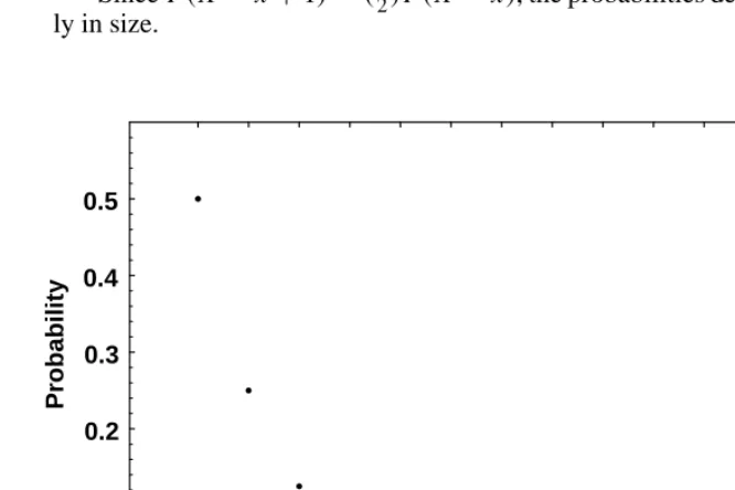
Here X is called a geometric random variable. A graph of P.X =x/ appears in Figure 2.6.
Since P.X =x+1/=.12/P.X =x/, the probabilities decline
rapid-ly in size. b
1 2 3 4 5 6 7 8 9 10 11 12 13 14 X
0 0.1 0.2 0.3 0.4 0.5
Probability
[image:10.612.141.474.375.597.2]2.2 Distribution Functions 85
2.2
c
Distribution Functions
Another function often useful in probability problems is called the distribution function. For a discrete random variable we denote this function by F.x/where
F.x/= P.X ≤x/;
so F.x/= P
t≤x
f.t/:
F.x/is also known as a cumulative distribution function (abbreviated cdf ) because it accumulates probabilities. Note the distinction now between f.x/, the probability distribution function (pdf), and F.x/, the cumulative distribution function (cdf).
In Chapter 1 we used the reliability of a component where R.t/= P.T >t/, so
R.t/=1−F.t/;
establishing a relationship between R.t/and the distribution function.
Ex ample 2.2.1
For the fair die whose probability distribution function is given in Example 2.1.1, we find
F.1/= 1
6;F.2/= 2
6;F.3/= 3
6;F.4/= 4
6;F.5/= 5
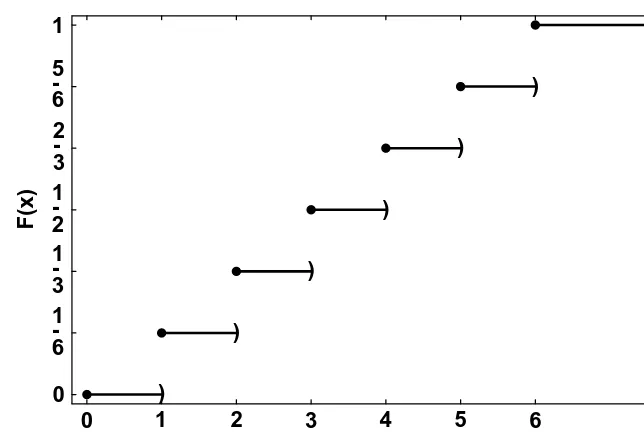
6;F.6/=1: It is also customary to show this function for any value of the random variable X. Here, for example, F.3:4/= P.X ≤3:4/= 36:Since F.x/is defined for any value of X;we draw a continuous graph, unlike the graph of the probability distribution function. We see that in this case,
F.x/= 8 > > > > > > > > > > > <
> > > > > > > > > > > :
0; if x <1 1
6; if 1≤x <2 2
6; if 2≤x <3 3
6; if 3≤x <4 4
6; if 4≤x <5 5
6; if 5≤x <6 1; if 6≤ x
:
0 1 2 3 4 5 6 Face
0 1 -6 1 -3 1 -2 2 -3 5 -6 1
F(x)
)
)
)
)
)
)
Figure 2 . 7 Distribution function for one toss of a fair die.
It is clear from the definition of F.x/and from the fact that probabilities are in the interval [0,1] that
0≤ F.x/≤1 and that
F.a/≥ F.b/if a≥ b.
It is also true, for discrete random variables taking integer values, that P.a≤ X ≤b/= P.X ≤b/−P.X <a/= F.b/−F.a−1/: Individual probabilities, say P.X =a/;can be found by
P.X =a/= P.X ≤a/−P.X ≤a−1/= F.a/−F.a−1/: These probabilities are the size of the “steps” in the distribution
function. b
Exercises 2.2
1. A fair coin is tossed 4 times.
[image:12.612.148.470.58.275.2]2.2 Distribution Functions 87
b. Suppose a count of the total number of heads (X) and the total number of tails (Y ) is made after each toss. What is the probability that X always exceeds Y ? c. What is the probability, after 4 tosses, that X is even if we know that Y≥1?
2. A single expensive electronic part is to be manufactured, but the manufacture of a successful part is not guaranteed. The first attempt costs $100 and has a 0.7 probability of success. Each attempt thereafter costs $60 and has a 0.9 probability of success. The outcomes of various attempts are independent, but at most 3 attempts can be made at successful manufacture. The finished part sells for $500. Find the probability distribution for N , the net profit.
3. An automobile dealer has found that X, the number of cars customers buy each week, follows the probability distribution
f.x/= 8 <
:
k x2
x! ; x =1;2;3;4 0; otherwise.
a. Find k.
b. Find the probability the dealer sells at least 2 cars in a week. c. Find F.x/, the cumulative distribution function.
4. Job interviews last one-half hour. The interviewer knows that the probability an applicant is qualified for the job is 0.8. The first person interviewed who is qualified is selected for the job. If the qualifications of any one applicant are independent of the qualifications of any other applicant, what is the probability that 2 hours is sufficient time to select a person for the job?
5. Verify the probability distribution for the sum on 3 fair dice as given in Example 2.1.3.
6. a. Since 12 +125 =1 and since each term in the binomial expansion of
1 2 +
1 2
5
is greater than 0, it follows that the individual terms in the binomial expansion are probabilities. Suggest an experiment and a sample space for which these terms represent probabilities of the sample points.
b. Answer part a for.p+q/n; q=1− p; 0≤ p≤1:
7. Two loaded dice are tossed. Each die is loaded so the probability that a face, i, appears, is proportional to 7−i. Find the probability distribution for the sum that appears. Draw a graph of the probability distribution function.
9. The random variable Y has the probability distribution
g.y/= 1
4 if y=2;3;4; or 5: Find G.y/, the distribution function for Y .
10. Find the distribution function for the geometric distribution f.x/=12x, x =1;2;3: : : :
11. A random variable, X, has the distribution function
F.x/= 8 > > > <
> > > :
0; x <−1 1
3; −1≤x <0 5
6; 0≤x<2 1; x ≥2
:
Find the probability distribution function, f.x/:
12. A random variable X is defined on the integers 0;1;2;3; : : : ;and has distribution function F.x/. Find expressions, in terms of F.x/, for
a. P.a< X <b/ b. P.a≤ X<b/ c. P.a< X ≤b/ d. P.a≤ X≤b/
13. If f.x/= 1n; x =1;2;3; : : : ;n (so that each value of X has the same probability) then X is called a discrete uniform random variable. Find the distribution function for this random variable.
2.3
c
Expected Values of Discrete
Random Variables
2.3.1 Expected Value of a Discrete Random Variable
2.3 Expected Values of Discrete Random Variables 89
Definition:
E.X/=¼x =X
x
x·P.X =x/;
provided the sum converges, where the summation occurs over all the discrete values of the random variable, X. Note that each value of the random variable X is weighted by its probability in the sum.
The provision that the sum be convergent cautions us that the sum may, indeed, be infinite. There are random variables, otherwise seemingly well-behaved, that have no mean value.
This definition is, in reality, a simple extension of what the reader would recognize as an average value. Consider an example.
Ex ample 2.3.1.1
A student has examination grades of 82, 91, 79, and 96 in a course in probability. We would no doubt calculate the average grade as
82+91+79+96 4 =87: This could also be calculated as
82·1 4 +91·
1 4+79·
1 4+96·
1 4 =87;
where the examination scores have now been equally weighted. Should the instructor decide to weight the fourth examination three times as much as any one of the other examinations, this simply changes the weights and the average examination grade is then
82·1 6+91·
1 6 +79·
1 6 +96·
3 6 =90:
So the idea of adding scores multiplied by their probabilities is not a new one. This is exactly what we do when we calculate E.X/: b
Ex ample 2.3.1.2
If a fair die is thrown once, as in Example 2.1.1, the average result is ¼x =1·1
6+2· 1 6+3·
1 6 +4·
1 6 +5·
1 6 +6·
1 6 =
7 2:
of times, we would expect each of the faces from 1 to 6 to occur about 16of the time, so the average result would be given by¼x:We could, of course, expect some deviation from this result in actual practice, the size of the deviation decreasing as the number of tosses of the die increases. Later we will see that a deviation of more than about 0.11 in the average is highly unlikely in 1000 tosses of the die; that is, the average is almost certain to fall in the interval from 3.39 to 3.61. If the deviation is more than 0.11 we would no doubt conclude that the die is an unfair one. b
Ex ample 2.3.1.3
What is the average result on the loaded die where P.X =i/= 21i ; for i=1;2;3;4;5;6 ? Here
E.X/=1· 1 21+2·
2 21+3·
3 21+4·
4 21+5·
5 21+6·
6 21 =
13 3 : b
Ex ample 2.3.1.4
In Example 2.1.3 we determined the probability distribution for X; the sum showing on two fair dice. Next we find
E.X/=2· 1 36+3·
2 36+4·
3
36+ · · · +12· 1 36=7:
Now let X1 denote the face showing on the first die and let X2 denote the face showing on the second die. We found in Example 2.3.1.2 that E.Xi/= 72, for i =1;2:We note here that
E.X/= E.X1/+E.X2/;
so that the expectation of the sum is the sum of the expectations of the sum’s components; this is, in fact, generally true and so is no coincidence. We will discuss this further in Chapter 5. b
Ex ample 2.3.1.5
Sometimes the calculation of an expected value will involve an infinite series. Suppose we toss a coin, loaded to come up heads with probability p, until a head occurs. Since the tosses are independent, and since the event, “First head on toss x,” is equivalent to x−1 tails followed by a head, it follows that
2.3 Expected Values of Discrete Random Variables 91
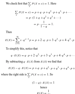
We check first thatP
x
P.X =x/=1:Here
P
x
P.X =x/= p+q·p+q2·p+q3·p+ · · ·
= p·.1+q+q2+q3+ · · ·/
= p· 1
1−q =1: Then
E.X/= ∞ X
x=1
x·qx−1p= p+2·q·p+3·q2·p+4·q3·p+ · · ·:
To simplify this, notice that
q·E.X/=q·p+2·q2·p+3·q3·p+4·q4·p+ · · ·: By subtracting q·E.X/from E.X/we find that
E.X/−q·E.X/= p+q·p+q2·p+q3·p+q4·p+ · · · where the right side isP
x
P.X =x/=1:So
.1−q/·E.X/=1 hence E.X/= 1
p:
The reader is cautioned that the “trick” for summing the series is valid only because the series is absolutely convergent. E.X/could also be found by integrating, with respect to q;the series for E.X/term by term.
With a fair coin, then, since p = 12;an average of two tosses is nec-essary to find the first occurrence of a head. Since P.X =x/ involves a geometric series, X here, as in Example 2.1.6, is often called a geometric random variable.
Mean values generally show a central value for the random variable. Now we turn to a discussion of the dispersion, or variability, of the random
variable. b
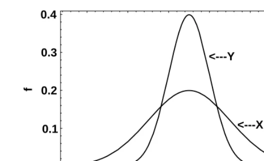
[image:17.612.161.463.53.432.2]2.3.2 Variance of a Random Variable
-2 0 2 4 6 8 0
0.1 0.2 0.3 0.4
f
<---Y
<---X
Figure 2 . 8 Two random variables with mean value 3.
probability distributions, we would no doubt choose Y since the values of Y are less disperse and generally closer to¼than those for X.
There are many ways to measure the fact that Y is less disperse than X. We could look at the range (the largest possible value minus the smallest possible value). Another possibility is to calculate the deviation of each value of X from¼and then calculate the average value of these deviations from the mean, E.X−¼/. This, however, is 0 for any random variable and hence carries absolutely no information whatsoever regarding X:Here is a demonstration that this is so.
E.X−¼/=P
x
.x−¼/·P.X =x/
=P
x
x·P.X =x/−¼·P
x
P.X=x/
=¼−¼=0:
So the positive deviations from the mean exactly compensate for the negative deviations.
One way to avoid this is to consider the mean deviation, E|X−¼|;but this is not commonly done. Yet another way to prevent the positive deviations from compensating for the negative deviations is to square each value of X−¼and then sum the result. This is the usual solution; we call the result the variance, denoted by¦2;which we define as
Definition: ¦2= V ar.X/=E.X−¼/2
so (2.1)
¦2=X
x
.x−¼/2·P.X =x/;
[image:18.612.178.442.56.217.2]2.3 Expected Values of Discrete Random Variables 93
The quantity¦2is then a weighted average of the squared deviations of the values of X from its mean value. The variance may appear to be much more complex than the range or mean deviation. This is true, but the variance also has remarkable properties that we cannot describe now and that do not hold for the range or for the mean deviation. We will consider some of the properties of the variance subsequently.
Ex ample 2.3.2.1
Consider the random variable X with probability distribution function
f.x/= 8 > < > : 1
2 if x =1 1
3 if x =2 1
6 if x =3: Here
E.X/=¼=1·1 2 +2·
1 3 +3·
1 6 =
5 3; so
E.X−¼/2=¦2=
1−5 3
2
·1
2 +
2−5 3
2
·1
3 +
3− 5 3
2
·1
6 = 5 9: b
Before turning to some more examples, we show another formula for ¦2: This formula is often very useful.
Expand Formula 2.1 as follows:
¦2=X
x
.x−¼/2· P.X=x/
=X
x
.x−¼/2· f.x/
=X
x
.x2−2¼x+¼2/· f.x/
=X
x
x2· f.x/−2¼X
x
x· f.x/+¼2
becauseP
x
f.x/=1:NowP
x
x· f.x/=¼, so
¦2 =X
x
x2· f.x/−¼2
so (2.2)
Formula 2.2 is often easier to use for computational purposes than formula 2.1. ¦ is called the standard deviation of X:
Ex ample 2.3.2.2
Refer again to throwing a single die, as in Examples 2.1.1 and 2.3.1.2. We calculate
E.X2/=12·1 6 +2
2
·16 +32·1 6 +4
2
·16 +52·1 6+6
2
·16 = 916
so that ¦2 = 91
6 −. 7 2/
2
= 35
12:
b
Ex ample 2.3.2.3
What is the variance of the geometric random variable whose probability distribution function is P.X =x/=qx−1·p; x =1;2;3; : : :?
Starting with¦2 = E.X2/−¼2, since we know that¼= 1p, we only need to compute E.X2/.
E.X/2 = ∞ X
x=1
x2qx−1p = p.12+22q+32q2+ · · ·/;
from which no easily seen pattern emerges.
Another thought is to consider E[ X.X−1/]. If we write
E[ X.X−1/]= ∞ X
x=1
.x2−x/·P.X =x/
we see that
E[ X.X−1/]= P∞
x=1
x2·P.X =x/− P∞
x=1
x ·P.X =x/ or
E.X2−X/= E.X2/−E.X/:
So if we know E[X.X−1/] we can find E.X2/ and hence calcu-late¦2:In this example, a trick will help as it did in determining E.X/:
2.3 Expected Values of Discrete Random Variables 95
so, multiplying through by q, we have
q·E[X.X−1/]=2·1·q2·p+3·2·q3·p+4·3·q4·p+ · · ·. Subtract the second series from the first and, because p=1−q; it follows that
p·E[ X.X −1/]=2·q·p+4·q2·p+6·q3·p+ · · ·
=2q.1 p+2q p+3q2p+ · · ·/ so
p·E[X.X−1/]=2q·E.X/= 2q p : So
E[ X.X−1/]= 2q p2; and
E.X2/= 2q p2 +
1 p; giving ¦2 = 2q
p2 + 1 p −
1 p2 =
q p2:
b
The value of the variance is quite difficult to interpret at this point, but, as we proceed, we will find more and more uses for the variance. Patience is requested of the reader now, with the promise that these calculations are in fact useful and meaningful. We pause to consider the question, “Does ¦ measure variability?” We can show a general result, albeit a very crude one, in the following inequality.
2.3.3 Tcheby cheff’s Inequality
THEOREM: Suppose the random variable X has mean¼and standard deviation¦. Choose a positive quantity, k. Then
P.| X−¼|≤k·¦ /≥1− 1 k2:
j
Before offering a proof, we consider some special cases. If k=2, the inequality is
P.| X−¼|≤2·¦ /≥1− 1 22 =
3 4;
so 34 of any probability distribution lies within two standard deviations – that is, 2¦– units of the mean while, if k=3, the inequality states that
P.| X−¼|≤3·¦ /≥1− 1 32 =
8 9;
showing that89of any probability distribution lies within 3¦ units of the mean. We will see later that if the specific distribution is known, these inequalities can be sharpened considerably. Now we show a proof.
PROOF: Let P.X=x/= f.x/:Consider two sets of points,
A= {x||x−¼|≥k·¦}
and
B= {x ||x−¼|<k·¦}:
We could then write the variance as
¦2 = X
x∈A
.x−¼/2· f.x/+X
x∈B
.x−¼/2· f.x/:
Now for every point x in A, replace|x−¼|by k·¦, and in B, replace|x−¼| by 0. The crudity of the result is now evident! So
¦2≥ X
x∈A
.k·¦ /2f.x/+X
x∈B
02· f.x/:
Since
X
x∈A
f.x/= P.A/
= P.|X−¼|≥k·¦ /; ¦2≥k2·¦2·P.| X−¼|≥k·¦ /;
from which we conclude that
P.|X−¼|≥k·¦ /≤ 1 k2 or
P.|X−¼|≤k·¦ /≥1− 1 k2:
2.3 Expected Values of Discrete Random Variables 97
While the theorem is far from precise, it does verify that as we move farther away from the mean, in terms of standard deviations, the more of the probability distribution we cover; hence¦ is indeed a measure of variability.
Exercises 2.3
1. A small manufacturing firm sells 1 machine per month with probability 0.3; it sells 2 machines per month with probability 0.1; it never sells more than 2 machines per month. If X represents the number of machines sold per month,
a. find the mean and variance of X.
b. If the monthly profit is 2 X2+3X+1 (in thousands of dollars), find the expected monthly profit.
2. Bolts are packaged in boxes so that the mean number of bolts per box is 100 with standard deviation 3. Use Tchebycheff’s Inequality to find a bound on the probability that the box has between 95 and 105 bolts.
3. Graduates of a distinguished undergraduate mathematics program received gradu-ate school fellowships as follows: 20% received $10,000, 10% received $12,000, 30% received $14,000, 30% received $13,000, 5% received $15,000, and 5% received $17,000.
Find the mean and the variance of the value of a graduate fellowship.
4. A fair coin is tossed 4 times; let X denote the number of heads that occur. Find the mean and variance of X.
5. A batch of 15 electric motors contains 3 defective ones. An inspector chooses 3 (without replacement). Find the mean and variance of X, the number of defective motors in the sample.
6. A coin, loaded to show heads with probability 23, is tossed until a head appears or until 5 tosses have been made. Let X denote the number of tosses made. Find the mean and variance of X.
7. Suppose X is a discrete uniform random variable so that f.x/= n1; x =1;2;3; : : : ;n:Find the mean and variance of X.
8. In exercise 5, suppose the batch of motors is accepted if no more than one defective motor is in the sample. If each motor costs $100 to manufacture, how much should the manufacturer charge for each motor in order to make the expected profit for the batch be $200?
substance. Approximate the probability that a particular one of the measurements is within 5¦=4 units of¼:
10. A manufacturer ships parts in lots of 1000 and makes a profit of $50 per lot sold. The purchaser, however, subjects the product to a sampling inspection plan as follows: 10 parts are selected at random. If none of these parts is defective, the lot is purchased; if one part is defective, the manufacturer returns $10 to the buyer; if 2 or more parts are found to be defective, the entire lot is returned at a net loss of $25 to the manufacturer. What is the manufacturer’s expected profit if 10% of the parts are defective? (Assume that the sampling is done with replacement.)
11. In a lot of 6 batteries, one is worn out. A technician tests the batteries one at a time until the worn-out battery is found. Tested batteries are put aside, but after every third test the tester takes a break and another worker, unaware of the test, returns one of the tested batteries to the set of batteries not yet tested.
a. Find the probability distribution for X, the number of tests required to identify the worn-out battery.
b. Assume the first test of each set of 3 tests costs $5 and that each of the next 2 tests in each set of three tests costs $2. Find the increase in the expected cost of locating the worn-out battery due to the unaware worker.
12. A carnival game consists of hitting a lever with a sledge hammer to propel a weight upward toward a bell. Because the hammer is quite heavy, the chance of ringing the bell declines with the number of attempts; in particular, the probability of ringing the bell on the ith attempt is34i. For a fee, the carnival sells you the privilege of swinging the hammer until the bell rings or until you have made 3 attempts, whichever occurs first.
a. Find the probability distribution of X, the number of hits taken.
b. The prize for ringing the bell on the ith try is $.4−i/, i =1;2;3. How much should the carnival charge for playing the game if it wants an expected profit of $1 per customer?
13. Suppose X is a random variable defined on the points x = 0, 1, 2, 3,: : :Calculate ∞
X
x=0
P.X>x/:
There are many very important specific discrete probability distribution functions that arise in practical applications. Having established some general properties, we now turn to discussions of several of the most important of these distributions.
2.4 Binomial Distribution 99
2.4
c
Binomial Distribution
Among all discrete probability distribution functions, the most commonly occurring one, arising in a great variety of applications, is called the binomial probability distri-bution function.
Consider an experiment where, on each trial of the experiment, one of only two outcomes occurs, which we describe as success, (S) or failure, ( F). For example, a manufactured part is either good or does not meet specifications; a student’s examina-tion score is passing or it is not; a team wins a basketball game or it does not – these are some examples, and the reader can no doubt think of many more. One of these outcomes can be associated with success and the other with failure; it does not matter which is which.
In addition to the restriction that there be two and only two outcomes on each trial of the experiment, suppose further that the trials are independent, and that the probabilities of success or failure at each trial remain constant from trial to trial and do not change with subsequent performances of the experiment.
The individual trials of such an experiment are often called Bernoulli trials. Consider, as a specific example, five independent trials with probability 23 of success at any trial. Then, if interest centers on the occurrence of exactly three successes, we note that exactly three successes can occur in ten different ways:
S S S F F;S S F S F;S F S S F;F S S S F;S F S F S; S S F F S;F S S F S;S F F S S;F S F S S;F F S S S:
There are 53Ð
=10 of these mutually exclusive orders. Each has probability
2 3
3 ·
1 3
2
, so
P.exactly 3 S′s in 5 trials)=
5 3
·
2 3
3 ·
1 3
2 = 80
243:
Now return to the general situation. Let the probabilities be P.S/= p and P.F/=q=1−p, and let the random variable X denote the number of successes in n trials of the experiment. Any specific sequence of exactly x successes and n−x failures has probability px·qn−x:The successes in such a sequence can occur at nxÐ positions so, since the sequences are mutually exclusive,
P.X=x/=
n x
px·qn−x; x =0;1;2; : : : ;n; (2.3)
giving the probability distribution function for a binomial random variable.
Now does Formula 2.3 define a probability distribution? Since P.X=x/≥0 and
n
X
x=0
P.X=x/=
n
X
x=0
n x
px·qn−x =.q+p/n =1
by the binomial theorem, we conclude that Formula 2.3 defines a probability distri-bution.
It is interesting to note that individual terms in the binomial expansion of.q+p/n, if p+q=1;represent binomial probabilities.
Ex ample 2.4.1
A student has no knowledge whatsoever of the material to be tested on a true-false examination, and so the student flips a fair coin in order to determine the response to each question. What is the probability that the student scores at least 60% on a ten-item examination?
Here the binomial variable, X, the number of correct responses, has n=10;and p=q = 12. We need
P.X ≥6/= 10 X
x=6
10 x
1 2
x
1 2
10−x
:
Now we find that P.X ≥6/= 193512 =0:376953.
These calculations can easily be done with a pocket computer. If we want to investigate the probability that at least 60% of the questions are answered correctly as the number of items on the examination increases, then use of a computer algebra system is recommended for aiding in the calculation. Many computer algebra systems contain the binomial proba-bility distribution as a defined probaproba-bility distribution; for other systems, the probability distribution function may be entered directly. The following results can be found where n is the number of trials and P is the probability of at least 60% correct:
n 10 40 80 100
P 0.376953 0.134094 0.0464559 0.028444
Clearly, guessing is not a sensible strategy on a test with a large number
of items. b
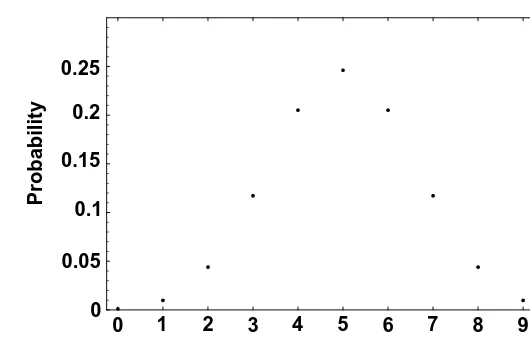
Ex ample 2.4.2
Graphs of P.X =x/= nxÐ
2.4 Binomial Distribution 101
n =100 with p = 12 in each case. We see that each curve is bell-shaped or normal-like, and the distributions are symmetric about x =5 and x=50; respectively.
0 1 2 3 4 5 6 7 8 9 10
X 0
0.05 0.1 0.15 0.2 0.25
Probability
Binomial distribution, n=10;p=1=2:
34 37 40 43 46 49 52 55 58 61 64 X
0 0.02 0.04 0.06 0.08
Probability
Figure 2 . 9 Binomial distribution,n=100, p=1=2:
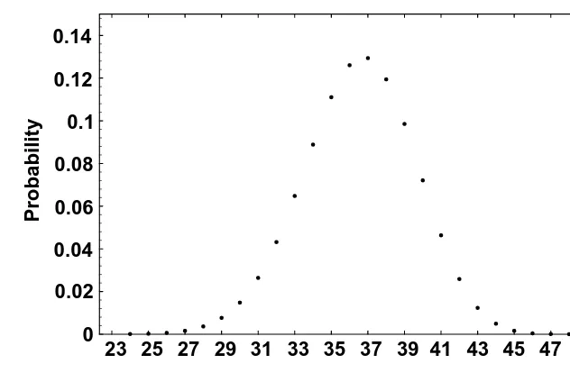
[image:27.612.186.451.103.272.2]23 25 27 29 31 33 35 37 39 41 43 45 47 49 X
0 0.02 0.04 0.06 0.08 0.1 0.12 0.14
Probability
Figure 2 . 1 0 Binomial distribution,n=50, p=3 4.
We will discuss the reason for the normal appearance of the binomial distribution in the next chapter. Appendix 1 contains a procedure for select-ing a sample from a binomial distribution and for simulatselect-ing an experiment consisting of flipping a loaded coin. b
2.5
c
A Recursion
If a computer algebra system is not available, calculating values of P.X =x/ = nx
Ð
px·qn−x can certainly become difficult, especially for large values of n and small values of p. In any event, nxÐ
becomes large while px·qn−xbecomes small. By calculating the ratio of successive terms we find an interesting result, which will aid in making these calculations (and which has other interesting consequences as well).
P.X=x/ P.X =x−1/ =
n x
px·qn−x
n x−1
px−1·qn−x+1
;x =1;2; : : : ;n
This can be simplified to
P.X=x/ P.X =x−1/ =
n−x+1 x ·
[image:28.612.149.465.57.269.2]2.5 A Recursion 103
P.X=x/= n−x+1
x · p
q · P.X=x−1/ ;x=1;2; : : : ;n: (2.4)
Formula 2.4 is another example of a recursion since it expresses one value of a function, here P.X =x/, in terms of another value of the function, here P.X =x−1/: Given a starting point and the recursion, any value of the function can be computed. In this case, since n failures has probability qn; P.X =0/=qn is a natural starting value. We then find that
P.X=0/=qn; so
P.X=1/=n· p
q ·P.X=0/=n· p q ·q
n
=
n 1
· p·qn−1; so
P.X=2/= .n−1/
2 ·
p
q ·P.X=1/=
.n−1/
2 ·
p
q ·n· p·q
n−1
=
n 2
·p2·qn−2
and so on, giving the expected result that P.X=x/= nx
Ð
px·qn−x;x=0;1; : : : ;n: So we can recover the probability distribution function from the recursion.
Recursions can be easily programmed, and recursions such as Formula 2.4 are also of some interest for theoretical purposes. For example, consider locating the maximum, or most frequently occurring value, of P.X =x/.
If we require that P.X =x/≥ P.X=x−1/then, from Formula 2.4,
n−x+1 x ·
p q ≥1:
This reduces to x ≤ p·.n+1/, so we can conclude that the value of X with the maximum probability is X= ⌊p·.n+1/⌋where⌊x⌋denotes the largest integer in x.
2.5.1 The Mean and Variance of the Binomial
The recursion 2.4 can be used to determine the mean and variance of a binomial random variable.
Consider first¼=
n
P
x=0
x· P.X=x/. Recursion 2.4 is
P.X=x/= n−x+1 x ·
p
Multiplying through by x and summing from 1 to n gives
n
P
x=1
x·P.X =x/=
n
P
x=1
[n−.x−1/]· p
q · P.X=x−1/; so
¼= p
q ·n·[1−P.X=n/]− p q ·
n
P
x=1
.x−1/· P.X=x−1/;
or
¼= p
q ·n·.1− p
n/
− p
q ·[¼−n· P.X=n/]; which reduces to
¼=n·p:
This result makes a good deal of intuitive sense: if we toss a coin, loaded to come up heads with probability 34, 1000 times, we expect 1000· 34 =750 heads. So in n trials of a binomial experiment with p as the probability of success, we expect n· p successes.
The variance can also be found using Formula 2.4. We first calculate E.X2/:
E.X2/=
n
X
x=1
x2·P.X=x/=
n
X
x=1
x·[n−.x−1/]· p
q ·P.X =x−1/
=n· p q ·
n
X
x=1
[.x−1/+1]·P.X= x−1/− p q ·
n
X
x=1
x·.x−1/·P.X =x−1/
Then, because
n
P
x=1
.x−1/·P.X =x−1/=¼−n·P.X=n/
and since
n
P
x=1
x·.x−1/·P.X=x−1/=
n
P
x=1
[.x−1/2+.x−1/]· P.X=x−1/;
it follows that
E.X2/= p·.n−1/·.np−npn/+n·p·.1− pn/+n2· pn+1;
and this reduces to E.X2/=np2.n−1/+np:Therefore,
2.5 A Recursion 105 Ex ample 2.5.1.1
We apply the above results to a binomial experiment in which p =q = 12 and n =100 trials. Here E.X/=¼=n·p=50 and ¦2=npq =25. Tchebycheff’s Inequality with k =3 then gives
P[n·p−k·√n·p·q ≤ X ≤n·p+k·√n·p·q]≥1− 1 k2 so
P[50−3·5≤ X ≤50+3·5]≥ 8 9 or
P[35≤ X ≤65]≥ 8 9 . But we find exactly that
65 X
x=35
100 x
·
1 2
100
=0:99821;
verifying Tchebycheff’s Inequality in this case. b
Exercises 2.5
1. A test is conducted to determine the concentration of a chemical in a lawn weed killer that will effectively kill dandelions. It is found that a given concentration of the chemical will kill, on average, 80% of the dandelions in 24 hours. A test is performed on 20 dandelions. Find the probability that
a. exactly 14 are killed in 24 hours. b. at least 10 are killed in 24 hours.
2. A fair die is rolled 240 times. Find the probability that the number of twos or threes is between 75 and 83, inclusive.
3. A manufacturer of dry cells makes 2 types of batteries that appear to be identical. Batteries of type A last more than 600 hours with probability 0.30, and batteries of type B last more than 600 hours with probability 0.40.
a. What is the probability that 5 out of 10 of the type A batteries last more than 600 hours?
b. Of 50 type B batteries, how many are expected to last at least 600 hours? c. What is the probability that 3 type A batteries have more batteries lasting 600
4. X and Y play the following game: X tosses 2 fair coins and Y tosses 3. The player throwing the greater number of heads wins. In case of a tie, the throws are repeated until a winner is determined.
a. What is the probability that X wins on the first play? b. What is the probability that X wins the game?
5. In a political race it is known that 40% of the voters favor candidate C. In a random sample of 100 voters, what is the probability that
a. between 30 and 45 voters favor C? b. exactly 36 voters favor C?
6. A gambling game is played as follows. A player, who pays $4 to play the game, tosses a fair coin 5 times. The player wins as many dollars as heads are tossed.
a. Find the probability distribution for N , the player’s net winnings. b. Find the mean and variance of the player’s net winnings.
7. A red die is fair, and a green die is loaded so that the probability it comes up 6 is 101 .
a. What is the probability of rolling exactly 3 sixes in 3 rolls with the red die? b. What is the probability of at least 30 sixes in 100 rolls of the red die? c. The green die is thrown 5 times and the red die is thrown 4 times. Find the
probability that a total of 3 sixes occurs.
8. What is the probability of one head twice in 3 tosses of 4 fair coins?
9. A commuter’s drive to work includes 7 stoplights. Assume the probability that a light is red when the commuter reaches it is 0.20, and that the lights are far enough apart to operate independently.
a. If X is the number of red lights the commuter stops for, find the probability distribution function for X.
b. Find P.X ≥5/:
c. Find P.X ≥5|X ≥3/:
10. The probability of being able to log on a computer system from a remote terminal during a busy period is 0.7. Suppose that 10 independent attempts are made and that X denotes the number of successful attempts.
a. Write an expression for the probability distribution function, f.x/. b. Find P.X ≥5/:
2.5 A Recursion 107
11. An experimental rocket is launched 5 times. The probability of a successful launch is 0.9. Let X denote the number of successful launches. A study has shown that the net cost of the experiment, in thousands of dollars, is 2−3X2. Find the expected net cost of the experiment.
12. Twenty percent of the IC chips made in a plant are defective. Assume that a binomial model is appropriate.
a. Find the probability that, at most, 13 defective chips occur in a sample of 100. b. Find the probability that 2 samples, each of size 100, will have a total of exactly
26 defective chips.
13. A coin, loaded to come up heads with probability 23, is tossed 5 times. If the number of heads is odd, the player is paid $5. If the number of heads is 2 or 4 the player wins nothing; if no heads occur, the player tosses the coin 5 more times and wins, in dollars, the number of heads thrown. If the game costs $3 to play, find the probability distribution of N , the player’s net winnings.
14. a. Show that the probability of being dealt a full house (3 cards of one value and 2 of another value) in poker is about 0.0014.
b. Find the probability that in 1000 hands of poker you will be dealt at least 2 full houses.
15. An airline knows that 10% of the people holding reservations on a given flight will not appear. The plane holds 90 people.
a. If 95 reservations have been sold, find the probability that the airline will be able to accommodate everyone appearing for the flight.
b. How many reservations should be sold so that the airline can accommodate everyone who appears for the flight 99% of the time?
16. The probability that an individual seed of a certain type will germinate is 0.9. A nurseryman sells flats of this type of plant and wants to “guarantee” (with probability 0.99) that at least 100 plants in the flat will germinate. How many plants should he put in each flat?
17. A coin with P.H/= 12is flipped 4 times and then a coin with P.H/= 23 is tossed twice. What is the probability that a total of 5 heads occurs?
18. a. Each of 2 persons tosses 3 fair coins. What is the probability each gets the same number of heads?
b. In part a, what is the probability that X1+X2is odd, where X1is the number of heads the first person tosses and X2 is the number of heads the second person tosses?
19. Find the probability that more than 520 heads occur in 1000 tosses of a fair coin.
20. How many times must a fair coin be tossed if the probability of obtaining at least 40 heads is at least 0.95?
21. Samples of 100 are selected each hour from an assembly line that produces items, 20% of which are defective.
a. What is the probability that at most 15 defectives are found in an hour? b. What is the probability that a total of 47 defectives is found in the first 2 hours?
22. A small engineering college would like to have an entering class of 360 students. Past data indicates that 85% of those accepted actually enroll in the class. How many students should be accepted if the probability the class will be at least 360 is to be approximately 0.95?
23. A fair coin is tossed repeatedly. What is the probability that the number of heads tossed reaches 6 before the number of tails tossed reaches 4?
24. Evaluate the sums
n
X
x=0 x·
n x
px·qn−xand
n
X
x=0
x·.x−1/·
n x
px·qn−x
directly and use these to verify the formulas for¼and¦2 for the binomial distri-bution.
[Note that
n
X
x=0
n
x
· px·.1− p/n−x =[ p+.1− p/]n =1:]
25. In exercise 4, show that the game is fair if X wins if he tosses at least as many heads as Y .
2.6
c
Some Statistical Considerations
We pause here and in the next two sections to show some statistical applications of the probability theory we have developed so far. From time to time in this book we will show some applications of probability theory to statistics and the statistical analysis of data as well as to other applied situations; this is our first consideration of statistical problems.
2.6 Some Statistical Considerations 109
this would be a number of good items from the process, say X, and we would surely use X in some way to estimate p. How precisely can we use X to estimate p?
It would appear natural to estimate p by the proportion of good items in the sample,
X
n:Since X is a random variable, so is X
n:We can calculate the expected value of this
random variable as follows:
E
X n
½ =
n
P
x=0 x
n ·P.X =x/= 1 n·
n
P
x=0
x·P.X=x/;
so
E
X n
½ = 1
n ·n· p= p:
This indicates that, on average, our estimate for p gives the true value, p. We say that our estimator, Xn, is an unbiased estimator for p.
This gives us a way of estimating p by a single value. This single value is dependent upon the sample, and if we choose another sample, we are likely to find another value of X, and hence arrive at another estimate of p. Could we also find a “likely” range for the value of p?
To answer this, consider a related question. If we have a binomial situation with probability p and sample size n, what is a likely range for the observed values of the random variable, X? The answer of course depends upon the meaning of the word likely. Suppose that a likely range for the values of a random variable is a range in which the values of the variable occur with probability 0.95.
With the considerable aid of our computer algebra system, we can evaluate a number of different binomial distributions. We vary n; the number of observations, and p;the probability of success. In each case we find the proportion of the values of X that lie within two standard deviations of the mean; that is, the proportion of the values of X that lie in the interval¼±2¦ =n· p±2√n· p·.1−p/:We select the constant two because we need to find a range that includes a large portion – 95% – of the values of X, and two appears to be a reasonable multiplier for the standard deviation. Table 2.6.1 shows the results of these calculations. Here P represents the probability that an observed value of the random variable X lies in the interval¼±2¦ =n· p±2√n·p·.1− p/: The values of n and p have been chosen so that the end-points of the intervals are integers.
We are led to believe from the table, regardless of the value of p, that at least 95% of the values of the variable X lie in the interval¼±2¦:(Later we will show, for large values of n, regardless of the value of p, that the probability is approximately 0:9545, a result supported by our calculations.) So we have
P.¼−2¦ ≤ X≤¼+2¦ /≥0:95: (2.5)
Solving the inequalities for¼, we have
TABLE 2.6.1
n p ¦ ¼±2¦ P
36 12 3 12,24 0.971183
64 12 4 24,40 0.967234
100 12 5 40,60 0.964800
144 12 6 60,84 0.963148
196 12 7 84,112 0.961530
18 13 2 2,10 0.978800
72 13 4 16,32 0.967288
162 13 6 42,66 0.963177
288 13 8 80,112 0.961066
48 14 3 6,18 0.971345
192 14 6 36,60 0.963214
432 14 9 90,126 0.960373
10000 12 50 4900,5100 0.954494
11250 13 50 3650,3850 0.954497
13872 14 51 3366,3570 0.954499
Replacing¼and¦ by n·p and√n·p·q, respectively, Formula 2.6 becomes
P.X−2√n· p·q ≤n·p≤ X+2√n· p·q/≥0:95: (2.7)
The inequalities in Formula 2.7 can now be solved for p. The result is
P n X+2n−2
p
n2X+n2−n X2 n2+4n ≤ p≤
n X+2n+2pn2X+n2−n X2 n2+4n
!
≥0:95: (2.8)
Our thinking here is as follows: If we find an interval that contains at least 95% of the values of X and if p is unknown, then those same values of X will produce an interval in which p;in some sense, is likely to lie. The end points produced by Formula 2.8 comprise what we call a 95% confidence interval for p:
While Formula 2.5 gives a likely range of values of X if p is known, Formula 2.8 gives a likely range of values of p if X is known. So we have a response to a variant of our first question: If X successes are observed in n binomial trials, what is a likely value for p?
2.6 Some Statistical Considerations 111
probability statement! Why not? The reason is that p is an unknown constant. It either lies in the stated interval or it doesn’t. Then what does the 95% mean?
Here’s a way of looking at this. Consider samples of