On the empirical construction of implications between
bi-valued test items
* Martin Schrepp
Schwetzinger straße86, 68766 Hockenheim, Germany
Abstract
We describe a data-analytic method which allows one to derive implications between test items from observed response patterns to these items. This method is a further development of item tree analysis (J.F.J.v. Leeuwe, Nederlands Tijdschrift voor de Psychologie, 29 (1974) 475–484). A simulation study shows that the improvements have a positive effect on the ability of the method to reconstruct the valid implications from data. The improved method is able to reconstruct the underlying structure on the items with high accuracy. As a concrete example the implications in a set of letter series completion problems are analysed. 1999 Elsevier Science B.V. All rights reserved.
Keywords: Item tree analysis; Test items; Improved method
1. Introduction
We deal with the question of how a structure on an item set can be derived from observed response patterns to these items. Assume that we have a binary item set I, i.e. a set of n items to which every subject may respond positive (1) or negative (0). We try to derive the logical implications between the items from the observed data.
Assume, for example, that I is a problem set. In this case a subject can either solve (1) a problem or fail (0) in solving the problem. In this example an implication j→i can be
interpreted as ‘every subject who is able to solve j is also able to solve i’.
As a second example assume that I is a set of statements from a questionnaire to which subjects can either agree (1) or disagree (0). In this case an implication j→i can
be interpreted as ‘every subject who agrees to statement j also agrees to statement i’. Because of our interpretation of→ as a logical implication, the set of implications on
*Tel.: 149-6205-189-696.
E-mail address: [email protected] (M. Schrepp)
I should form a reflexive and transitive relation on I. We call such a relation in
accordance with Doignon and Falmagne (1985) a surmise relation on I.
There are a number of data-analytic techniques which try to derive such logical implications between items from binary datasets. See, for example, Leeuwe (1974), Flament (1976), Buggenhaut and Degreef (1987), Duquenne (1987), and Theuns (1994). There are some obvious connections between these data-analytic techniques and the theory of knowledge spaces (Doignon and Falmagne, 1985). In this approach a knowledge domain is represented as a finite set I of questions. The subset of questions from I that a subject is capable of solving is called the knowledge state of that subject. In general, not every subset of I will be a possible knowledge state of a subject. Thus, the set of possible knowledge states, which is called the knowledge structure, will be a proper subset of the power set of I. This can be used for an efficient adaptive diagnosis of students knowledge (see Falmagne and Doignon, 1988).
A data-analytic technique which derives the set of valid logical implications from observed response patterns determines a knowledge structure on the item set. This knowledge structure consists of all subsets A of I which are consistent with the derived implications, i.e. which fulfil the condition ( j→i )∧( j[A)⇒i[A for all i, j[I (for
details see Doignon and Falmagne, 1985).
2. Problems in reconstructing implications from data
Let I5hi , . . . , i1 nj be an item set. Assume that R is a set of m binary response patterns to I. R contains for each subject who responded to the items in I a response
pattern r. Such a response pattern r can be considered as a mapping r: I→h0, 1j. Our goal is to derive all valid implications j→i from this dataset R.
We assume that the dataset R contains all relevant patterns. If many patterns occurring in the population are not contained in R, for example because of a bad sampling, we cannot hope to derive the valid implications from this dataset.
Assume that there is an implication j→i between two items i, j[I. In this case r( j )51 should imply r(i )51 for every response pattern r[R.
A direct approach to derive the implications from the data is to accept j→i if there is
no response pattern r[R with r(i )50 and r( j )51. We call such a response pattern r a
counterexample for the implication j→i. Such a direct approach is clearly insufficient,
since some of the response patterns may be influenced by random errors.
We have to consider two different error types. Assume that t is the ‘true’ state of a subject, i.e. the response pattern of the subject under ideal conditions where no errors occur. Let r be the observed response pattern of the subject. We define the conditional probabilities a and b by:
a: probability that r(i )50, given t(i )51,
If, for example, I is a set of problems, thena is the probability of a careless error andb
is the probability of a lucky guess.
A method which tries to derive the valid implications from data has to deal with the influence of random errors in the data. Therefore, an implication may be accepted even if a small number of counterexamples for this implication are observed.
3. Item tree analysis (ITA)
We describe in the following a data-analytic method which was proposed by Bart and Krus (1973) and further developed by Leeuwe (1974). The central idea of this method is to detect an ‘optimal’ tolerance level Lopt and to accept all implications for which no more than Lopt counterexamples are observed.
3.1. The algorithm
We describe the algorithm of ITA with the symbols from Leeuwe (1974), where an implication j→i is written as i#j.
We define for items i, j[I:
bij[uhr[Rur(i )50∧r( j )51ju.
The value bij is the number of counterexamples for j→i in the dataset R. Every
tolerance level L50, . . . , m defines a binary relation #L by:
i#Lj:⇔bij#L.
According to our interpretation of #L this relation should be transitive, i.e. i#Lj and j#Lk should imply i#Lk. Leeuwe (1974) showed that #0 is transitive, but that transitivity can be violated for L.0.
Since a relation #L is constructed for every tolerance level L the problem arises of how to determine the most adequate tolerance level Lopt.
A simple measure for the fit between a binary relation# on an item set I and a set R of observed response patterns to the items in I is the reproducibility coefficient Repro(#, R).
Let W(#) be the set of all possible response patterns which are consistent with #. This set is defined by:
W(#)[hw: I→h0, 1ju;i, j (i#j∧w( j )51→w(i )51)j.
In the terminology of knowledge space theory (Doignon and Falmagne, 1985) the set
W(#) is called the quasi-ordinal knowledge space corresponding to the relation #. Note that W(#L)#W(#L9) for L9 #L. Thus, the higher the tolerance level L is, the
lower is the number of response patterns consistent with #L. Define for w[W(#) and r[R the distance d(r,w) by:
The distance between w and r is the number of items i for which w(i ) and r(i ) have different values.
We define now the reproducibility coefficient (Guttman, 1944) by:
min(hd(r, w)uw[W(#)j)
]]]]]]]
Repro(#, R)[12
O
uRu uIu
r[R
Repro(#, R) is the proportion of cells in the data matrix which are consistent with #. The higher Repro(#, R) is, the better is the fit between#and R. Notice that Repro(#,
R) is a direct generalization of the reproducibility coefficient of a Guttman-Scale.
Repro(#, R) is a useful measure to evaluate the ability of a binary relation to explain
a set of response patterns. But Repro(#, R) cannot be used to determine the best
relation #L.
Consider two tolerance levels L, L9 with L9 #L. This implies W(#L)#W(#L9). Thus, min(hd(r, w)uw[W(#L9)j)#min(hd(r, w)uw[W(#L)j) for each r[R. This
directly shows Repro(#L9, R)$Repro(#L, R), i.e. Repro(#L, R) decreases with an increasing tolerance level L. Note that Repro(#0, R)51.
Therefore, Leeuwe (1974) introduced a different method to evaluate the adequacy of a relation #L.
The fit between #L and the dataset R is evaluated by a comparison of the observed correlations between items with the expected correlations if it is assumed that #L is the correct relation. The fit between the dataset R and #L is measured by the correlation
agreement coefficient (Leeuwe, 1974) which is defined by:
2 2
]]] *
CA(#L)[12n(n21)
O
(rij2r ) ,ij i,j*
where r is the Pearson’s correlation (phi-coefficient) between item i and item j and rij ij is defined by:
The value p is the relative frequency of subjects who responded positive (1) to item ii and p is the relative frequency of subjects who responded positive to item j.j
The higher the value of CA(#L) is, the better is the fit between the relation #L and the dataset R.
*
Note that we should have rij5rij if #L is the correct relation and j→i is a correct
*
implication. But for item pairs (i, j ) with i¢j and j¢i it is possible that rij.rij50, even if #L is the correct relation and the data are noiseless. This can be illustrated by the following example.
a→c, a→d, and c→d are true. Thus, each subject should show one of the following
Assume that each of these response patterns occurs with the same frequency in the
population and that no errors are possible (a 5 b 50). Then we should have rbd5
* *
0.09.rbd50 and rbc50.167.rbc50.
*
As the example shows, the expected correlation rij can differ from the true correlation
r for non-connected item pairs (i, j ), i.e. items i, jij [I with i¢j and j¢i.
Leeuwe (1974) suggests the following procedure to detect the optimal tolerance level
Lopt. First, a critical value 0#d #1 for the reproducibility coefficient Repro(#L, R) is set. Second, for this critical valued we define the set + by:
d
+ [hL[h0, . . . , mjuRepro(# , R)$d∧# is transitivej.
d L L
The set + consists of all tolerance levels L for which # is transitive and the
d L
reproducibility coefficient Repro(#L, R) is higher than the critical value d. Note that
+ ±5, since # is always transitive and Repro(# , R)51. Third, the level L[+
d 0 0 d
for which CA(#L) shows the highest value is chosen as the optimal tolerance level Lopt. This strategy to derive the optimal tolerance level Lopt and the best surmise relation
#Lopt is problematical because of two points.
First, a single intransitivity in #L results in excluding the whole relation #L from the process which searches for the best relation. If intransitivities are likely (small number of observed response patterns, high error probabilities) many of the relations
#L will contain intransitivities. The choice of the best fitting relation is in such cases based on a small number of transitive relations #L.
Second, the remaining transitive relations are compared with the correlation
agree-*
ment coefficient. This coefficient is based on a comparison of r and r . As we haveij ij
*
shown in the example it is possible that rij.rij for non-connected item pairs (i, j ). Thus, for relations which contain many non-connected item pairs it seems possible that the correct relation #L will not have the best CA(#L) value.
3.2. A simulation study
The four surmise relations81,82,83and84differ in the number of non-connected item pairs. The relation81 is a linear order (and contains therefore no non-connected pairs), the relation 82 contains three non-connected pairs, the relation 83 contains 11
1
non-connected pairs, and the relation 84 contains 15 non-connected pairs . In each simulation the following steps were repeated m times.
1. A pattern r is chosen randomly from the quasi-ordial knowledge space W(8)
corresponding to 8. 2. For each item i:
• if r(i )51, then r(i ) is changed with probability a to 0, • if r(i )50, then r(i ) is changed with probability b to 1.
The result of this process is a simulated dataset R(a, b, m). This simulated dataset was analysed with ITA. Let 8ITA be the best solution concerning ITA, i.e. the transitive relation #L with the highest CA-value.
The relation 8ITA is then compared to the true surmise relation 8 by:
D(8,8ITA)5uh(i, j )u(i8j∧iWITAj )∨(i8ITAj∧iWj )ju.
D(8, 8ITA) is the number of pairs (i, j ) for which the true dependency (i.e. i8j or iWj ) is not properly reconstructed by ITA.
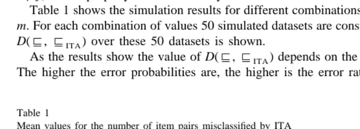
Table 1 shows the simulation results for different combinations of values fora,b and
m. For each combination of values 50 simulated datasets are constructed and the mean of D(8, 8ITA) over these 50 datasets is shown.
As the results show the value of D(8,8ITA) depends on the values fora, b and m. The higher the error probabilities are, the higher is the error rate in reconstructing the
Table 1
Mean values for the number of item pairs misclassified by ITA
a/b 81 82 83 84
m 50 100 200 50 100 200 50 100 200 50 100 200
0.03 / 0.03 2.8 0.5 0.1 3.7 1.9 1 4.4 2.4 1.1 3.9 4.1 2.2
0.03 / 0.05 4 1.7 0.2 5 2.7 1.4 5 3.7 2.5 5.3 4.6 4.1
0.03 / 0.07 6 2.5 0.7 5.9 3.7 2.8 6.5 6 4.2 6.4 5.9 6
0.05 / 0.03 2.9 1.4 0.2 4.7 2.6 1.1 5 3.5 1.6 5.1 3.7 2.5 0.05 / 0.05 4.3 2.9 0.3 5.5 3.9 1.8 5.9 4.8 3.3 5.8 5.3 4.9 0.05 / 0.07 6.8 4.4 0.5 7.3 6 3.8 6.9 6.8 5.9 7.2 6.8 6.6 0.07 / 0.03 4.6 1.9 0.4 5.4 4.2 1.5 5.6 4.3 2.3 5.2 3.9 3.7 0.07 / 0.05 5.8 3.1 0.6 7.1 5.1 3.6 7 6.1 4.2 6.4 6.1 6 0.07 / 0.07 9.1 4.8 1.5 9.2 7.3 5.5 8.4 7.7 7.3 7.9 7.8 8.2
1
correct implications. The more simulated data patterns are available, the better is the ability of ITA to reconstruct the correct implications.
The simulation results are quite different for the four surmise relations. Therefore, the structure of the surmise relation also had an influence on the error rate.
As the results show, the error rate is low if the error probabilitiesa,bare low and the number of non-connected pairs in the surmise relation is low (i.e. if the surmise relation is more or less linear). The error rate increases significantly with the number of non-connected pairs in the surmise relation.
For example, for84anda 5 b 50.07 the error rate is around 8. So in average eight of the 56 possible pairs (i, j ) are misclassified. The error rate does not decrease with m, thus the error is systematical.
4. Improvement of ITA
As a result of the simulation study we modify ITA concerning two points. First, we construct only transitive relations. Second, we change the method of determining the most adequate tolerance level.
4.1. Inductive construction of surmise relations
The idea is to define the relations8L (we use a different symbol to distinguish these
relations from the relations #L constructed in ITA) by an inductive construction
process.
We start this inductive construction process with the transitive relation 80[#0. Assume in the induction step that we have already constructed a transitive relation
8L. Define the set SL11 by:
SL11[h(i, j )ubij#L11∧iWLjj.
The set SL11 consists of all item pairs (i, j )[⁄ 8L which have at least L11 counterexamples in the dataset. The elements of SL11 are the candidates which may be added to 8L in this step of the construction process.
To ensure that the relation8L11 is transitive we must avoid adding pairs (i, j ) from
SL11to8L11which cause an intransitivity to pairs contained in8Lor other pairs added in this step.
A pair (i, j )[SL11is contained in an intransitive triple concerning8L if there exists ( j, k) with bjk#L11∧bik.L11 or (h, i ) with bhi#L11∧bhj.L11. Define
T(8L) as the set of all (i, j )[SL11which are contained in at least one intransitive triple concerning8L.
To ensure the transitivity of8L11 we add only those pairs from SL11 to8L which are not contained in an intransitive triple concerning 8L. Therefore,
It is possible that the set h(i, j )[SL11u(i, j )[⁄ T(8L)j is empty. In this case8L11 and
8L are identical.
The relation 8L11 is transitive, since 8L was assumed to be transitive and the construction makes sure that no intransitive triples can be added in a step of the construction process. If #L11 is transitive, then 8L11 is equal to #L11. The set of surmise relations constructed by this inductive process contains therefore all transitive relations #L. Note that i8Lj implies i#Lj for all i, j[I.
If the item set I is big or if the error probabilitiesa andb are high, then many of the relations #L will be intransitive. In this case the number of different relations8L will be much higher than the number of transitive relations #L. Therefore, the inductive construction process allows us to search for the best fitting relation in a bigger set of transitive relations. This point is discussed also in our practical application in the next section.
4.2. A new method to determine the optimal tolerance level
Assume that 8L is the ‘correct’ surmise relation. How many counterexamples for
j→i should occur under this assumption?
*
We have to distinguish two cases. First, assume iWLj. Then bij should be the
expected value of the number of data patterns r with r(i )50 and r( j )51. This number is given by
*
bij5(12p ) p m,i j
where m is the size uRu of the dataset.
Second, assume i8Lj. Then only violations of j→i through random errors should
*
occur. The expected number of violations bij is in this case given by
*
bij5gLp m,j
*
wheregLis a constant which describes the probability of random errors. Therefore, bij is the number of data patterns in which item j is assigned a 1 (since only in this case a violation can occur) multiplied by a constant which reflects the influence of random errors.
The basic idea is to use the comparison of the observed values b and the expectedij
*
values bij under the assumption that 8L is correct to determine the most adequate
tolerance level.
If we assume that8L is correct, then we are able to estimate the error constantgL by:
O
hb /p mui8 j∧i±jjij j L
]]]]]]]
gL[ ,
(u8Lu2n)
where n is the size of the item set I and m is the number of response patterns in the dataset R. Here b /p m is the number of observed counterexamples to iij j 8Lj relative to
the number of cases in which such a counterexample is possible. The valueu8Lu2n is
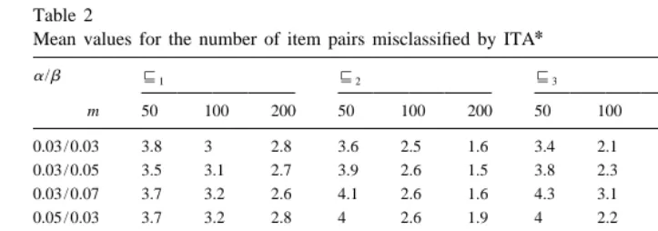
Table 2
*
Mean values for the number of item pairs misclassified by ITA
a/b 81 82 83 84
m 50 100 200 50 100 200 50 100 200 50 100 200
0.03 / 0.03 3.8 3 2.8 3.6 2.5 1.6 3.4 2.1 0.7 2.1 1.2 0.6
0.03 / 0.05 3.5 3.1 2.7 3.9 2.6 1.5 3.8 2.3 1.2 2.8 1.6 1.1
0.03 / 0.07 3.7 3.2 2.6 4.1 2.6 1.6 4.3 3.1 1.9 3 2.2 1.3
0.05 / 0.03 3.7 3.2 2.8 4 2.6 1.9 4 2.2 1.4 2.5 1.2 0.7
0.05 / 0.05 3.7 3.2 2.7 4.4 2.6 1.7 4.1 2.7 1.6 3 1.8 0.8
0.05 / 0.07 3.7 3.1 2.6 4.6 2.8 1.8 4.9 3.1 2.5 3.2 2.3 1.1
0.07 / 0.03 4.5 3.1 2.6 4.2 2.9 2 3.8 2.8 1.5 2.5 1.2 0.5
0.07 / 0.05 4.2 3 2.4 4.8 3.2 1.9 4.3 2.9 1.8 2.8 1.6 0.7
0.07 / 0.07 3.9 3 2.5 5.2 3 2.1 4.8 3.6 2.5 3.2 2.4 1.2
The fit between 8L and the dataset R can now be evaluated by:
2 2
*
diff(8L, R)[
O
(bij2b ) /(nij 2n). i±jThe most adequate surmise relation 8L concerning R is the one with the minimal
diff(8L, R) value.
We call in the following the analysis method based on the inductive construction of
*
surmise relations 8L and on the minimal diff-value ITA .
4.3. Simulation study
The same procedure as described in the simulation study concerning ITA is used. The
*
only difference is that we now use ITA to analyse the simulated dataset R(a,b, m). Let
*
8ITA* be the best solution concerning ITA .
Table 2 shows the simulation results for the different value combinations ofa,b and
m. For each combination of values 50 simulated datasets are generated and the mean of D(8, 8ITA*) over these 50 simulated datasets is shown.
As in the first simulation the value of D(8,8ITA ) depends on the values for a, b
*
and m. The higher the error probabilities are, the higher is the error rate. The more simulated data patterns are available, the lower is the error rate (for fixed values ofa,
b).
As the results show the structure of the underlying surmise relation also had an
* *
*
5. An example for data analysis with ITA and ITA
*
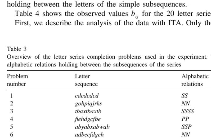
As a practical application of ITA and ITA we analyse a dataset from Schrepp (1995). In this investigation a group of 51 subjects tried to solve 20 letter series completion problems, which are shown in Table 3.
Such letter series completion problems have a simple structure. Given a sequence of letters of the alphabet a subject is required to find a continuation which is in accordance with the rule used to generate the sequence.
The letter sequences commonly used, for example in intelligence tests, are a mixture of simple sequences in which every letter is in a specific relation to its predecessor. The number of simple sequences in a letter series is called the period of the series. We used in our problem set same letter as (S), alphabetic successor (N), alphabetic predecessor (P), and is double next letter (D) as alphabetic relations between the letters of the simple sequences.
Consider, for example, the letter sequence ekfjgihh. It consists of the simple sequences
efgh and kjih. In efgh every letter is the alphabetic successor of its predecessor in the
sequence, while in kjih every letter is the alphabetic predecessor of its predecessor in the sequence. So the period of the problem is 2 and N and P are the alphabetic relations holding between the letters of the simple subsequences.
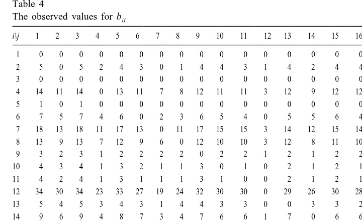
Table 4 shows the observed values b for the 20 letter series completion problems.ij First, we describe the analysis of the data with ITA. Only the relations #0 and #34
Table 3
Overview of the letter series completion problems used in the experiment. The third column shows the alphabetic relations holding between the subsequences of the series
Table 4
The observed values for bij
i\j 1 2 3 4 5 6 7 8 9 10 11 12 13 14 15 16 17 18 19 20
1 0 0 0 0 0 0 0 0 0 0 0 0 0 0 0 0 0 0 0 0
2 5 0 5 2 4 3 0 1 4 4 3 1 4 2 4 4 3 4 0 2
3 0 0 0 0 0 0 0 0 0 0 0 0 0 0 0 0 0 0 0 0
4 14 11 14 0 13 11 7 8 12 11 11 3 12 9 12 12 10 9 1 8
5 1 0 1 0 0 0 0 0 0 0 0 0 0 0 0 0 0 0 0 0
6 7 5 7 4 6 0 2 3 6 5 4 0 5 5 6 4 5 3 0 4
7 18 13 18 11 17 13 0 11 17 15 15 3 14 12 15 14 13 11 3 11
8 13 9 13 7 12 9 6 0 12 10 10 3 12 8 11 10 10 7 0 7
9 3 2 3 1 2 2 2 2 0 2 2 1 2 1 2 2 2 2 1 2
10 4 3 4 1 3 2 1 1 3 0 1 0 2 1 2 1 2 1 0 1
11 4 2 4 1 3 1 1 1 3 1 0 0 2 1 2 1 2 1 0 1
12 34 30 34 23 33 27 19 24 32 30 30 0 29 26 30 28 26 22 8 26
13 5 4 5 3 4 3 1 4 4 3 3 0 0 3 3 2 2 3 0 3
14 9 6 9 4 8 7 3 4 7 6 6 1 7 0 6 6 5 3 0 5
15 4 3 4 2 3 3 1 2 3 2 2 0 2 1 0 2 1 1 1 2
16 7 6 7 5 6 4 3 4 6 4 4 1 4 4 5 0 5 2 1 3
17 9 7 9 5 8 7 4 6 8 7 7 1 6 5 6 7 0 4 1 6
18 13 12 13 8 12 9 6 7 12 10 10 1 11 7 10 8 8 0 1 8
19 34 29 34 21 33 27 19 21 32 30 30 8 29 25 31 28 26 22 0 26
20 10 7 10 4 9 7 3 4 9 7 7 2 8 6 8 6 7 5 2 0
are transitive. The CA-value for #0 is higher than the CA-value for #34. The best surmise relation accordingly to ITA is therefore #0. This surmise relation is shown in Fig. 1 as a Hasse-Diagram.
The surmise relation #0 is organized in four layers. This surmise relation allows some conclusions concerning the difficulty of a letter series completion problem. The problems 1, 3, and 5 (layer 1 and 2) which contain an obvious identity relation (S) are the easiest, i.e. they are implied by all other problems. The problems 2, 4, 6, 8, 9, 10, 11, 13, 14, 15, 16, 17, 18, and 20 (layer 3) cannot be compared concerning their difficulty. The problems 7, 12, and 19 (layer 4) which contains a difficult alphabetic relation and have a high period seem to be the most complex problems. They imply some of the problems in layer 3.
This example shows that the handling of intransitivities in ITA is not satisfactory. If an intransitivity occurs the whole relation is dropped. This is problematic especially for
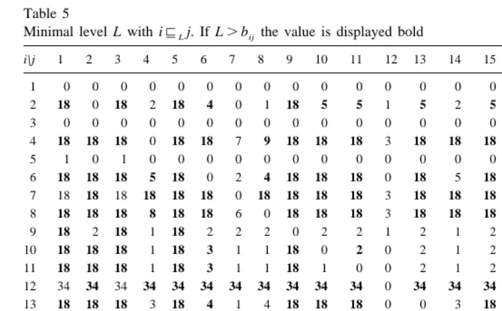
Table 5
big item sets, since the probability that at least one intransitivity occurs in #L increases with the size of the item set I.
*
We describe now the analysis of the dataset with ITA . Table 5 shows for each item pair the minimal level L for which i8 j is true. The values with b ±L are displayed
L ij
bold. Our inductive construction process allows us to construct 12 different surmise relations8L from the dataset R.
This example clearly shows the advantage of our inductive construction process. In ITA we have the choice between only two transitive relations (#0and#34). Using our inductive construction process we can select the best relation out of 12 transitive relations.
As an example for the inductive construction look at the items 6, 10 and 11. We have
b10,1151, b11,651 and b10,652. Thus, 10#111 and 11#16 but 10#⁄ 6. Therefore,1 #1
*
is intransitive. In ITA the pair (10, 11) is therefore not added in step 1 to the relation
level L9 is not displayed in the table, then 8L9 is identical to 8L for the highest displayed level L#L9.
The minimal diff-value is observed for L54. Therefore,84 is the optimal surmise relation. Note that 84 is more than double the size of 80 while the reproducibility coefficient decreases only a little.
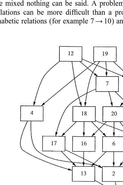
The relation 84 is shown in Fig. 2 as a Hasse-Diagram.
The relation84allows the following observations. If the alphabetic relations between the letters of the simple sequences are identical, the difficulty increases in general with
period length. See, for example, the implications 7→6, 12→8, and 19→4. For
problems with identical period length the difficulty increases in general with the complexity of the alphabetic relations used in the problem. See, for example, 8→2→1 or 12,19→7→3. Here S is less complex than N, N is less complex than P and D, while no such difference in difficulty between P and D could be observed. When both influences are mixed nothing can be said. A problem with high period length and easy alphabetic relations can be more difficult than a problem with low period length and complex alphabetic relations (for example 7→10) and vice versa (for example 4→13).
But in general the complexity of the alphabetic relations seems to be more important for problem difficulty than period length.
These results are consistent with formal theories of problem solving in the area of letter series completion problems (for example Kotovsky and Simon, 1973 or Klahr and Wallace, 1970). These theories assume that problem solvers first search for a possible relationship between two letters of the series. If such a relationship is detected, then it is used to uncover the period of the series. Finally, the information about the period is used to uncover the whole regularity in the series. Thus, problem complexity should mainly depend upon period length and the complexity of the alphabetic relations in the series.
6. Conclusions
*
The two simulation studies show that the ability of ITA and ITA to reconstruct the correct implications from data depends on the values fora,b, m and on the structure of
*
the underlying surmise relation. ITA performs better than ITA if the error probabilities
a, b are low and the underlying surmise relation contains only a few non-connected
*
item pairs. In the other cases ITA performs better than ITA.
Another observation is that the influence of the error probabilities a, b on the error
*
rate is much higher for ITA than for ITA . The effect of the structure of the underlying
*
surmise relation on the error rate is also much higher for ITA than for ITA . Thus, we
*
can conclude that ITA is much more stable against the influences of the error
probabilities and the structure of the underlying surmise relation than ITA.
If real sets of data patterns are analysed, then there is no information concerning the values of a and b available and the structure of the underlying surmise relation is of
*
course unknown. Since ITA is less influenced by these factors it seems to be preferable to ITA.
*
The simulation results show that ITA is highly reliable in reconstructing the correct implications. For a set of eight items as used in our simulations the algorithm must decide if j→i is true or not for 56 item pairs (since i→i is always correct). The number
of incorrect judgements is in general low. For example, for the surmise relation82and
a 5 b 50.07 in average two wrong judgements occur if 200 simulated data patterns are available.
*
In our practical application we used ITA to analyse a set of response patterns to letter series completion problems. The analysis leads to a surmise relation which reflects problem difficulty. A careful analysis of this surmise relation allows us to draw some conclusions on the connection between item structure and item difficulty. One possible
*
application of ITA is to analyse the influence of the internal structure of items on the property reflected by the surmise relation (for example item difficulty).
Another application is to use the constructed surmise relation as a basis for adaptive testing. Since i8ITA*j is interpreted as a logical implication it can be used to avoid
redundant questions. If a subject answers positive to item j a positive answer to all items
i with i8ITA*j can be inferred. These items must therefore not be presented to the
References
Bart, W.M., Krus, D.J., 1973. An ordering theoretic method to determine hierarchies among items. Educational and Psychological Measurement 33, 291–300.
Buggenhaut, J.v., Degreef, E., 1987. On dichotomization methods in boolean analysis of questionnaires. In: Roskam, E.E., Suck, R. (Eds.), Mathematical Psychology in Progress, Elsevier (North Holland). Doignon, J.P., Falmagne, J.C., 1985. Spaces for the assessment of knowledge. International Journal of
Man-Machine Studies 23, 175–196.
Duquenne, V., 1987. Conceptual implications between attributes and some representation properties for finite ¨
lattices. In: Ganter, B. et al. (Ed.), Beitrage zur Begriffsanalyse, Wissenschafts-Verlag, Mannheim, pp. 313–339.
Falmagne, J.-C., Doignon, J.-P., 1988. A Markovian procedure for assessing the state of a system. Journal of Mathematical Psychology 32, 232–258.
´
Flament, C., 1976. L’analyse booleenne de questionaire, Mouton, Paris.
Guttman, L., 1944. A basis for scaling qualitative data. American Sociological Review 9, 139–150. Held, T., Schrepp, M., Fries, S., 1995. Methoden zur Bestimmung von Wissensstrukturen-Eine
Vergleichs-¨
studie. Zeitschrift fur Experimentelle Psychologie XLII (2), S205–236.
Klahr, K., Wallace, J.G., 1970. The development of serial completion strategies: an information processing analysis. British Journal of Psychology 61, 243–257.
Kotovsky, K., Simon, H.A., 1973. Empirical tests of a theory of human acquisition of concepts for sequential patterns. Cognitive Psychology 4, 399–424.
Leeuwe, J.F.J.v., 1974. Item tree analysis. Nederlands Tijdschrift voor de Psychologie 29, 475–484. Schrepp, M., 1995. Modeling interindividual differences in solving letter series completion problems.
¨
Zeitschrift fur Psychologie 203, 173–188.